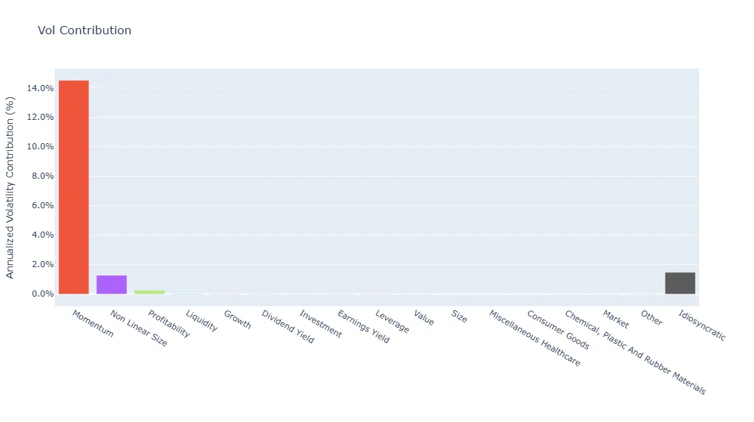
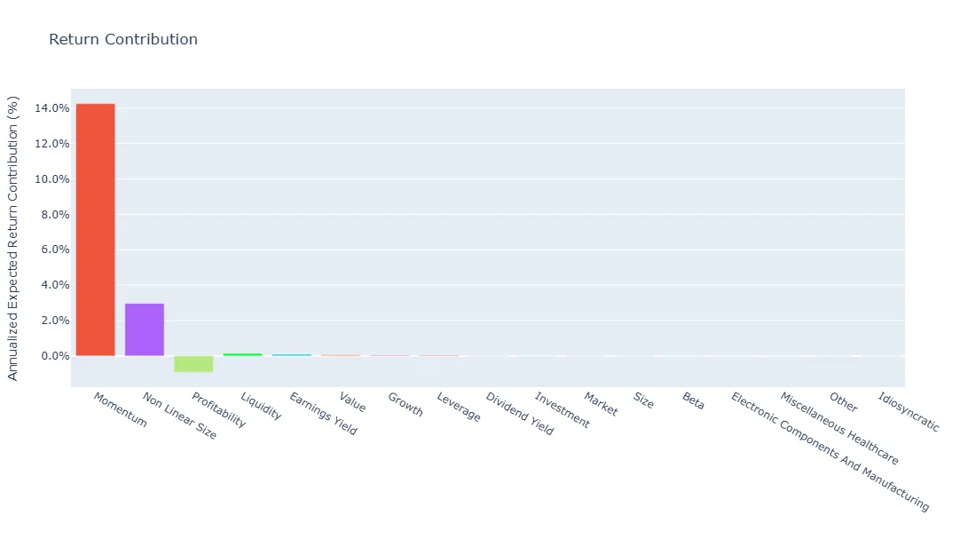
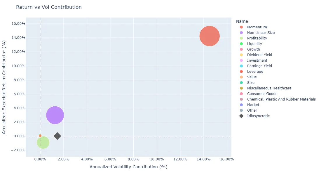
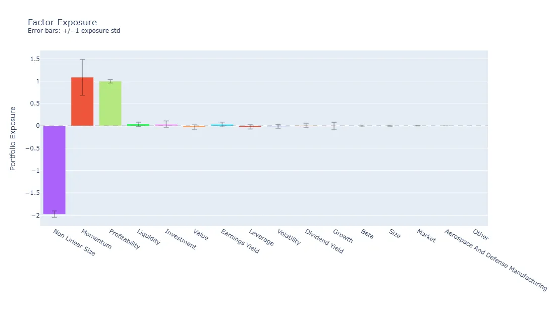
# Factor Models
This guide covers skfolio’s factor model implementations, their API and their
theoretical foundations. It focuses on the characteristics-based cross-sectional factor
model [`CharacteristicsFactorModel`](https://skfolio.org/generated/skfolio.prior.CharacteristicsFactorModel.html.md#skfolio.prior.CharacteristicsFactorModel). This model family has
become foundational in quantitative asset management, and implementing it correctly
requires addressing many practical challenges (e.g. point-in-time data, changing
universes, look-ahead bias, zero-sum constraints, alpha integration, diagnostics,
attribution and computational performance on large universes).
The results in this guide were obtained by fitting a 58-factor US equity model on
the FactSet
[Fundamentals Point-in-Time](https://www.factset.com/marketplace/catalog/product/factset-fundamentals-point-in-time),
[Estimates Point-in-Time Consensus](https://www.factset.com/marketplace/catalog/product/factset-estimates-point-in-time-consensus)
and [RBICS](https://www.factset.com/marketplace/catalog/product/factset-rbics-api)
datasets. The [Factor Models gallery](https://skfolio.org/auto_examples/factor_models/index.html.md#factor-models-examples) provides complete,
runnable tutorials using synthetic characteristics data, so users can explore the full API
while respecting data vendor licences.
For complementary references, see “The Elements of Quantitative Investing” by Giuseppe
Paleologo [1](#id6), “Active Portfolio Management” by Grinold and Kahn [2](#id7), and
“Portfolio Optimization: Theory and Application” by Daniel P. Palomar [3](#id8).
## Introduction
### Motivation and Use Cases
Directly estimating the covariance matrix of a large asset universe is impractical.
The sample covariance matrix of 5,000 assets has over 12 million free parameters and
requires more than 5,000 observations (~20 years of daily data) in order to reach full
rank. The resulting estimate is ill-conditioned, unstable and slow to react to change,
and an optimizer using that estimate will also tend to allocate toward the parts of the
covariance structure where estimation noise is largest.
A factor model addresses this problem by assuming that a small set of pervasive
factors (e.g. market, industries, countries, currencies, styles) drives the
co-movement of assets, and the remainder is asset-specific (i.e. idiosyncratic).
Estimation then reduces to a small factor covariance plus one idiosyncratic variance
per asset, requiring far fewer parameters and a much shorter history.
Factor models are used for:
* **Risk forecasting**: estimate a stable asset covariance matrix for large universes.
* **Risk decomposition**: express portfolio risk as systematic exposures plus
idiosyncratic risk, separating intended from unintended exposures.
* **Performance attribution**: explain realized returns factor by factor,
distinguishing systematic factor premia from asset-specific returns, and separating
skill from luck.
* **Portfolio construction**: supply expected returns, covariance, scenarios and
factor exposures to an optimizer, with exposures that can be monitored and
constrained.
* **Alpha research**: provide the ingredients of the alpha workflow, such as
idiosyncratic returns as a prediction target, idiosyncratic variances
for signal scaling, and factor exposures for neutralization.
* **Alpha decomposition**: split an alpha forecast into spanned alpha and orthogonal
alpha before optimization.
### Model Definition
A factor model decomposes asset returns into systematic and idiosyncratic
components:
$$
r_t = B \, f_t + \epsilon_t
$$
where:
* $B \in \mathbb{R}^{N \times K}$ is the factor exposure matrix, also called
the loading matrix: the sensitivity of each asset to each factor.
* $f_t \in \mathbb{R}^{K}$ is the vector of factor returns: the return per unit
of exposure at time $t$, common to all assets.
* $\epsilon_t \in \mathbb{R}^{N}$ is the vector of idiosyncratic returns: the
part of asset returns not explained by the factors.
The factor structure assumes that common co-movement is captured by the factors, and
that the remaining idiosyncratic covariance is diagonal or sparse. The asset
covariance matrix is:
$$
\Sigma = B \, F \, B^\top + D
$$
where $F \in \mathbb{R}^{K \times K}$ is the factor covariance matrix and
$D$ is the diagonal or sparse idiosyncratic covariance matrix.
The [Expected Returns](#factor-model-expected-returns) section explains how
[`CharacteristicsFactorModel`](https://skfolio.org/generated/skfolio.prior.CharacteristicsFactorModel.html.md#skfolio.prior.CharacteristicsFactorModel) estimates expected asset returns
from expected factor returns and an optional alpha forecast.
The rest of this guide covers the estimation of $B$, $f_t$, $F$,
and $D$, and their use in optimization and attribution.
### Types of Factor Models
Factor model families differ by what is observed before fitting: factor returns,
factor exposures, or neither.
**Time-series factor models** observe the factor returns and estimate asset exposures.
Factors are observable time series such as factor ETF returns, long-short factor portfolio
returns, or macroeconomic series (e.g. inflation, rates, GDP growth), hence the
alternative name “macroeconomic factor models”. Each asset’s exposures come from a
time-series regression of its returns on those factor series. They are interpretable,
straightforward to estimate, and they can work on small universes because each
asset is estimated independently. However, they require long return histories per asset,
exposures react slowly to asset-level change because they only update through the
regression window, and the risk of misspecification is higher. When factors are
tradable, their return history can be used to estimate factor premia. For
non-tradable variables, factor premia are estimated with a second-pass
cross-sectional procedure such as Fama-MacBeth on a sufficiently broad universe.
Implemented in [`TimeSeriesFactorModel`](https://skfolio.org/generated/skfolio.prior.TimeSeriesFactorModel.html.md#skfolio.prior.TimeSeriesFactorModel).
**Characteristics-based factor models**, also called “fundamental factor models”, observe
exposures and estimate factor returns. Exposures are built from point-in-time
asset characteristics (e.g. industry classification, country, market capitalization,
book equity, sales, operating cash flow, analyst estimates), and factor returns are derived
from one cross-sectional regression of asset returns on exposures at each date.
Exposures react immediately to asset-level change, new assets need no return history to
receive exposures, and factors can be neutralized against each other to produce pure
factor definitions. The challenges of this model are the complexity of the estimation
procedure and the heavier data requirement, both of which are covered in this guide.
Implemented in [`CharacteristicsFactorModel`](https://skfolio.org/generated/skfolio.prior.CharacteristicsFactorModel.html.md#skfolio.prior.CharacteristicsFactorModel).
#### NOTE
The Fama-French procedure also starts from characteristics, but follows a different
construction. It uses characteristics to sort assets into quantile long-short
portfolios whose returns define the factors. It is primarily a factor-pricing
framework for explaining the cross-section of expected returns, as opposed to a full
risk model. To use those factor returns as a risk model for arbitrary assets, exposures
must be estimated by time-series regression, inheriting the drawbacks of
time-series factor models.
Moreover, quantile portfolios are not pure factors in the characteristics
risk-model sense. A value portfolio, for example, can also carry industry, size,
profitability, investment or momentum tilts because the sorting procedure only
controls the characteristics used to build the portfolio. Intersection procedures
reduce this contamination by sorting on several characteristics at the same time,
but they do not scale to a large number of factors.
**Statistical factor models** observe neither factor returns nor exposures and instead
extract both from asset returns using methods such as PCA. They are adaptive and need
returns only, but factors have no economic identity and may drift across regimes.
Currently not implemented in skfolio.
### Historical Background
Characteristics factor models originate with Barr Rosenberg, whose 1974 work on
extra-market components of covariance [4](#id9) showed that asset characteristics predict
return covariation, and that a small set of common factors explains most
cross-sectional variation while the residual is asset-specific. Rosenberg founded
Barra (now part of MSCI) to commercialize the approach, and the first US equity model
(USE1) was released in 1975. Specialist competitors followed, including Northfield
(1985), Axioma (1998) and Wolfe Research (2008). Data vendors later entered the market
by adding proprietary factor models to their data and analytics platforms, including
Bloomberg, FactSet, S&P Global and Morningstar. Factor risk models have since become
standard infrastructure across quantitative hedge funds, asset managers and banks.
These models were initially built for risk estimation, but practitioners observed
that some risk factors (e.g. value, momentum) also earn persistent premia. Modern
implementations therefore estimate expected factor returns alongside factor
covariances, enabling deliberate tilts toward specific factors in optimization, the
foundation of what became known as “smart beta”.
Today, commercial factor risk models are often distributed as model catalogues, usually segmented by
region and horizon. skfolio now provides a toolkit for building and customizing factor models directly
from user-defined data, rather than selecting a single predefined model from a catalogue. This enables a
continuum of specifications, recognizing the view that there is no “one size fits all” factor model.
### Alternatives to a Single Centralized Factor Model
A factor model is an estimate. Its exposures, factor covariance and
idiosyncratic variances carry estimation error, and its specification is never
complete, as no factor set captures all common co-movement.
The traditional commercial offering can lead to a single house risk model
being shared by all strategies and risk management teams. skfolio supports
this approach but also allows for an alternative approach where the factor model is
itself an estimator parameter, such that each strategy can embed its own specific
factor model. The strategy and its factor model then form a single meta-model that is fitted,
evaluated and tuned jointly.
Multiple factor models allow portfolio construction and risk monitoring to use different model
specifications. A portfolio may be constructed with a factor model tailored to its universe,
horizon and alpha process, while risk management evaluates exposures and covariance with a
broader firm-wide model. At the book level, using different factor models across portfolios
and strategies introduces model diversification. Estimation error and specification error are
then distributed across model specifications rather than concentrated in a single shared model.
## Model Overview
### Estimation Pipeline
[`CharacteristicsFactorModel`](https://skfolio.org/generated/skfolio.prior.CharacteristicsFactorModel.html.md#skfolio.prior.CharacteristicsFactorModel) is a meta-estimator following
scikit-learn conventions. It composes sub-estimators, descriptors, factor exposure
estimators, a cross-sectional regressor, prior estimators for factor and idiosyncratic
risk and an optional alpha estimator, each of which can be replaced, tuned and
customized independently. The input is a point-in-time
[`AssetPanel`](https://skfolio.org/generated/skfolio.containers.AssetPanel.html.md#skfolio.containers.AssetPanel) of asset characteristics and the output is a
[`ReturnDistribution`](https://skfolio.org/generated/skfolio.prior.ReturnDistribution.html.md#skfolio.prior.ReturnDistribution) consumed by all skfolio optimizations,
together with a [`FactorModel`](https://skfolio.org/generated/skfolio.prior.FactorModel.html.md#skfolio.prior.FactorModel) container holding the full
decomposition and diagnostics.
The model is fitted as follows:
1. Start from point-in-time asset characteristics stored as panel fields (e.g.
`returns`, `market_cap`, `book_equity`, `industry`).
2. Compute descriptor values from these fields, or pass through existing fields
unchanged, using descriptor estimators.
3. Build factor exposures. Style factors are typically formed by combining one or
more descriptors and applying cross-sectional transformations (e.g. winsorization,
z-scoring). Categorical factors (e.g. industry, country, currency) are represented
by one-hot exposures.
4. Orthogonalize selected exposures against other factors or families when
`neutralize_against` is provided.
5. Reparameterize constrained families when `constrained_families` is provided. This
enforces the benchmark-weighted zero-sum constraint on factor returns within each
constrained family and produces a full-rank basis for factor-level estimators.
6. Estimate realized factor returns with
`cs_regressor` on the estimation universe defined by the panel’s
`estimation_mask`. By default, regression weights are based on market
capitalization through `regression_mcap_power`. When
`inv_idio_variance_weight_shrinkage > 0`, a two-pass procedure blends those weights
with inverse-idiosyncratic-variance weights estimated from first-pass residuals.
7. Estimate the factor return distribution with `factor_prior_estimator`, including
expected factor returns (factor premia), factor covariance and factor return
scenarios. This step can introduce factor covariance shrinkage, short-term
volatility updating or Newey-West HAC correction.
8. Estimate idiosyncratic variances with `idio_variance_estimator`, then form the
idiosyncratic covariance as a diagonal matrix or, when `idio_corr_threshold > 0`,
as a sparse covariance using correlation thresholding.
9. If provided, fit `alpha_estimator` to produce an alpha forecast. Decompose it into
spanned alpha and orthogonal alpha, blend factor-implied asset expected returns with
the spanned alpha using `spanned_alpha_shrinkage`, shrink the orthogonal alpha
with `orthogonal_alpha_confidence` and assemble the final $\mu$,
$\Sigma$ and asset return scenarios on the investment universe.
Each step is detailed in the following sections.
### Code Example
The model below is used throughout this guide. It is a medium-horizon US equity model
with 58 factors: 1 global factor, 44 industry factors and 13 style factors built from
29 descriptors. It uses within-industry scoring, neutralization, a zero-sum constraint
on the industry family, regression weights that blend market-capitalization weights
with inverse-idiosyncratic-variance weights and a regime-adjusted factor covariance
estimator. The model was fitted on the FactSet point-in-time datasets of 2,000 US
equities with daily data from 2013 to 2026. The parametrization is intentionally
simple and has not been fine-tuned. This simplified model is used as the standard
example for presenting the API. See [Hyperparameter Tuning](#factor-model-hyper-parameter-tuning) for guidance on tuning the model to your data
and goals.
```python
from skfolio.descriptor import (
AssetsGrowthRate,
AssetTurnover,
BookLeverage,
BookToPrice,
CapexToAssetsChangeInIntensity,
CashFlowToAssets,
CashFlowToPrice,
DebtToAssets,
DividendToPrice,
EarningsChangeToPrice,
EarningsToPrice,
EbitdaToEnterpriseValue,
EWAmihudIlliquidity,
EWMarketBeta,
EWMomentum,
EWResidualVolatility,
EWShareTurnover,
EWVolatility,
ForwardEarningsToPrice,
GrossMargin,
GrossProfitability,
IssuanceGrowthRate,
LogMarketCap,
MarketLeverage,
ReturnOnAssets,
ReturnOnEquity,
SalesGrowthRate,
SalesToPrice,
ShareholderYield,
)
from skfolio.factor_exposure import (
DerivedFactor,
FixedWeightedFactor,
GlobalFactor,
OneHotCategoricalFactors,
)
from skfolio.moments import EWMu, RegimeAdjustedEWCovariance
from skfolio.prior import CharacteristicsFactorModel, EmpiricalPrior
month = 21
quarter = 3 * month
half_year = 6 * month
year = 12 * month
# Global factor
global_factor = GlobalFactor(family="market")
# Industry factors
industry_factors = OneHotCategoricalFactors(category="industry", family="industry")
# Style factors
beta_factor = FixedWeightedFactor(
descriptors=[("market_beta", EWMarketBeta(half_life=year))],
transform_by_group="industry",
)
momentum_factor = FixedWeightedFactor(
descriptors=[("momentum", EWMomentum(half_life=half_year, skip=month))],
transform_by_group="industry",
)
size_factor = FixedWeightedFactor(
descriptors=[("log_mcap", LogMarketCap())], transform_by_group="industry"
)
non_linear_size_factor = DerivedFactor(
source="size", func=lambda x: x**3, transform_by_group="industry"
)
value_factor = FixedWeightedFactor(
descriptors=[
("book_to_price", BookToPrice()),
("sales_to_price", SalesToPrice()),
("cash_flow_to_price", CashFlowToPrice()),
],
weights=[0.8, 0.1, 0.1],
transform_by_group="industry",
)
earnings_yield_factor = FixedWeightedFactor(
descriptors=[
("fwd_earnings_to_price", ForwardEarningsToPrice()),
("earnings_to_price", EarningsToPrice()),
("enterprise_multiple", EbitdaToEnterpriseValue()),
],
transform_by_group="industry",
)
growth_factor = FixedWeightedFactor(
descriptors=[
("earnings_change_to_price", EarningsChangeToPrice(lag=year)),
("sales_growth", SalesGrowthRate(lag=year)),
],
transform_by_group="industry",
)
profitability_factor = FixedWeightedFactor(
descriptors=[
("asset_turnover", AssetTurnover()),
("gross_profitability", GrossProfitability()),
("gross_margin", GrossMargin()),
("return_on_assets", ReturnOnAssets()),
("return_on_equity", ReturnOnEquity()),
("cash_flow_to_assets", CashFlowToAssets()),
],
transform_by_group="industry",
)
investment_factor = FixedWeightedFactor(
descriptors=[
("asset_growth", AssetsGrowthRate(lag=year)),
("issuance_growth", IssuanceGrowthRate(lag=year)),
("capex_growth", CapexToAssetsChangeInIntensity(lag=year)),
],
transform_by_group="industry",
)
dividend_yield_factor = FixedWeightedFactor(
descriptors=[
("dividend_to_price", DividendToPrice()),
("shareholder_yield", ShareholderYield()),
],
weights=[0.7, 0.3],
transform_by_group="industry",
)
leverage_factor = FixedWeightedFactor(
descriptors=[
("market_leverage", MarketLeverage()),
("debt_to_assets", DebtToAssets()),
("book_leverage", BookLeverage()),
],
transform_by_group="industry",
)
liquidity_factor = FixedWeightedFactor(
descriptors=[
("share_turnover", EWShareTurnover(half_life=quarter)),
("amihud_illiquidity", EWAmihudIlliquidity()),
],
transform_by_group="industry",
)
volatility_factor = FixedWeightedFactor(
descriptors=[
("vol", EWVolatility(half_life=quarter)),
(
"residual_vol",
EWResidualVolatility(half_life=quarter, beta_half_life=quarter),
),
],
transform_by_group="industry",
)
# Characteristics Factor Model
model = CharacteristicsFactorModel(
factors=[
("market", global_factor),
("industry", industry_factors),
("beta", beta_factor),
("momentum", momentum_factor),
("size", size_factor),
("non_linear_size", non_linear_size_factor),
("value", value_factor),
("earnings_yield", earnings_yield_factor),
("growth", growth_factor),
("profitability", profitability_factor),
("investment", investment_factor),
("dividend_yield", dividend_yield_factor),
("leverage", leverage_factor),
("liquidity", liquidity_factor),
("volatility", volatility_factor),
],
neutralize_against={
"non_linear_size": ["size"],
"volatility": ["beta"],
},
constrained_families=[("industry", None)],
exposure_lag=1,
inv_idio_variance_weight_shrinkage=0.5,
factor_prior_estimator=EmpiricalPrior(
covariance_estimator=RegimeAdjustedEWCovariance(
half_life=half_year, corr_half_life=year, regime_half_life=month
),
mu_estimator=EWMu(half_life=year),
),
n_jobs=-1,
)
```
The model is fitted on a point-in-time [`AssetPanel`](https://skfolio.org/generated/skfolio.containers.AssetPanel.html.md#skfolio.containers.AssetPanel) whose
construction is covered in the [Input Data](#factor-model-input-data) section:
```python
model.fit(characteristics=characteristics)
```
For incremental updates on new observations, use `partial_fit`, covered in the
[Online Learning](#factor-model-online-learning) section:
```python
model.partial_fit(characteristics=new_characteristics)
```
After fitting, the model exposes two main attributes.
`return_distribution_` is the [`ReturnDistribution`](https://skfolio.org/generated/skfolio.prior.ReturnDistribution.html.md#skfolio.prior.ReturnDistribution) consumed by
skfolio optimizations. It contains the expected asset returns `mu`, the asset
covariance matrix `covariance` and the asset return scenarios `returns`, all on the
investment universe. Assets that are not investable at the current point in time
(e.g. delisted, not yet listed, or still in [warmup](#factor-model-warmup))
are represented with NaN.
`factor_model_` is the [`FactorModel`](https://skfolio.org/generated/skfolio.prior.FactorModel.html.md#skfolio.prior.FactorModel) container holding the full
decomposition: factor exposures, loading matrix, factor returns, expected factor
returns and factor covariance, idiosyncratic returns, variances and covariance,
regression and benchmark weights. It provides DataFrame accessors (`factor_returns_df`,
`idio_returns_df`, `exposures_df`), slicing (`select_assets`, `select_observations`),
a `summary` method and the diagnostic statistics and plots covered in the
[Diagnostics](#factor-model-diagnostics) section.
```python
distribution = model.return_distribution_
distribution.mu # expected returns, shape (n_assets,)
distribution.covariance # asset covariance, shape (n_assets, n_assets)
distribution.returns # return scenarios, shape (n_observations, n_assets)
factor_model = model.factor_model_
factor_model.summary()
factor_model.factor_returns_df()
```
The fitted sub-estimators are also available with the usual scikit-learn trailing
underscore convention: `cs_regressor_`, `factor_prior_estimator_`,
`idio_variance_estimator_`, `idio_corr_estimator_` and `alpha_estimator_`.
The `X` argument of `fit` is optional. When provided, `X` selects the investment
universe: its columns define the assets returned in `return_distribution_` and
`factor_model_`. Factor estimation still uses the `returns` field of
`characteristics`, which can cover a broader point-in-time universe. This keeps the
estimator compatible with skfolio pipelines, cross-validation, prediction and scoring.
When `X` is `None`, the investment universe equals the coverage universe.
## Input Data
The model consumes a point-in-time [`AssetPanel`](https://skfolio.org/generated/skfolio.containers.AssetPanel.html.md#skfolio.containers.AssetPanel) of asset
characteristics. The panel must include a `returns` field and, when market-cap
weighting is used, a `market_cap` field. The remaining fields depend on the chosen
descriptors and alpha estimators. The [example](#factor-model-code-example)
model uses market data (e.g.
`adj_close`, `adj_volume`, `adj_shares_outstanding`), fundamentals (e.g.
`book_equity`, `sales_ttm`, `total_assets`, `operating_cash_flow_ttm`), analyst
estimates (e.g. `eps_ntm`, `dps_ntm`) and a categorical `industry` field.
### AssetPanel Container
A factor model pipeline applies many cross-sectional and time-series transformations
to the same date-by-asset data. With general-purpose containers (e.g. DataFrames, xarray),
each step must re-align indexes, group by date or pivot before computing. This adds
overhead and increases the risk of indexing errors, either on the time index, which
can introduce look-ahead bias, or on the asset index. To address this, skfolio provides
[`AssetPanel`](https://skfolio.org/generated/skfolio.containers.AssetPanel.html.md#skfolio.containers.AssetPanel), a dedicated container for aligned
cross-sectional asset data. An [`AssetPanel`](https://skfolio.org/generated/skfolio.containers.AssetPanel.html.md#skfolio.containers.AssetPanel) validates
alignment once so that estimators operate on already-aligned numeric arrays and stores
universe masks explicitly, which is needed for point-in-time estimation on changing
universes (e.g. listing, delisting, inclusion/exclusion rules).
The rationale behind the container, the wide-format convention and the NaN-handling
conventions are covered in [Asset Data Representation](https://skfolio.org/user_guide/data_representation.html.md#asset-data-representation).
Every field shares the same two axes with shape `(n_observations, n_assets)`. Three
kinds of fields are supported:
* 2D numeric fields (e.g. `returns`, `market_cap`)
* 2D categorical fields (e.g. `industry`, `country`), stored as integer codes with
their category labels
* 3D numeric fields (e.g. factor exposures), with labeled third axis
The panel also carries two boolean masks aligned with the data, `active_mask` and
`estimation_mask`, described in [Coverage, Estimation and Investment
Universes](#factor-model-universes).
This layout has additional practical benefits:
* The container is scikit-learn compatible: `len(panel)` returns the number of
observations and `panel[start:stop]` returns a zero-copy view, so the panel can be
passed directly to cross-validation and hyper-parameter tuning utilities, and
walk-forward folds reuse the same field arrays instead of copying them.
* With thread-based parallelism, workers read the same panel in memory instead of
receiving separate process copies, which is significant for large panels.
* Panels are saved as `.npy` files and support memory-mapped loading for fast
startup on large datasets.
```python
import numpy as np
from skfolio.containers import AssetPanel
from skfolio.datasets import make_synthetic_characteristics
# Build a panel from aligned date-by-asset arrays.
panel = AssetPanel(
fields={
"returns": returns, # ndarray (n_observations, n_assets)
"market_cap": market_cap, # ndarray (n_observations, n_assets)
},
observations=dates,
asset_names=assets,
active_mask=active_mask,
estimation_mask=estimation_mask,
)
panel.add_categorical_field(
name="industry",
values=industry_codes, # integer codes (n_observations, n_assets)
levels=["energy", "bank", "technology"],
)
# Inspect dimensions, fields, missing values and mask coverage.
panel.info()
# Save and reload a panel.
panel.save("path/to/saved_panel")
saved_panel = AssetPanel.load("path/to/saved_panel")
# Generate a synthetic panel for examples and tests.
characteristics = make_synthetic_characteristics()
```
### Coverage, Estimation and Investment Universes
A factor model distinguishes three universes:
* The **coverage universe** is the full set of assets stored in the
[`AssetPanel`](https://skfolio.org/generated/skfolio.containers.AssetPanel.html.md#skfolio.containers.AssetPanel). It contains the estimation universe and
the investment universe.
* The **estimation universe**, defined by the panel’s `estimation_mask`, is the
subset of observation-asset pairs used to fit cross-sectional statistics,
factor-return regressions, benchmark and regression weights, alpha estimators and
regime statistics. Pairs outside it still receive transformed values, exposures and
forecasts, but do not contribute to those fitted statistics.
* The **investment universe** is the set of assets selected for portfolio
optimization. It is returned in `return_distribution_` and
`factor_model_`. When `X` is provided to `fit`, its columns select this universe.
When `X` is `None`, the investment universe equals the coverage universe. This lets
the model estimate factors on a broader cross-section, then return outputs only for
the assets used downstream.
Membership within the coverage universe varies through time and is tracked by the
panel’s `active_mask`. `False` marks an asset outside the universe at that date
(e.g. pre-listing, post-delisting), while `True` with a NaN value marks missing data
for an active asset (e.g. holiday, missing quote). The `estimation_mask` is enforced
as a subset of `active_mask`.
The estimation universe must be broad enough to represent the investment opportunity
set, liquid enough to avoid spurious return relationships and stable enough for factor
exposures to behave consistently through time. For a US equity model, a typical
estimation universe is 1,000 to 3,000 names. It should also be large enough relative to the
factor set. The number of estimation assets $N$ should be well above the number of
factors $K$ for a stable cross-sectional regression, and best practice is to have
at least 20 estimation assets per industry (e.g. 50 industries require at least
1,000 assets in a well-balanced universe, and more if some industries are sparsely
represented).
The effective size of the estimation universe also depends on the regression weights.
The default square-root market-capitalization weights are commonly used as a proxy for
inverse idiosyncratic variance. Under this default weighting, the contribution of
small stocks decreases rapidly: relative to the full universe of investable US
equities, the largest 2,000 stocks represent about 99% of total market capitalization
and would carry roughly 90% of the total regression weight. Extending the universe
beyond this point can still be useful when the additional names improve estimation
of small-cap-sensitive factors or increase coverage of sparsely represented industries.
Otherwise, extending the estimation universe further mostly adds memory and compute cost
and may add noise from illiquid securities (e.g. stale prices, zero-return days,
bid-ask bounce, missing fundamentals).
### Point-in-Time Data
AssetPanel characteristics should be built from point-in-time (PIT) datasets. For
fundamentals, this means respecting reporting lags and using the figures as reported
at the time, before later restatements. Data vendors offer point-in-time datasets for
this purpose, and the example in this guide is constructed using FactSet point-in-time datasets.
When actual availability dates are not available, a common fallback is to apply a
conservative lag from the fiscal period end, such as 90 days, before making the value
available to the model.
Let’s suppose ABC’s fiscal Q2 ends on 2024-06-30, Q2 sales are reported as 100m
on 2024-08-05, and later restated to 96m on 2024-11-12. If the latest available
Q1 sales value is 90m before the Q2 report, a daily `AssetPanel` stores:
| Observation date | Sales value in the PIT panel | Source available on that date |
|--------------------|--------------------------------|---------------------------------|
| 2024-08-01 | 90m | Latest available Q1 value |
| 2024-08-02 | 90m | Latest available Q1 value |
| 2024-08-05 | 100m | 2024 Q2 report |
| 2024-08-06 | 100m | Latest available Q2 value |
| 2024-11-12 | 96m | 2024 Q2 restatement |
Universe membership must also be point-in-time. The universe is formed by applying
eligibility rules at each observation date, using fields known on that date such as
listing status, market capitalization, liquidity, sector, country, exchange and
security type. Fitting history on the current constituent list introduces survivorship
bias as assets that were delisted, acquired or defaulted disappear from the sample,
biasing both estimates. See
[data representation](https://skfolio.org/user_guide/data_representation.html.md#asset-data-representation) for missing data, changing
universes and `active_mask`.
### Time Alignment and Look-Ahead Bias
To avoid look-ahead bias from inconsistent time indexing and manual lagging across
characteristic fields, exposures and returns, skfolio uses a single as-of
time-indexing convention across all estimators, so data is aligned once and lags
enter as model parameters.
Under this convention, all time-varying inputs at observation $t$ reflect
information available up to and including the end of period $t$. Point-in-time
fields and derived values (e.g. prices, fundamentals, industry labels and factor
exposures) store the latest available value for observation $t$. Returns
stored at observation $t$ cover the period ending at $t$, namely
$(t-1, t]$.
Factor-return regressions estimate the factor returns realized over
$(t-1, t]$. The exposure matrix must therefore describe the assets before that
return interval begins, at $t-1$. `exposure_lag` selects that
exposure date and defaults to 1:
$$
R(t) = B(t - \ell)\,f(t) + \epsilon(t)
$$
where $\ell$ is `exposure_lag`. With the default $\ell = 1$, returns over
$(t-1, t]$ are regressed on exposures measured at $t-1$.
At each observation, this regression estimates realized factor returns and
idiosyncratic returns $\epsilon(t)$. Expected asset returns are subsequently
constructed from expected factor returns and, when configured, an alpha forecast.
The same alignment applies to regression weights. Market capitalization weights are
lagged by `exposure_lag`, and inverse-idiosyncratic-variance weights at date
$t$ are estimated from residuals up to $t-1$. Both are detailed in the
[Regression Weights](#factor-model-regression-weights) section.
Stored outputs follow the as-of time-indexing convention. `factor_model_.exposures` at $t$
stores the exposures measured at $t$, and the covariance forecast pairs the
factor covariance with the latest exposures $B(T)$. The lag is applied
internally when estimating realized factor returns and regression-based statistics.
### Split, Dividend and Excess Return Conventions
The `returns` field should contain total returns, computed from split and dividend
adjusted prices. It is the dependent variable of the cross-sectional regression and
the input to all return-based descriptors (beta, volatility, momentum, reversal).
Other market data used by descriptors, such as prices, trading volumes and shares
outstanding, should be split adjusted but not dividend adjusted. These enter
descriptors as price and quantity levels, for example as the denominator of a
valuation ratio or in turnover and liquidity measures, where reinvested dividends
would distort the level. The corresponding fields are detailed in the
[Descriptors](#factor-model-descriptor-input-fields) section. The `market_cap`
field should contain the market value of common equity at each date.
In a single-currency model, raw and excess returns give nearly identical regression
results, as subtracting a common risk-free rate shifts the cross-section by a constant
that the global factor absorbs. Excess returns remain preferable because
some descriptors estimate time-series regressions (e.g.
[`EWMarketBeta`](https://skfolio.org/generated/skfolio.descriptor.EWMarketBeta.html.md#skfolio.descriptor.EWMarketBeta),
[`EWResidualVolatility`](https://skfolio.org/generated/skfolio.descriptor.EWResidualVolatility.html.md#skfolio.descriptor.EWResidualVolatility)) whose time-series intercept should
capture residual return without absorbing the risk-free rate. In a multi-currency model,
`returns` should contain local excess returns, and currency excess returns are
supplied through the `currency_excess_returns` argument. See the [Currency
Factors](#factor-model-currency-factors) section.
## Factor Exposures
Factor exposure estimators transform an [`AssetPanel`](https://skfolio.org/generated/skfolio.containers.AssetPanel.html.md#skfolio.containers.AssetPanel) into
factor exposure arrays. Some estimators compute
exposures without descriptors, such as the global market factor or one-hot industry
factors. Others compute one or more descriptors and transform them into standardized
style exposures.
skfolio provides four factor exposure estimators:
* [`GlobalFactor`](https://skfolio.org/generated/skfolio.factor_exposure.GlobalFactor.html.md#skfolio.factor_exposure.GlobalFactor) creates one common factor by
assigning every asset an exposure of 1.0. In the cross-sectional regression,
this factor acts as the cross-sectional regression intercept or broad market
factor. With the
benchmark-weighted centering and zero-sum constraints described in
[Global Factor and Benchmark Portfolio](#factor-model-global-factor), its
estimated factor return captures the benchmark portfolio return.
* [`OneHotCategoricalFactors`](https://skfolio.org/generated/skfolio.factor_exposure.OneHotCategoricalFactors.html.md#skfolio.factor_exposure.OneHotCategoricalFactors) turns a categorical
field into binary membership factors, one factor per category level. An asset has
exposure 1.0 to the factor matching its category and 0.0 to the other
category factors.
* [`FixedWeightedFactor`](https://skfolio.org/generated/skfolio.factor_exposure.FixedWeightedFactor.html.md#skfolio.factor_exposure.FixedWeightedFactor) builds a factor from one or
more descriptors. Each descriptor is computed, passed through the outlier and
scoring transforms, and converted into a cross-sectional score. The descriptor
scores are then aggregated with the fixed descriptor weights. For each
asset-observation pair, non-finite scores are ignored and the weighted average is
divided by the weight assigned to the remaining finite scores, so an asset missing
a descriptor (e.g. gross margin for financial firms, which do not report cost of
goods sold) can still receive a composite score from its valid descriptors. The
`min_coverage` parameter sets the minimum fraction of descriptor weight that must
be finite and when below this threshold, the composite is NaN. When multiple descriptors
are combined and scoring is enabled, the composite is scored again cross-sectionally
so partial-coverage composites remain on a comparable scale.
* [`DerivedFactor`](https://skfolio.org/generated/skfolio.factor_exposure.DerivedFactor.html.md#skfolio.factor_exposure.DerivedFactor) applies a function to another
factor’s exposure, then optionally applies outlier and scoring transforms. In
the [example](#factor-model-code-example), it builds the non-linear size
factor from the size exposure (`func=lambda x: x**3`). Dependencies between
factors are resolved automatically through topological sorting.
Custom exposure estimators are created by subclassing
[`BaseFactorExposure`](https://skfolio.org/generated/skfolio.factor_exposure.BaseFactorExposure.html.md#skfolio.factor_exposure.BaseFactorExposure).
Every factor exposure estimator carries a `family` attribute (e.g. `"market"`,
`"style"`, `"industry"`, `"country"`, `"currency"`). Families group related factors and
are used in neutralization, zero-sum constraints, attribution and reporting.
### Descriptors
A descriptor is a transformer that reads one or more
[`AssetPanel`](https://skfolio.org/generated/skfolio.containers.AssetPanel.html.md#skfolio.containers.AssetPanel) fields and returns a value array of shape
`(n_observations, n_assets)`. Descriptors follow the as-of time-indexing convention: values at
observation $t$ use information available up to and including the end of period
$t$.
skfolio provides descriptors covering the standard factor literature:
| Category | Descriptors |
|------------------|---------------------------------------------------------------------------------------------------------------------------------------------------------------------------------------------------------------------------------------------------------------------------------------------------------------------------------------------------------------------------------------------------------------------------------------------------------------------------------------------------------------------------------------------------------------------------------------------------------------------------------------------------------------------------------------------------------------------------------------------------------------------------------------------------------------------------------------------------------------------------------------------------------------------|
| Value | * [`BookToPrice`](https://skfolio.org/generated/skfolio.descriptor.BookToPrice.html.md#skfolio.descriptor.BookToPrice) * [`CashFlowToPrice`](https://skfolio.org/generated/skfolio.descriptor.CashFlowToPrice.html.md#skfolio.descriptor.CashFlowToPrice) * [`SalesToPrice`](https://skfolio.org/generated/skfolio.descriptor.SalesToPrice.html.md#skfolio.descriptor.SalesToPrice) |
| Earnings yield | * [`EarningsToPrice`](https://skfolio.org/generated/skfolio.descriptor.EarningsToPrice.html.md#skfolio.descriptor.EarningsToPrice) * [`ForwardEarningsToPrice`](https://skfolio.org/generated/skfolio.descriptor.ForwardEarningsToPrice.html.md#skfolio.descriptor.ForwardEarningsToPrice) * [`EbitdaToEnterpriseValue`](https://skfolio.org/generated/skfolio.descriptor.EbitdaToEnterpriseValue.html.md#skfolio.descriptor.EbitdaToEnterpriseValue) |
| Growth | * [`AssetsGrowthRate`](https://skfolio.org/generated/skfolio.descriptor.AssetsGrowthRate.html.md#skfolio.descriptor.AssetsGrowthRate) * [`SalesGrowthRate`](https://skfolio.org/generated/skfolio.descriptor.SalesGrowthRate.html.md#skfolio.descriptor.SalesGrowthRate) * [`EarningsChangeToPrice`](https://skfolio.org/generated/skfolio.descriptor.EarningsChangeToPrice.html.md#skfolio.descriptor.EarningsChangeToPrice) * [`IssuanceGrowthRate`](https://skfolio.org/generated/skfolio.descriptor.IssuanceGrowthRate.html.md#skfolio.descriptor.IssuanceGrowthRate) * [`CapexToAssetsChangeInIntensity`](https://skfolio.org/generated/skfolio.descriptor.CapexToAssetsChangeInIntensity.html.md#skfolio.descriptor.CapexToAssetsChangeInIntensity) * [`GrowthRate`](https://skfolio.org/generated/skfolio.descriptor.GrowthRate.html.md#skfolio.descriptor.GrowthRate) * [`ChangeToScale`](https://skfolio.org/generated/skfolio.descriptor.ChangeToScale.html.md#skfolio.descriptor.ChangeToScale) * [`ChangeInIntensity`](https://skfolio.org/generated/skfolio.descriptor.ChangeInIntensity.html.md#skfolio.descriptor.ChangeInIntensity) |
| Profitability | * [`GrossProfitability`](https://skfolio.org/generated/skfolio.descriptor.GrossProfitability.html.md#skfolio.descriptor.GrossProfitability) * [`GrossMargin`](https://skfolio.org/generated/skfolio.descriptor.GrossMargin.html.md#skfolio.descriptor.GrossMargin) * [`ReturnOnAssets`](https://skfolio.org/generated/skfolio.descriptor.ReturnOnAssets.html.md#skfolio.descriptor.ReturnOnAssets) * [`ReturnOnEquity`](https://skfolio.org/generated/skfolio.descriptor.ReturnOnEquity.html.md#skfolio.descriptor.ReturnOnEquity) * [`AssetTurnover`](https://skfolio.org/generated/skfolio.descriptor.AssetTurnover.html.md#skfolio.descriptor.AssetTurnover) * [`CashFlowToAssets`](https://skfolio.org/generated/skfolio.descriptor.CashFlowToAssets.html.md#skfolio.descriptor.CashFlowToAssets) * [`SalesToEnterpriseValue`](https://skfolio.org/generated/skfolio.descriptor.SalesToEnterpriseValue.html.md#skfolio.descriptor.SalesToEnterpriseValue) |
| Earnings quality | * [`AccrualsCashFlow`](https://skfolio.org/generated/skfolio.descriptor.AccrualsCashFlow.html.md#skfolio.descriptor.AccrualsCashFlow) * [`AnalystDispersionToPrice`](https://skfolio.org/generated/skfolio.descriptor.AnalystDispersionToPrice.html.md#skfolio.descriptor.AnalystDispersionToPrice) |
| Dividend yield | * [`DividendToPrice`](https://skfolio.org/generated/skfolio.descriptor.DividendToPrice.html.md#skfolio.descriptor.DividendToPrice) * [`ForwardDividendToPrice`](https://skfolio.org/generated/skfolio.descriptor.ForwardDividendToPrice.html.md#skfolio.descriptor.ForwardDividendToPrice) * [`ShareholderYield`](https://skfolio.org/generated/skfolio.descriptor.ShareholderYield.html.md#skfolio.descriptor.ShareholderYield) |
| Leverage | * [`MarketLeverage`](https://skfolio.org/generated/skfolio.descriptor.MarketLeverage.html.md#skfolio.descriptor.MarketLeverage) * [`BookLeverage`](https://skfolio.org/generated/skfolio.descriptor.BookLeverage.html.md#skfolio.descriptor.BookLeverage) * [`DebtToAssets`](https://skfolio.org/generated/skfolio.descriptor.DebtToAssets.html.md#skfolio.descriptor.DebtToAssets) |
| Size | * [`LogMarketCap`](https://skfolio.org/generated/skfolio.descriptor.LogMarketCap.html.md#skfolio.descriptor.LogMarketCap) |
| Momentum | * [`EWMomentum`](https://skfolio.org/generated/skfolio.descriptor.EWMomentum.html.md#skfolio.descriptor.EWMomentum) * [`RollingMomentum`](https://skfolio.org/generated/skfolio.descriptor.RollingMomentum.html.md#skfolio.descriptor.RollingMomentum) |
| Reversal | * [`Reversal`](https://skfolio.org/generated/skfolio.descriptor.Reversal.html.md#skfolio.descriptor.Reversal) |
| Volatility | * [`EWVolatility`](https://skfolio.org/generated/skfolio.descriptor.EWVolatility.html.md#skfolio.descriptor.EWVolatility) * [`EWResidualVolatility`](https://skfolio.org/generated/skfolio.descriptor.EWResidualVolatility.html.md#skfolio.descriptor.EWResidualVolatility) * [`EWDownsideVolatility`](https://skfolio.org/generated/skfolio.descriptor.EWDownsideVolatility.html.md#skfolio.descriptor.EWDownsideVolatility) * [`EWResidualDownsideVolatility`](https://skfolio.org/generated/skfolio.descriptor.EWResidualDownsideVolatility.html.md#skfolio.descriptor.EWResidualDownsideVolatility) |
| Sensitivity | * [`EWMarketBeta`](https://skfolio.org/generated/skfolio.descriptor.EWMarketBeta.html.md#skfolio.descriptor.EWMarketBeta) * [`EWMacroSensitivity`](https://skfolio.org/generated/skfolio.descriptor.EWMacroSensitivity.html.md#skfolio.descriptor.EWMacroSensitivity) |
| Downside risk | * [`EWDownsideBeta`](https://skfolio.org/generated/skfolio.descriptor.EWDownsideBeta.html.md#skfolio.descriptor.EWDownsideBeta) |
| Liquidity | * [`EWShareTurnover`](https://skfolio.org/generated/skfolio.descriptor.EWShareTurnover.html.md#skfolio.descriptor.EWShareTurnover) * [`EWAmihudIlliquidity`](https://skfolio.org/generated/skfolio.descriptor.EWAmihudIlliquidity.html.md#skfolio.descriptor.EWAmihudIlliquidity) |
| Lottery demand | * [`MaxReturn`](https://skfolio.org/generated/skfolio.descriptor.MaxReturn.html.md#skfolio.descriptor.MaxReturn) |
| Short interest | * [`ShortInterest`](https://skfolio.org/generated/skfolio.descriptor.ShortInterest.html.md#skfolio.descriptor.ShortInterest) * [`DaysToCover`](https://skfolio.org/generated/skfolio.descriptor.DaysToCover.html.md#skfolio.descriptor.DaysToCover) |
[`Passthrough`](https://skfolio.org/generated/skfolio.descriptor.Passthrough.html.md#skfolio.descriptor.Passthrough) exposes an existing panel field
as a descriptor without transformation, which is useful for vendor-supplied or
externally computed values. Custom descriptors are created by subclassing
[`BaseDescriptor`](https://skfolio.org/generated/skfolio.descriptor.BaseDescriptor.html.md#skfolio.descriptor.BaseDescriptor).
Each descriptor requires specific panel fields. The table below covers all fields used
by the built-in descriptors. A model only needs the fields used by the descriptors it
configures.
| Field | Description |
|---------------------------|------------------------------------------------------------------------------------|
| `returns` | Asset returns |
| `market_cap` | Market value of common equity |
| `adj_close` | Split-adjusted close price |
| `adj_volume` | Split-adjusted traded volume |
| `adj_shares_outstanding` | Split-adjusted common shares outstanding |
| `book_equity` | Common shareholders’ equity |
| `sales_ttm` | Trailing 12-month sales |
| `operating_cash_flow_ttm` | Trailing 12-month operating cash flow |
| `net_income_ttm` | Trailing 12-month net income |
| `cost_of_revenue_ttm` | Trailing 12-month cost of revenue |
| `ebitda_ttm` | Trailing 12-month EBITDA |
| `dividends_ttm` | Trailing 12-month cash dividends paid on common shares |
| `net_buybacks_ttm` | Trailing 12-month net share repurchases, positive when repurchases exceed issuance |
| `total_assets` | Total assets |
| `total_debt` | Total debt |
| `enterprise_value` | Enterprise value (market capitalization plus debt minus cash) |
| `capex_ttm` | Trailing 12-month capital expenditures |
| `eps_ntm` | Consensus next-12-month earnings per share |
| `dps_ntm` | Consensus next-12-month dividends per share |
| `eps_ntm_std` | Cross-analyst standard deviation of next-12-month EPS estimates |
| `short_interest` | Shares sold short |
The `adj_` fields should be split adjusted but not dividend adjusted, since descriptors use them as price and
quantity levels where reinvested dividends would distort the level. The per-share estimate fields `eps_ntm`,
`dps_ntm` and `eps_ntm_std` must share the same split-adjustment basis as `adj_close`,
so that per-share ratios such as forward earnings yield are consistent.
### Cross-Sectional Transformers
Raw descriptor values have heavy tails and incomparable units (a book-to-price ratio
and a turnover rate are on different scales). Each descriptor is therefore passed
through two cross-sectional transformers before being combined:
* `outlier_transformer`, defaulting to
[`CSWinsorizer`](https://skfolio.org/generated/skfolio.preprocessing.CSWinsorizer.html.md#skfolio.preprocessing.CSWinsorizer), caps extreme values.
* `scoring_transformer`, defaulting to
[`CSStandardScaler`](https://skfolio.org/generated/skfolio.preprocessing.CSStandardScaler.html.md#skfolio.preprocessing.CSStandardScaler), converts values into
cross-sectional z-scores.
With the default scoring, each descriptor is centered on the benchmark-weighted
mean (market-cap-weighted by default) and scaled by the equal-weighted standard
deviation. Benchmark-weighted centering gives the benchmark portfolio zero exposure
to every style factor. Equal-weighted scaling keeps the dispersion estimate from
being dominated by the largest assets.
An exposure of 1.0 means the asset is one standard deviation above the
benchmark-weighted average. The zero benchmark exposure determines the
interpretation of the global factor return, described in
[Global Factor and Benchmark Portfolio](#factor-model-global-factor).
Transform statistics are computed on the estimation universe and applied to the
full coverage universe.
The `transform_by_group` parameter applies both transforms within groups defined by a
categorical panel field (e.g. “industry”, “country”). For example, with
`transform_by_group="industry"`, each descriptor is scored within
its own industry group, making cross-sectional scores more comparable across industries.
This is useful because book-to-price, profitability, leverage, and similar descriptors
can have very different distributions across industries. Group-level scoring also makes
the resulting factor industry-neutral (see [Neutralization](#factor-model-neutralization))
and prevents a single industry from dominating the factor’s variation.
The following transformers are available:
**Outlier transformers**
* [`CSWinsorizer`](https://skfolio.org/generated/skfolio.preprocessing.CSWinsorizer.html.md#skfolio.preprocessing.CSWinsorizer)
* [`CSTanhShrinker`](https://skfolio.org/generated/skfolio.preprocessing.CSTanhShrinker.html.md#skfolio.preprocessing.CSTanhShrinker)
**Scoring transformers**
* [`CSStandardScaler`](https://skfolio.org/generated/skfolio.preprocessing.CSStandardScaler.html.md#skfolio.preprocessing.CSStandardScaler)
* [`CSGaussianRankScaler`](https://skfolio.org/generated/skfolio.preprocessing.CSGaussianRankScaler.html.md#skfolio.preprocessing.CSGaussianRankScaler)
* [`CSPercentileRankScaler`](https://skfolio.org/generated/skfolio.preprocessing.CSPercentileRankScaler.html.md#skfolio.preprocessing.CSPercentileRankScaler)
See [Cross-Sectional Transformers](https://skfolio.org/user_guide/cross_sectional_transformers.html.md#cross-sectional-transformers) for details.
### Neutralization
Style exposures are often correlated with other factors. For example, volatility
correlates with beta, and an un-neutralized value exposure can carry industry tilts.
Neutralization (also called orthogonalization) removes these overlaps, producing “pure”
factor definitions, reducing collinearity in the cross-sectional regression and making
factor returns easier to interpret.
The `neutralize_against` parameter maps each factor (or family) to the target
factors or families. The [example](#factor-model-code-example) uses:
```python
neutralize_against={
"non_linear_size": ["size"],
"volatility": ["beta"],
}
```
Neutralization is a weighted least squares projection. For a style exposure $z$
and target exposures $D$ under benchmark weights $W$:
$$
z^{\perp} = z - D\,(D^\top W D)^{-1}\,D^\top W z
$$
The residual $z^{\perp}$ is orthogonal to the target factors under the
benchmark-weighted inner product and is re-standardized afterwards. Entries are
processed in insertion order such that later entries operate on exposures already
modified by earlier ones.
When the target factors form a one-hot categorical family, the projection reduces
to demeaning within each group. Taking industry as an example, neutralizing a
style against “industry” through `neutralize_against` and scoring it within
industries through `transform_by_group="industry"` will produce the same neutrality
because the exposure has zero benchmark-weighted mean within every industry
($D^\top W z = 0$). The resulting exposures differ only in per-industry
scaling: the projection removes the per-industry mean, while within-industry
scoring also divides each industry by its own standard deviation, keeping the
factor from being dominated by the industry with the largest spread in the raw
descriptor. For one-hot target factors, `transform_by_group` is preferred as it both
normalizes per-industry scale and is cheaper (group demeaning instead of a full
projection). When both are applied, the projection has no effect because the
exposure already satisfies the same orthogonality condition.
### Exposure Diagnostics
Exposure diagnostics assess the stability and conditioning of the factor
exposure matrix. Strong collinearity between exposures inflates the variance of
the estimated factor returns and can make attribution unstable.
[`exposure_correlation`](https://skfolio.org/generated/skfolio.prior.FactorModel.html.md#skfolio.prior.FactorModel.exposure_correlation) reports the
time-average pairwise correlation of exposures,
[`exposure_vif`](https://skfolio.org/generated/skfolio.prior.FactorModel.html.md#skfolio.prior.FactorModel.exposure_vif) the per-factor variance inflation
factors and [`exposure_condition_number`](https://skfolio.org/generated/skfolio.prior.FactorModel.html.md#skfolio.prior.FactorModel.exposure_condition_number) the
conditioning of the regression design. When zero-sum constraints are active, VIF
and condition number are computed in the reduced full-rank basis.
`exposure_correlation` accepts a `cs_weighting` parameter. The default
`"benchmark"` measures orthogonality in the metric used by neutralization,
`"identity"` (equal weighting) uses a different inner product and can show a
residual correlation of 0.1 to 0.3 even when the factor is exactly
benchmark-neutral, and `"regression"` measures multicollinearity as seen by the
WLS regression.
```python
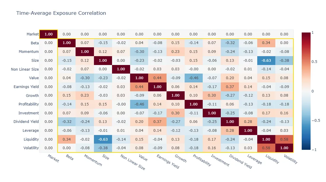
factor_model.plot_exposure_correlation(families=["market", "style"])
```
In the [example](#factor-model-code-example), the market exposure is constant
(every asset has unit exposure), so its correlation row is uninformative and
displays as zero. Market neutrality is instead guaranteed by benchmark-weighted
centering: every exposure has a zero benchmark-weighted mean, so no factor
carries net market exposure. The volatility-beta correlation and the correlation
between non-linear size and size are zero, as expected from the neutralization.
The remaining correlations are moderate, indicating no redundant factors. The
`families` argument excludes the 44 industry factors for readability. When
included, their correlations with the style factors are zero as well, the result
of within-industry scoring through `transform_by_group="industry"`, and the
industry-industry correlations are slightly negative rather than zero. Each asset
belongs to exactly one industry, so membership in one industry rules out
membership in all others. Zero correlation would mean industry memberships are
independent, while this exclusion is a negative relationship.
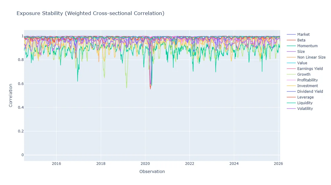
[`plot_exposure_stability`](https://skfolio.org/generated/skfolio.prior.FactorModel.html.md#skfolio.prior.FactorModel.plot_exposure_stability) shows the
cross-sectional correlation of each factor’s exposures between observations
with `step` determining how far apart the observations are sampled (21 by default).
Slow-moving factors (e.g. value, size) should stay highly correlated at a monthly
step. Fast-turnover factors (e.g. reversal, short-term momentum) reshuffle quickly
by construction and naturally show lower stability at that horizon. It is therefore
recommended to assess these factors with a shorter `step` (e.g. 1 to 5 days).
```python
factor_model.plot_exposure_stability(families=["market", "style"])
```
In the [example](#factor-model-code-example), monthly stability stays above
0.8 for nearly all factors and dates, with short-lived dips during stress
episodes (e.g. March 2020). Stable exposures keep the risk decomposition
consistent between rebalancings and limit the turnover induced by exposure noise.
[`FactorModel`](https://skfolio.org/generated/skfolio.prior.FactorModel.html.md#skfolio.prior.FactorModel) provides additional exposure diagnostics:
* [`plot_exposure_vif`](https://skfolio.org/generated/skfolio.prior.FactorModel.html.md#skfolio.prior.FactorModel.plot_exposure_vif)
* [`plot_exposure_condition_number`](https://skfolio.org/generated/skfolio.prior.FactorModel.html.md#skfolio.prior.FactorModel.plot_exposure_condition_number)
* [`plot_exposure_distribution`](https://skfolio.org/generated/skfolio.prior.FactorModel.html.md#skfolio.prior.FactorModel.plot_exposure_distribution)
* [`plot_exposure_dispersion`](https://skfolio.org/generated/skfolio.prior.FactorModel.html.md#skfolio.prior.FactorModel.plot_exposure_dispersion)
## Cross-Sectional Regression
After factor exposures are computed, the cross-sectional regression uses the
exposure tensor of shape `(n_observations, n_assets, n_factors)` together with
the asset return matrix of shape `(n_observations, n_assets)`. For each
observation, the model estimates factor returns and idiosyncratic returns by
regressing the cross-section of asset returns on the corresponding lagged exposures.
### Regression Model
For each observation $t$, factor returns solve the weighted least squares
problem:
$$
\hat{f}(t) = \arg\min_{f} \sum_{i} w_i(t)\,
\big(R_i(t) - B_i(t - \ell)^\top f\big)^2
$$
where $w_i(t)$ are the weights described in
[Regression Weights](#factor-model-regression-weights),
$B_i(t - \ell)$ is asset $i$’s lagged exposure vector and $\ell$ is
`exposure_lag`. Idiosyncratic returns are obtained as the regression residuals:
$$
\hat{\epsilon}_i(t) = R_i(t) - B_i(t - \ell)^\top \hat{f}(t)
$$
The regression is performed by `cs_regressor`, defaulting to
[`CSLinearRegression`](https://skfolio.org/generated/skfolio.linear_model.CSLinearRegression.html.md#skfolio.linear_model.CSLinearRegression), a weighted least-squares
estimator that solves all observations in one vectorized pass over the exposure
tensor. For robust or regularized cross-sectional estimation, skfolio allows
scikit-learn-compatible estimators (e.g. `HuberRegressor` for outlier-robust
regression) to be passed through
[`CSLinearRegressorWrapper`](https://skfolio.org/generated/skfolio.linear_model.CSLinearRegressorWrapper.html.md#skfolio.linear_model.CSLinearRegressorWrapper), which applies the
wrapped estimator separately to each observation.
#### NOTE
Unlike factor exposures, which are typically winsorized and standardized by
the exposure estimators, asset returns enter the cross-sectional regression
unadjusted. Cleaning return data errors is an upstream responsibility, since
the same returns drive benchmark weights, realized performance and downstream
optimization. Winsorizing legitimate extreme returns would break the
reconciliation of $R = B\,f + \epsilon$ and understate idiosyncratic
risk for heavy-tailed assets. Extreme observations are already moderated by
regression weights (`regression_mcap_power` and `inv_idio_variance_weight_shrinkage`).
When the factor-return regression needs to further reduce the influence of extreme
asset returns, use a robust regressor such as `HuberRegressor` through
[`CSLinearRegressorWrapper`](https://skfolio.org/generated/skfolio.linear_model.CSLinearRegressorWrapper.html.md#skfolio.linear_model.CSLinearRegressorWrapper) as described above.
### Regression Weights
Idiosyncratic returns are heteroskedastic, meaning idiosyncratic variance differs widely
across the cross-section. An unweighted regression would give excessive influence to the
noisiest names. Under heteroskedasticity, the best linear unbiased estimator (BLUE) is the
weighted least squares regression whose weights are proportional to inverse idiosyncratic
variance, known as generalized least squares (GLS).
Idiosyncratic variances are not observable before the regression is run. It is common practice
to approximate the inverse-variance weights with square-root market-cap weights (empirically,
idiosyncratic variance decreases roughly as the inverse square root of market capitalization).
The `regression_mcap_power` parameter controls this weighting as a power
$p$ of market capitalization:
$$
w_i \propto \mathrm{mcap}_i^{\,p}
$$
with `0.5` (default) for square-root cap weighting, `0.0` for equal weighting and
`1.0` for cap weighting. Market cap moves with the return being regressed,
$\mathrm{mcap}_i(t) \approx \mathrm{mcap}_i(t-1)\,(1 + R_i(t))$, and
weighting the regression at $t$ by caps at $t$ would correlate the
weights with the regressed returns and bias the estimated factor returns.
Because of this, market caps are also lagged by `exposure_lag`.
The model also supports inverse-idiosyncratic-variance weighting with a two-step
feasible GLS. A first pass runs with the cap-based weights and then the variances
estimated from its residuals (up to $t - 1$ only) feed the weights of the
second pass. The regression weights never depend on their own output, avoiding
the feedback loop of recursive weighting schemes where a low estimated variance
increases an asset’s weight and, in turn, its influence on later residuals.
`inv_idio_variance_max_weight_ratio` (default 20) caps each inverse-variance
weight at a multiple of the cross-sectional median, preventing assets with very
low estimated variance from dominating the regression.
Estimated variances are noisy, and `inv_idio_variance_weight_shrinkage` blends
the two weightings for robustness:
$$
w_i = \lambda\,w_i^{\text{inv-var}} + (1 - \lambda)\,w_i^{\text{cap}}
$$
where $\lambda = 0$ (default) uses the cap-based weights only and
$\lambda = 1$ the inverse-variance weights only.
The weights used at each date are stored in `factor_model_.regression_weights`: row
$t$ holds the weights used by the regression at $t$, built from market
caps at $t - \ell$ and idiosyncratic variances estimated up to $t - 1$.
### Zero-Sum Constraints
One-hot factor families are exactly collinear with the global factor: each
asset’s industry exposures sum to one, which is the global exposure. Including
both leaves the factor returns unidentified as adding a constant to every industry
return and subtracting it from the global return leaves the fit unchanged, and
the exposure design is rank-deficient.
The `constrained_families` parameter resolves this by imposing a benchmark-weighted
zero-sum constraint on the factor returns of each constrained family. Economically,
the global factor captures the benchmark portfolio return and the constrained family
factors capture relative effects around it.
Each tuple `(family, factor_to_drop)` specifies a family to reparameterize.
Instead of solving a constrained regression, the model applies an equivalent
change of basis. For a constrained family with exposure columns $x_j$ and
factor returns $\beta_j$, the constraint reads
$\sum_j w_j \beta_j = 0$, where $w_j$ is the benchmark weight
aggregated per factor (for one-hot industries, the benchmark weight of each
industry). Solving the constraint for one factor $k$ and substituting into
the regression yields an unconstrained regression on transformed features
$z_j$, with the dropped factor’s return reconstructed from the constraint
after fitting:
$$
z_j = x_j - \frac{w_j}{w_k}\,x_k,
\qquad
\hat{\beta}_k = -\frac{1}{w_k} \sum_{j \neq k} w_j \hat{\beta}_j
$$
The full family is reported with no loss of information, and all downstream
computations such as the factor covariance estimator and the
[regression diagnostics](#factor-model-regression-diagnostics) (t-statistics,
VIF, condition number, adjusted $R^2$) operate on a full-rank design.
Any choice of $k$ yields the same constrained solution. When `factor_to_drop` is `None`,
the model drops the factor with the largest $|w_k|$, keeping the ratios
$|w_j / w_k|$ bounded by 1.0 for most factors and preserving the
conditioning of the reduced design. The basis is stored in
`factor_model_.family_constraint_basis` and follows the same timing as the
regression. Realized factor returns are reconstructed with the lagged ratios used
by the regression, while expected factor returns and covariance are expanded with
the latest as-of basis.
### Global Factor and Benchmark Portfolio
Under the exposure centering and zero-sum constraints described in
[Zero-Sum Constraints](#factor-model-zero-sum-constraints), the global
factor return captures the benchmark portfolio return. Aggregating the
cross-sectional regression over the assets $i$ of the estimation
universe under benchmark weights gives (time indices omitted):
$$
\underbrace{\sum_i w_i^{\text{bench}} R_i}_{\text{benchmark return}}
= \hat{f}_0
+ \underbrace{\sum_{j \in \text{industry, country}} w_j\,\hat{f}_j}_{=\,0
\text{ (zero-sum constraint)}}
+ \sum_{j \in \text{styles}} \underbrace{\Big(\sum_i w_i^{\text{bench}}
B_{ij}\Big)}_{=\,0 \text{ (benchmark-centered)}} \hat{f}_j
+ \underbrace{\sum_i w_i^{\text{bench}}\,\hat{\epsilon}_i}_{\approx\,0}
$$
where $\hat{f}_0$ is the global factor return, $\hat{f}_j$ the
other factor returns, $B_{ij}$ the exposure of asset $i$ to factor
$j$ and $\hat{\epsilon}_i$ its idiosyncratic return.
* For a constrained one-hot family such as industry or country, the benchmark
exposure to factor $j$ is the total benchmark weight of the assets in
that category, $w_j = \sum_i w_i^{\text{bench}} B_{ij}$ (the industry
cap share when `benchmark_mcap_power=1`). The family term
$\sum_j w_j \hat{f}_j$ is the benchmark-weighted average of the
family’s factor returns, set to zero by the zero-sum constraint.
* Style exposures are centered so that the benchmark-weighted average
exposure $\sum_i w_i^{\text{bench}} B_{ij}$ is zero (the default
[`CSStandardScaler`](https://skfolio.org/generated/skfolio.preprocessing.CSStandardScaler.html.md#skfolio.preprocessing.CSStandardScaler) behavior). The benchmark
has no style tilt and style factor returns do not contribute to its
return.
* The residual term is the benchmark-weighted average of the idiosyncratic
returns. The weighted residuals sum to zero under the regression weights,
and the remaining difference between benchmark and regression weights is
diversified across the cross-section.
The estimated global factor return tracks the benchmark portfolio return on
the estimation universe (e.g. the market-cap portfolio when
`benchmark_mcap_power=1`), with deviations limited to the residual term when
regression weights differ from benchmark weights. When
`regression_mcap_power == benchmark_mcap_power` and
`inv_idio_variance_weight_shrinkage == 0`, the regression weights are
proportional to the benchmark weights and the residual term is exactly zero:
the WLS normal equations make the weighted residuals orthogonal to every
column of the exposure design, including the global column of ones, so
$\sum_i w_i^{\text{bench}} \hat{\epsilon}_i = 0$ and the identity is
exact:
$$
\hat{f}_0(t) = \sum_i w_i^{\text{bench}}\,R_i(t)
$$
The benchmark weights are stored in `factor_model_.benchmark_weights`. Under this
structure, each factor return reads as a portfolio return relative to the
benchmark. The global factor is the benchmark return itself. An industry factor
return is a benchmark-relative industry effect meaning it captures the return earned by that industry
in excess of the benchmark, net of the other factors. A style factor return is the
return to a standardized characteristic tilt, representing the return earned by holding one
standard deviation of exposure to that characteristic while keeping all other
factor exposures at zero.
### Missing Data and Changing Universes
Because the regression is re-estimated independently at each date, changing universes
are handled naturally, with newly listed assets joining the regression as soon as their
exposures are available, delisted assets dropping out, and assets on holiday
excluded for that date only. No realignment or imputation is needed.
At each date, an asset participates in the regression when it belongs to the
estimation universe and its lagged exposures and return are finite. All other pairs
receive zero regression weight. Assets outside the estimation universe still receive
exposures, idiosyncratic returns and forecasts where computable.
As a guard against underspecified regressions, `min_regression_assets` sets the
minimum number of participating assets required at every observation after the
[warmup period](#factor-model-warmup) (default
`max(2 * n_factors, 30)`). A ValueError is raised when a cross-section falls below
this minimum.
### Currency Factors
In a multi-currency universe, asset returns in the investor’s numeraire mix equity
risk with currency risk. The model separates the two components by estimating non-currency
factors from local excess returns and adding currency risk through dedicated currency factors.
The `currency_factor` parameter takes a one-hot exposure estimator on the asset currency
field (typically [`OneHotCategoricalFactors`](https://skfolio.org/generated/skfolio.factor_exposure.OneHotCategoricalFactors.html.md#skfolio.factor_exposure.OneHotCategoricalFactors)),
and the `currency_excess_returns` argument of `fit` supplies the currency excess return
series. The base-currency excess return of asset $i$ decomposes as:
$$
R^{excess,base}_i(t) = R^{excess,local}_i(t) + R^{ccy}_{C_i(t)}(t)
$$
where $R^{excess,local}_i(t)$ is the asset’s local-currency return in
excess of the cash rate of its currency $C_i(t)$ and
$R^{ccy}_{C_i(t)}(t)$ is the currency excess return from converting that
local-currency asset return into the investor’s base currency:
$$
R^{ccy}_{C_i(t)}(t) = R^{FX}_{C_i(t)}(t) + r^{cash}_{C_i(t)}(t)
- r^{cash}_{base}(t) + R^{local}_i(t)\,R^{FX}_{C_i(t)}(t)
$$
The identity follows from compounding the local return with the FX return and
subtracting the cash rates defining each excess return (time indices omitted):
$$
R^{base}_i &= (1 + R^{local}_i)(1 + R^{FX}_{C_i}) - 1
= R^{local}_i + R^{FX}_{C_i} + R^{local}_i\,R^{FX}_{C_i} \\
R^{excess,base}_i &= R^{base}_i - r^{cash}_{base} \\
&= \big(R^{local}_i - r^{cash}_{C_i}\big)
+ R^{FX}_{C_i} + r^{cash}_{C_i} - r^{cash}_{base}
+ R^{local}_i\,R^{FX}_{C_i} \\
&= R^{excess,local}_i + R^{ccy}_{C_i}
$$
The currency excess return series are computed by the user and supplied through
`currency_excess_returns`, with one column per currency factor.
Unlike equity factor returns, currency factor returns are not estimated by the
regression but instead are observed FX series in the investor’s numeraire which are then
appended directly to the factor return distribution with family `"currency"`. The factor
covariance then captures both equity and currency factor risk, and each asset loads
on its currency through the one-hot exposures.
### Regression Diagnostics
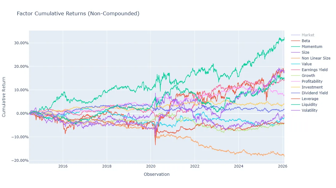
[`plot_factor_cumulative_returns`](https://skfolio.org/generated/skfolio.prior.FactorModel.html.md#skfolio.prior.FactorModel.plot_factor_cumulative_returns) displays the
estimated factor returns accumulated through time:
```python
fig = factor_model.plot_factor_cumulative_returns(families=["market", "style"])
```
Summary statistics of the style factors from the fitted model:
```python
factor_model.summary(families="style")[
["annualized_mean", "annualized_vol", "annualized_sharpe", "mean_vif"]
]
```
annualized_mean
annualized_vol
annualized_sharpe
mean_vif
beta
0.015
0.056
0.265
1.530
momentum
0.028
0.044
0.622
1.461
size
0.016
0.041
0.385
3.658
non_linear_size
-0.016
0.019
-0.833
1.518
value
-0.001
0.019
-0.072
2.324
earnings_yield
0.012
0.023
0.530
1.958
growth
-0.004
0.016
-0.228
1.330
profitability
0.007
0.015
0.443
1.814
investment
0.003
0.011
0.294
1.256
dividend_yield
0.002
0.015
0.114
1.518
leverage
-0.004
0.016
-0.225
1.248
liquidity
0.012
0.032
0.379
4.587
volatility
-0.001
0.032
-0.046
1.900
In the [example](#factor-model-code-example), momentum carries the highest
annualized Sharpe ratio (0.62) and the largest cumulative return, with the sharp
2020 reversal characteristic of momentum crashes. The beta, size, earnings yield
and profitability factors show positive premia over the sample while value is
flat. The mean VIFs are all below 5, consistent with the moderate exposure
correlations observed in [Exposure Diagnostics](#factor-model-diagnostics).
#### NOTE
These are pure-factor returns, not sorted long-short factor portfolio returns
such as the Fama-French factors. Their numerical scale is generally smaller
than that of familiar academic factor portfolios. Each factor return can be
interpreted as the return of a factor-mimicking portfolio constructed by the
cross-sectional regression. This portfolio is not rescaled to a fixed gross
exposure or volatility, whereas academic factors are often constructed as
100% long and 100% short (200% gross exposure) and may carry several units
of factor exposure together with incidental exposures to other factors.
Factor-return series should therefore only be compared after matching
exposure scaling and portfolio normalization conventions. Sharpe ratios are
more comparable because rescaling changes the mean and volatility proportionally.
In a characteristics factor model, each factor return is the cross-sectional
regression coefficient for one unit of exposure. For style factors built from
standardized exposures, this corresponds to one cross-sectional standard
deviation of exposure after winsorization, within-industry scoring and
neutralization. Equivalently, the factor-mimicking portfolio has unit
exposure to that factor and zero exposure to the other factors.
Factor-return signs follow the exposure convention. The size factor is built
from `LogMarketCap`, so a positive size factor return means large-cap
exposure was rewarded, the opposite of the Fama-French small-minus-big
convention. The sign convention only matters when comparing to external
factor series and it does not affect covariance decomposition, attribution or
optimization because exposures and factor returns are used consistently
within the model.
[`cs_regression_scores`](https://skfolio.org/generated/skfolio.prior.FactorModel.html.md#skfolio.prior.FactorModel.cs_regression_scores) returns per-observation
fit statistics: `r2`, `adjusted_r2` (adjusted for the effective number of
regressors, reduced when constraints are active), `aic` and `bic`.
```python
factor_model.cs_regression_scores.mean()
```
```text
r2 0.312856
adjusted_r2 0.278087
aic -10183.548079
bic -9894.130723
```
[`plot_cs_regression_scores`](https://skfolio.org/generated/skfolio.prior.FactorModel.html.md#skfolio.prior.FactorModel.plot_cs_regression_scores) displays them
through time:
```python
factor_model.plot_cs_regression_scores(score="adjusted_r2", window=20)
```
The mean $R^2$ is an in-sample quantity and does not account for model
complexity or overfitting, making it a weak measure of model quality. It does however
remain useful as a sanity check. For daily US equity models, the mean $R^2$ typically
falls between 25% and 40% and the mean adjusted $R^2$ between 20% and 35%.
Values outside these ranges typically warrant investigation. Three caveats apply:
* A mean $R^2$ of 30% does not mean the model explains only 30% of portfolio risk:
the daily cross-sectional $R^2$ is an in-sample fit statistic for that
day’s stock returns, while a portfolio’s risk can still be dominated by common
factors because idiosyncratic terms diversify away and factor terms do not.
* Some vendors report $R^2$ on monthly returns, which is mechanically higher than
on daily returns, and figures are only comparable at the same frequency.
* $R^2$ should not be used to compare different models as the addition of any
factor will lead to a larger value.
[`cs_regression_t_stats`](https://skfolio.org/generated/skfolio.prior.FactorModel.html.md#skfolio.prior.FactorModel.cs_regression_t_stats) returns the
per-observation t-statistic of each factor return, computed in the reduced basis
when constraints are active. Values of $|t| > 2$ indicate significance at
approximately the 5% level.
[`plot_cs_regression_t_stats`](https://skfolio.org/generated/skfolio.prior.FactorModel.html.md#skfolio.prior.FactorModel.plot_cs_regression_t_stats) displays them
through time.
[`cs_regression_t_stat_exceedance_rate`](https://skfolio.org/generated/skfolio.prior.FactorModel.html.md#skfolio.prior.FactorModel.cs_regression_t_stat_exceedance_rate)
aggregates this through time. A factor whose true coefficient is zero would
exceed the threshold about 5% of the time. Rates persistently above this
reference indicate a factor that is repeatedly significant in the cross-section.
[`plot_cs_regression_t_stat_exceedance_rate`](https://skfolio.org/generated/skfolio.prior.FactorModel.html.md#skfolio.prior.FactorModel.plot_cs_regression_t_stat_exceedance_rate)
displays the exceedance rates:
```python
factor_model.plot_cs_regression_t_stat_exceedance_rate(families=["market", "style"])
```
## Risk Forecasting
The risk forecast combines the distribution of factor returns and the idiosyncratic risk of each asset.
This section details their estimation and how they are assembled into the asset covariance and
return scenarios.
### Factor Return Distribution
The estimated factor return time series is passed to `factor_prior_estimator`, a
[prior estimator](https://skfolio.org/user_guide/prior.html.md#prior) that produces the expected factor returns (factor
premia), the factor covariance and factor return scenarios. When zero-sum constraints
are present, the estimation runs in the reduced full-rank basis, making the factor
covariance positive definite by construction.
The default is [`EmpiricalPrior`](https://skfolio.org/generated/skfolio.prior.EmpiricalPrior.html.md#skfolio.prior.EmpiricalPrior) with
[`EWMu`](https://skfolio.org/generated/skfolio.moments.EWMu.html.md#skfolio.moments.EWMu) for expected returns and
[`RegimeAdjustedEWCovariance`](https://skfolio.org/generated/skfolio.moments.RegimeAdjustedEWCovariance.html.md#skfolio.moments.RegimeAdjustedEWCovariance) for covariance. The latter
addresses two known weaknesses of plain exponentially weighted covariance:
* It applies a scalar regime multiplier (Short-Term Volatility Update) that improves
risk calibration when volatility regimes change faster than the EWMA half-life can
track.
* It supports separate half-lives for variance and correlation. Empirically,
volatility mean-reverts faster than correlation: a shorter variance half-life adapts
quickly to volatility shifts while a longer correlation half-life reduces
estimation noise on co-movements.
It also supports optional Newey-West HAC correction through `hac_lags` to adjust for
serial correlation in factor returns.
Because the factor return series is low-dimensional ($K \ll N$), estimators
that would be unstable or expensive on thousands of assets are cheap and reliable on
factors. The factor prior is fully replaceable, e.g. covariance shrinkage or denoising can
be applied at the factor level, and views on factors can be expressed by using
[`EntropyPooling`](https://skfolio.org/generated/skfolio.prior.EntropyPooling.html.md#skfolio.prior.EntropyPooling) or [`OpinionPooling`](https://skfolio.org/generated/skfolio.prior.OpinionPooling.html.md#skfolio.prior.OpinionPooling) as
`factor_prior_estimator`. The factor return scenarios produced here feed
scenario-based risk measures (e.g. CVaR) downstream.
[`plot_factor_forecast_correlation`](https://skfolio.org/generated/skfolio.prior.FactorModel.html.md#skfolio.prior.FactorModel.plot_factor_forecast_correlation) shows the
factor return correlation forecast from the fitted factor covariance. High values
flag factors whose returns move together and carry overlapping risk. Industry
factors are omitted below for readability:
```python
factor_model.plot_factor_forecast_correlation(families=["market", "style"])
```
In the [example](#factor-model-code-example), most correlations are
moderate, indicating that the factors capture distinct risk dimensions. The 0.80 market-beta
correlation is the known exception. The beta factor return is the
reward for holding high-beta names over low-beta names, a spread that widens in
rising markets and reverses in falling markets, making it co-move with the market return
by construction. The two factors remain separated in the regression because their
exposures are near-orthogonal in the cross-section, and the co-movement of their
returns is captured by the factor covariance.
[`plot_factor_forecast_volatilities`](https://skfolio.org/generated/skfolio.prior.FactorModel.html.md#skfolio.prior.FactorModel.plot_factor_forecast_volatilities) shows each
factor’s annualized volatility forecast which is calculated as the square root
of the factor covariance diagonal. It ranks the factors by their standalone risk
contribution:
```python
factor_model.plot_factor_forecast_volatilities(families=["market", "style"])
```
The market factor dominates at close to 20% annualized volatility. Its return is
the benchmark return, while style factor returns are long-short spreads across
standardized exposures. The beta, momentum, size and liquidity factors form the
next tier around 5% to 8%, and the remaining styles sit near 2%.
### Idiosyncratic Risk
Per-asset idiosyncratic variances are estimated from the idiosyncratic returns by
`idio_variance_estimator`, defaulting to
[`RegimeAdjustedEWVariance`](https://skfolio.org/generated/skfolio.moments.RegimeAdjustedEWVariance.html.md#skfolio.moments.RegimeAdjustedEWVariance). The estimator must support
`partial_fit` so the model can recover per-asset variance estimates at each
observation, stored in `factor_model_.idio_variances`. Assets still in their
[warmup period](#factor-model-warmup) have NaN variances, which propagate
to the fitted moments and mark them as not yet investable.
A factor model assumes the factor structure captures all common risk, leaving
idiosyncratic returns uncorrelated across assets. The idiosyncratic covariance is
therefore diagonal by default. In practice, linked securities remain correlated
after the factor structure is removed (e.g. multiple share classes, ADRs versus
ordinary shares, or dual listings). Without correction, optimizers treat such
pairs as diversified sources of idiosyncratic risk and may over-allocate to them.
Correlation thresholding addresses these cases. When `idio_corr_threshold` is set to
$\tau > 0$, the `idio_corr_estimator` (defaulting to
[`EWCovariance`](https://skfolio.org/generated/skfolio.moments.EWCovariance.html.md#skfolio.moments.EWCovariance)) is fitted on idiosyncratic returns
standardized by their contemporaneous idiosyncratic volatility. Only the correlation
component of its output is retained: off-diagonal correlations with
$|\rho_{ij}| \le \tau$ are set to zero, and the surviving correlations are
recombined with the latest per-asset variances to form a sparse idiosyncratic
covariance. Variances and correlations are estimated separately because a single full
covariance estimator would mix per-asset variance estimation with off-diagonal
correlation noise. This keeps variances driven by `idio_variance_estimator` and
applies the correlation overlay only where residual correlations are large enough to
retain.
Persistent residual correlation across a broader group, such as sub-industry
peers under a coarse industry classification, signals a missing factor rather
than a thresholding problem. Adding the factor keeps the idiosyncratic covariance
sparse, while lowering $\tau$ to absorb the group reintroduces the
estimation noise the diagonal assumption avoids.
### Idiosyncratic Risk Calibration
These diagnostics test the idiosyncratic volatility forecasts through the
standardized idiosyncratic returns
$z_{it} = \epsilon_{it} / \hat\sigma_{it}$. Under correct calibration,
$z$ has cross-sectional standard deviation 1.0.
[`idio_calibration_summary`](https://skfolio.org/generated/skfolio.prior.FactorModel.html.md#skfolio.prior.FactorModel.idio_calibration_summary) aggregates the main
statistics:
* `mean_cs_std` close to 1.0 indicates correctly scaled idiosyncratic risk. Values
persistently above 1.0 indicate underestimated risk and persistently below 1.0
indicate overestimated risk.
* `mean_tail_rate_3sigma` is the fraction of standardized returns beyond three
standard deviations. The Gaussian reference is 0.27%, and values of 1% to 3% are
common for equity factor models due to fat tails.
* `mean_cs_excess_kurtosis` above zero and a moderate `mean_cs_skewness` are typical.
Two complementary statistics separate ranking power from calibration.
[`idio_vol_ic`](https://skfolio.org/generated/skfolio.prior.FactorModel.html.md#skfolio.prior.FactorModel.idio_vol_ic) is the Spearman correlation between
predicted volatility and the next-period absolute idiosyncratic return with high
values meaning that the model ranks cross-sectional volatility differences well.
[`idio_vol_residual_dependence`](https://skfolio.org/generated/skfolio.prior.FactorModel.html.md#skfolio.prior.FactorModel.idio_vol_residual_dependence) is the same
correlation after standardizing the next-period return by the predicted
volatility: under correct calibration it should be close to 0. The desirable
pattern is a high `idio_vol_ic` combined with residual dependence near 0.
[`plot_idio_calibration`](https://skfolio.org/generated/skfolio.prior.FactorModel.html.md#skfolio.prior.FactorModel.plot_idio_calibration) tracks the
cross-sectional standard deviation of the standardized returns through time:
```python
factor_model.plot_idio_calibration(window=20)
```
In the [example](#factor-model-code-example), the series oscillates around a
mean of 1.06, a slight average underestimation of idiosyncratic risk. The spike
above 1.5 at the COVID shock shows realized dispersion outrunning the forecasts,
followed by a dip below 0.7 as the variance estimator caught up while volatility
dissipated.
[`plot_idio_vol_ic`](https://skfolio.org/generated/skfolio.prior.FactorModel.html.md#skfolio.prior.FactorModel.plot_idio_vol_ic) displays the volatility rank
IC through time:
```python
factor_model.plot_idio_vol_ic()
```
The rolling mean holds near 0.4 across the sample: the model consistently
forecasts higher volatility for assets that subsequently realize larger
idiosyncratic moves. Together with the calibration series close to 1.0, the
idiosyncratic risk forecasts are both well ordered and well scaled.
[`FactorModel`](https://skfolio.org/generated/skfolio.prior.FactorModel.html.md#skfolio.prior.FactorModel) provides additional idiosyncratic risk
diagnostics:
* [`plot_idio_tail_rate`](https://skfolio.org/generated/skfolio.prior.FactorModel.html.md#skfolio.prior.FactorModel.plot_idio_tail_rate)
* [`plot_idio_kurtosis`](https://skfolio.org/generated/skfolio.prior.FactorModel.html.md#skfolio.prior.FactorModel.plot_idio_kurtosis)
* [`plot_idio_skewness`](https://skfolio.org/generated/skfolio.prior.FactorModel.html.md#skfolio.prior.FactorModel.plot_idio_skewness)
* [`plot_idio_vol_residual_dependence`](https://skfolio.org/generated/skfolio.prior.FactorModel.html.md#skfolio.prior.FactorModel.plot_idio_vol_residual_dependence)
### Asset Covariance Forecast
The asset covariance forecast assembles the pieces estimated above:
$$
\Sigma = B(T)\,F\,B(T)^\top + D
$$
where $B(T)$ is the latest loading matrix, $F$ the factor covariance
and $D$ the idiosyncratic covariance. The result is positive definite and
well conditioned by construction as the systematic part is low-rank positive
semidefinite and $D$ is positive diagonal (or sparse positive definite).
Asset return scenarios follow the same construction. Factor scenarios from the
factor prior are mapped through the latest loading matrix, and idiosyncratic
scenarios calibrated to the latest idiosyncratic risk forecast are added on top.
Optimizers using scenario-based risk measures (e.g. CVaR) therefore see both
return components.
skfolio exploits this structure when passing the asset covariance to downstream
optimizers. Portfolio variance splits into a factor contribution and an
idiosyncratic contribution:
$$
w^\top \Sigma\, w
= \lVert F^{1/2} B^\top w \rVert^2 + \lVert D^{1/2} w \rVert^2
$$
Both terms involve only small matrices: the $n \times K$ loading matrix,
the $K \times K$ factor covariance and the $n$ idiosyncratic
variances. skfolio’s convex optimizers build their risk constraints on these
directly, through `factor_model_.covariance_sqrt`, instead of assembling and
factorizing the dense $n \times n$ covariance. On a universe of thousands
of assets driven by a few dozen factors, this keeps the risk constraints small
and the optimization fast.
### Covariance Forecast Evaluation
In-sample fit does not measure forecast accuracy. The covariance forecast is
evaluated out of sample with
[`covariance_forecast_evaluation`](https://skfolio.org/generated/skfolio.model_selection.covariance_forecast_evaluation.html.md#skfolio.model_selection.covariance_forecast_evaluation) or, using online
learning for speed, [`online_covariance_forecast_evaluation`](https://skfolio.org/generated/skfolio.model_selection.online_covariance_forecast_evaluation.html.md#skfolio.model_selection.online_covariance_forecast_evaluation).
Both walk forward through the data, compare each covariance forecast with the
subsequently realized returns over an evaluation window and return a
[`CovarianceForecastEvaluation`](https://skfolio.org/generated/skfolio.model_selection.CovarianceForecastEvaluation.html.md#skfolio.model_selection.CovarianceForecastEvaluation) with summary
statistics and plots. Four diagnostics are computed:
* The **Mahalanobis calibration ratio** tests the full covariance structure across
all eigenvalue directions. The target is 1.0, with values above 1.0 indicating
underestimated risk and below 1.0 indicating overestimated risk.
* The **diagonal calibration ratio** applies the same test to individual asset
variances, ignoring correlations.
* The **portfolio bias statistic** tests covariance calibration along
user-supplied portfolio directions. For each test portfolio, realized
portfolio returns are divided by their forecast volatility, and the standard
deviation of that standardized series should be 1.0 under correct
calibration. Evaluating several representative portfolios can reveal
direction-specific under or over-estimated risk.
* The **portfolio QLIKE** scores portfolio variance forecasts, with lower values
indicating better forecasts.
The figures below evaluate the model with
[`online_covariance_forecast_evaluation`](https://skfolio.org/generated/skfolio.model_selection.online_covariance_forecast_evaluation.html.md#skfolio.model_selection.online_covariance_forecast_evaluation) and
`test_size=5`:
```python
from skfolio.model_selection import online_covariance_forecast_evaluation
evaluation = online_covariance_forecast_evaluation(
model,
X,
params={"characteristics": characteristics},
warmup_size=2 * 252 + 21,
test_size=5,
)
evaluation.plot_calibration()
```
In the [example](#factor-model-code-example), the diagonal ratio and the bias
statistic oscillate around the target, implying individual asset variances and
test-portfolio volatilities are well scaled. The Mahalanobis ratio stays near 1.5,
indicating that the remaining underestimation is concentrated in the covariance’s
low-variance directions. The Mahalanobis distance gives more weight to errors in
those directions, while the diagonal ratio and portfolio bias statistic are less
sensitive to them. All three ratios spike at the 2020 shock. The diagonal ratio and
bias statistic then fall below 1.0 through 2021 as the forecasts lag the post-crisis
decline in volatility, while the Mahalanobis ratio falls back toward its target
without crossing it. This low-variance underestimation originates mostly in the
idiosyncratic block (residual correlations and missing factors) and is addressed
with `idio_corr_threshold` and the optimizer-level regularization covered in
[Orthogonal Space Regularization](#factor-model-orthogonal-space-regularization).
The summary table aggregates the four diagnostics over the full evaluation
period:
```python
evaluation.summary()
```
mean
median
std
p5
p95
mad_from_target
target
Mahalanobis ratio
1.505
1.320
0.789
0.672
2.969
0.606
1.000
Diagonal ratio
1.087
0.921
0.817
0.349
2.207
0.453
1.000
Portfolio standardized returns
0.096
0.140
0.917
-1.545
1.360
0.695
mean=0, std=1
Portfolio QLIKE
-6.411
-6.696
1.700
-7.919
-4.387
lower is better
[`CovarianceForecastEvaluation`](https://skfolio.org/generated/skfolio.model_selection.CovarianceForecastEvaluation.html.md#skfolio.model_selection.CovarianceForecastEvaluation) provides
additional plots:
* [`plot_qlike_loss`](https://skfolio.org/generated/skfolio.model_selection.CovarianceForecastEvaluation.html.md#skfolio.model_selection.CovarianceForecastEvaluation.plot_qlike_loss)
* [`plot_exceedance`](https://skfolio.org/generated/skfolio.model_selection.CovarianceForecastEvaluation.html.md#skfolio.model_selection.CovarianceForecastEvaluation.plot_exceedance)
[`CovarianceForecastComparison`](https://skfolio.org/generated/skfolio.model_selection.CovarianceForecastComparison.html.md#skfolio.model_selection.CovarianceForecastComparison) runs the same
evaluation over several models and aggregates the results for side-by-side
comparison. Missing data follows the panel conventions: only finite observations
contribute and inactive assets are excluded.
The comparison below contrasts two
[`RegimeAdjustedEWCovariance`](https://skfolio.org/generated/skfolio.moments.RegimeAdjustedEWCovariance.html.md#skfolio.moments.RegimeAdjustedEWCovariance) regime half-lives for the
factor prior: `regime_half_life=month` (21 trading days) against
`regime_half_life=quarter` (63 trading days), which reacts more slowly to
volatility regime shifts.
```python
from skfolio.model_selection import CovarianceForecastComparison
comparison = CovarianceForecastComparison(
[eval_month, eval_quarter],
names=["regime_half_life=month", "regime_half_life=quarter"],
)
comparison.plot_calibration(diagnostics=("bias",))
```
```python
comparison.plot_qlike_loss()
```
The shorter month half-life adapts faster, its bias statistic overshoots less at
the 2020 shock, recovers sooner from the 2021 over-forecast and its QLIKE loss is
lower through the 2020-2021 stress. In calm periods the two models are nearly
indistinguishable, and the summary table shows similar aggregate diagnostics, with
the month half-life slightly lower on mean QLIKE.
```python
comparison.summary()
```
estimator
regime_half_life=month
regime_half_life=quarter
mean
median
std
p5
p95
mad_from_target
target
mean
median
std
p5
p95
mad_from_target
target
Mahalanobis ratio
1.505
1.320
0.789
0.672
2.969
0.606
1.000
1.504
1.310
0.792
0.672
2.974
0.604
1.000
Diagonal ratio
1.087
0.921
0.817
0.349
2.207
0.453
1.000
1.080
0.896
0.964
0.319
2.292
0.470
1.000
Portfolio standardized returns
0.096
0.140
0.917
-1.545
1.360
0.695
mean=0, std=1
0.086
0.133
0.937
-1.586
1.324
0.690
mean=0, std=1
Portfolio QLIKE
-6.411
-6.696
1.700
-7.919
-4.387
lower is better
-6.346
-6.694
2.024
-7.896
-4.426
lower is better
[`CovarianceForecastComparison`](https://skfolio.org/generated/skfolio.model_selection.CovarianceForecastComparison.html.md#skfolio.model_selection.CovarianceForecastComparison) provides
additional plots:
* [`plot_calibration`](https://skfolio.org/generated/skfolio.model_selection.CovarianceForecastComparison.html.md#skfolio.model_selection.CovarianceForecastComparison.plot_calibration)
with full diagnostics (Mahalanobis, diagonal, bias)
* [`plot_exceedance`](https://skfolio.org/generated/skfolio.model_selection.CovarianceForecastComparison.html.md#skfolio.model_selection.CovarianceForecastComparison.plot_exceedance)
## Expected Returns
[`CharacteristicsFactorModel`](https://skfolio.org/generated/skfolio.prior.CharacteristicsFactorModel.html.md#skfolio.prior.CharacteristicsFactorModel) estimates expected asset returns
from factor premia and an optional alpha forecast. The factor prior estimates expected
factor returns, which are mapped to assets through their exposures. This section
explains how these estimates are used together and how they are evaluated.
### Expected Factor Returns
With `alpha_estimator=None` and the default `spanned_alpha_shrinkage=1`, expected
asset returns are determined entirely by the factor premia:
$$
\mu = B(T)\,\mu_f
$$
where $\mu_f$ holds the expected factor returns estimated by
`factor_prior_estimator` (see [Factor Return Distribution](#factor-model-factor-return-distribution)) and $B(T)$ is the latest
loading matrix. Each asset’s expected return is the sum of the premia of the
factors it is exposed to, weighted by its exposures.
### Information Coefficient
[`exposure_ic_summary`](https://skfolio.org/generated/skfolio.prior.FactorModel.html.md#skfolio.prior.FactorModel.exposure_ic_summary) measures the
cross-sectional correlation between factor exposures at $t$ and the forward
mean asset return from $t+1$ to $t+h$, where $h$ is the
`horizon` parameter. The default `correlation_method` computes the Spearman rank
IC, with Pearson IC weighted by the regression weights as the alternative. The
summary reports `mean_ic`, `std_ic`, `ic_ir` (mean over standard deviation) and
`hit_rate` per factor.
[`plot_cumulative_exposure_ic`](https://skfolio.org/generated/skfolio.prior.FactorModel.html.md#skfolio.prior.FactorModel.plot_cumulative_exposure_ic) shows the
cumulative IC through time:
```python
factor_model.plot_cumulative_exposure_ic(families=["market", "style"])
```
```python
factor_model.exposure_ic_summary(families=["market", "style"])
```
mean_ic
std_ic
ic_ir
hit_rate
market
-0.003
0.095
-0.029
0.495
beta
-0.004
0.169
-0.022
0.497
momentum
0.016
0.154
0.103
0.564
size
0.008
0.141
0.059
0.528
non_linear_size
0.008
0.124
0.063
0.532
value
-0.006
0.111
-0.057
0.459
earnings_yield
0.006
0.119
0.051
0.509
growth
0.005
0.068
0.075
0.548
profitability
0.011
0.098
0.117
0.552
investment
-0.000
0.067
-0.001
0.495
dividend_yield
0.004
0.125
0.031
0.505
leverage
-0.004
0.075
-0.052
0.475
liquidity
-0.010
0.155
-0.064
0.475
volatility
-0.010
0.132
-0.076
0.464
Daily ICs are small in absolute value, and the persistence of their sign matters
more than their level. In the [example](#factor-model-code-example),
momentum and profitability accumulate positive IC steadily across the sample
(hit rates of 56% and 55%), while volatility, liquidity and value accumulate
negative IC.
The IC quantifies return-predictive power. In a risk model, factors are designed
to forecast covariance, not expected returns. A factor can
therefore be an excellent risk factor with an IC near zero, and a low IC is not
a reason to discard it. IC is mainly useful for evaluating alpha signals and
factor premia, not for deciding whether a factor should remain in a risk model.
### Alpha Estimators
The `alpha_estimator` parameter accepts any [`BaseAlpha`](https://skfolio.org/generated/skfolio.alpha.BaseAlpha.html.md#skfolio.alpha.BaseAlpha)
estimator producing an expected-return forecast for each asset. Before it is fitted,
the factor model enriches the panel with the quantities it has already estimated:
idiosyncratic returns, idiosyncratic variances, regression weights, benchmark
weights and the factor exposure tensor. In typical alpha research workflows,
idiosyncratic returns serve as the prediction target (typically after
cross-sectional transformation), idiosyncratic variances scale the target and
factor exposures neutralize the features. Targeting idiosyncratic returns rather
than raw returns removes the factor-driven component from the target. The
cross-sectional variation of raw returns includes each asset’s factor exposures
multiplied by the factor returns, so a signal correlated with the exposures would
pick up factor premia already captured by the factor model. The idiosyncratic
target also carries less noise, since common factor volatility is removed.
The alpha forecast should be expressed in expected-return units when it is combined
with expected factor returns or used in an optimization alongside return-denominated
quantities (e.g. transaction costs, turnover constraints, return targets). Unitless
cross-sectional scores are appropriate only when the downstream objective treats
them as ordinal signals.
skfolio provides alpha estimators following the same signal pipeline as
factor exposures with descriptors being transformed into cross-sectional scores
(`outlier_transformer`, `scoring_transformer`, `transform_by_group`), optionally
neutralized against factor exposures (`neutralize_against`) and re-scored. The
estimators differ mainly in how the scored descriptors are combined and how the
result is scaled into expected-return units.
* [`FixedWeightedAlpha`](https://skfolio.org/generated/skfolio.alpha.FixedWeightedAlpha.html.md#skfolio.alpha.FixedWeightedAlpha) combines multiple descriptors
with fixed signed weights and a fixed `forecast_scale`. The weights define the
direction and relative contribution of each descriptor, while `forecast_scale`
converts one unit of composite score into the selected `forecast_unit`. This is useful
when the signal combination is specified outside the model and the main decision is
how strongly it should affect expected returns. `forecast_scale` requires careful
calibration as a value too large leads the optimizer to over-allocate to the alpha
forecast, whereas a value which is too small leaves the signal with little effect after
costs, risk limits and turnover constraints.
* [`EWSharpeOptimalAlpha`](https://skfolio.org/generated/skfolio.alpha.EWSharpeOptimalAlpha.html.md#skfolio.alpha.EWSharpeOptimalAlpha) combines descriptors linearly and
estimates their coefficients with exponentially weighted least squares on forward
idiosyncratic returns, using inverse idiosyncratic variance as regression weights.
It learns both sign and scale from realized data and accounts for cross-descriptor
correlations, scaling the signal blend according to its estimated idiosyncratic
return payoff. `forecast_scale` is then applied to the learned return-unit
forecast as a final strength multiplier. The learned coefficients are subject to
sampling error: short half-lives, noisy targets, weak descriptors and descriptors
whose predictive content is already absorbed by the factor model produce unstable
coefficients that can degrade an otherwise useful raw signal.
* [`PredictorAlpha`](https://skfolio.org/generated/skfolio.alpha.PredictorAlpha.html.md#skfolio.alpha.PredictorAlpha) wraps a user-provided
scikit-learn regressor and treats each observation-asset pair as one training sample.
It supports nonlinear interactions and non-additive signal effects, for example with
tree-based models or regularized regressors. With `calibrate_to_return_units=True`,
the raw predictor output is calibrated to expected-return units by exponentially
weighted least squares, so `alpha_` is in expected-return units.
`forecast_scale` is applied after this optional calibration. This flexibility
increases the need for robust validation, because nonlinear models can fit noise,
require more data and be sensitive to target construction and cross-validation
design.
All three estimators produce `alpha_` in expected-return units. The
`forecast_unit` parameter controls the unit of the intermediate forecast
([`ForecastUnit`](https://skfolio.org/generated/skfolio.alpha.ForecastUnit.html.md#skfolio.alpha.ForecastUnit)). With `ForecastUnit.IDIO_RETURN` (default),
the forecast is interpreted directly as expected idiosyncratic return. With
`ForecastUnit.IDIO_SHARPE`, the forecast is interpreted as idiosyncratic Sharpe and
multiplied by the current idiosyncratic volatility before being passed to the
factor model. The Sharpe unit is preferable when a signal is expected to rank
risk-adjusted opportunities rather than raw returns. `forecast_scale` is the
common final multiplier controlling alpha strength.
The following example combines two reversal descriptors, [`return on assets`](https://skfolio.org/generated/skfolio.descriptor.ReturnOnAssets.html.md#skfolio.descriptor.ReturnOnAssets),
and [`Amihud illiquidity`](https://skfolio.org/generated/skfolio.descriptor.EWAmihudIlliquidity.html.md#skfolio.descriptor.EWAmihudIlliquidity) with fixed signed weights and uses a Gaussian rank scorer
for the cross-sectional scoring:
```python
from skfolio.alpha import FixedWeightedAlpha
from skfolio.descriptor import EWAmihudIlliquidity, ReturnOnAssets, Reversal
from skfolio.preprocessing import CSGaussianRankScaler
alpha_estimator = FixedWeightedAlpha(
descriptors=[
("reversal_5d", Reversal(window=5)),
("reversal_21d", Reversal(window=21)),
("return_on_assets", ReturnOnAssets()),
("amihud_illiquidity", EWAmihudIlliquidity()),
],
weights=[1.0, 1.0, -1.0, -1.0],
forecast_scale=0.0001,
scoring_transformer=CSGaussianRankScaler(),
n_jobs=-1,
)
```
In practice, the simplest estimator that matches the research assumption is usually
the most robust starting point. Use [`FixedWeightedAlpha`](https://skfolio.org/generated/skfolio.alpha.FixedWeightedAlpha.html.md#skfolio.alpha.FixedWeightedAlpha)
when signal direction and relative weights are already specified and the main
decision is scale. Use [`EWSharpeOptimalAlpha`](https://skfolio.org/generated/skfolio.alpha.EWSharpeOptimalAlpha.html.md#skfolio.alpha.EWSharpeOptimalAlpha) when
the signal combination is expected to be approximately linear and there is enough
history to estimate stable payoffs. Use [`PredictorAlpha`](https://skfolio.org/generated/skfolio.alpha.PredictorAlpha.html.md#skfolio.alpha.PredictorAlpha)
when nonlinear effects are important and the additional validation burden is
acceptable. Custom estimators are created by subclassing
[`BaseAlpha`](https://skfolio.org/generated/skfolio.alpha.BaseAlpha.html.md#skfolio.alpha.BaseAlpha). During the alpha estimator’s
[warmup period](#factor-model-warmup), its forecast is treated as zero.
### Spanned and Orthogonal Alpha
The fitted alpha forecast is decomposed into spanned alpha and orthogonal alpha by
projecting it onto the factor exposure space with a weighted cross-sectional
regression, using the latest exposures and regression weights:
$$
\alpha = \alpha^{\parallel} + \alpha^{\perp}
\qquad \text{with} \qquad
\alpha^{\parallel} = B(T)\,g
$$
where $\alpha^{\parallel}$ is the spanned alpha,
$\alpha^{\perp}$ is the orthogonal alpha and $g$ is the factor-return
vector that reproduces the spanned alpha through $B(T)$.
`spanned_alpha_shrinkage` blends the factor-implied asset expected returns
$B(T)\,\mu_f$ with the spanned alpha:
$$
\mu^{\parallel}
= \lambda\,B(T)\,\mu_f + (1 - \lambda)\,\alpha^{\parallel}
$$
where $\mu_f$ contains expected factor returns estimated from the factor
return time series (see [Factor Return Distribution](#factor-model-factor-return-distribution)). $\lambda = 1$ (default) uses
factor-implied asset expected returns, $\lambda = 0$ uses the spanned alpha and
intermediate values blend the two. With the default, the alpha forecast contributes
to expected returns only through the orthogonal alpha.
The orthogonal alpha is shrunk towards zero by `orthogonal_alpha_confidence`:
$$
\mu = \mu^{\parallel} + c\,\alpha^{\perp}
$$
where $c = 1$ (default) uses the orthogonal alpha as-is and $c = 0$
discards it. Orthogonal directions are penalized only through idiosyncratic
variances in the covariance forecast, so an optimizer allocates to them
aggressively when they carry alpha. Reducing `orthogonal_alpha_confidence`
tempers this incentive when confidence in the forecast is limited.
[Orthogonal Space Regularization](#factor-model-orthogonal-space-regularization) covers this behavior and the
optimizer-level alternatives.
The shrunk orthogonal alpha $c\,\alpha^{\perp}$ is stored in
`factor_model_.idio_mu`. When currency factors are present, direct currency expected
returns are added to $\mu$.
With the default weighted least-squares cross-sectional regressor, the decomposition
satisfies $B(T)^\top W\alpha^{\perp}=0$. Custom robust or regularized
cross-sectional regressors may produce a component that is only approximately
orthogonal.
### Alpha and Risk Factor Alignment
A signal may closely resemble an existing risk-model factor while using a modified
definition that produces a stronger expected return. The key question is whether
the modified definition also provides a better representation of systematic risk.
If it explains common return variation better or improves risk forecasts, it should
replace the existing factor definition. Otherwise, the additional systematic
component would remain in idiosyncratic returns, causing the optimizer to underestimate
its risk.
If the modified definition improves expected returns but does not improve the risk
model, the existing risk factor should remain. The resulting alpha forecast can then
be decomposed into spanned alpha and orthogonal alpha. The orthogonal alpha is
diversifiable relative to the validated risk model, so allocating to it is intentional.
A historical example comes from momentum. Earlier commercial risk models measured
momentum over the most recent 12 months, including the latest month. Later
research separated medium-term momentum from short-term reversal by excluding
that latest month. A manager using the revised definition while retaining the older risk
model created a mismatch: the difference between the two definitions appeared
outside the modelled momentum factor and was treated as idiosyncratic risk. The optimizer
could therefore take a large position in that difference without accounting for its
systematic risk.
With skfolio, the definition can be tested directly and, when it provides a better
representation of systematic risk, used immediately in the risk model.
### Orthogonal Space Regularization
The factor structure has an asymmetric effect on the covariance forecast. Systematic
directions carry the full factor covariance, while directions orthogonal to the
factor span are penalized only through the per-asset idiosyncratic variances, since
the idiosyncratic covariance is diagonal or sparse. To an optimizer, orthogonal
directions therefore appear cheap in risk, and any orthogonal alpha makes them
attractive, leading to concentrated allocations in the orthogonal space.
If the model were correctly specified, complete and free of estimation error, this
behavior would be desirable as factor-neutral strategies (e.g. statistical arbitrage)
would exploit these directions. In practice the model is neither complete nor
error-free, so orthogonal risk is understated and some regularization is needed,
without giving up the orthogonal space entirely.
skfolio provides three mechanisms to achieve this. The first is a
[`CharacteristicsFactorModel`](https://skfolio.org/generated/skfolio.prior.CharacteristicsFactorModel.html.md#skfolio.prior.CharacteristicsFactorModel) parameter, the other two are
configured at the optimization step:
* `orthogonal_alpha_confidence` shrinks the orthogonal alpha point estimate toward
zero, reducing the incentive to allocate in orthogonal directions.
* [`OrthogonalMuUncertaintySet`](https://skfolio.org/generated/skfolio.uncertainty_set.OrthogonalMuUncertaintySet.html.md#skfolio.uncertainty_set.OrthogonalMuUncertaintySet), passed to the
optimizer’s `mu_uncertainty_set_estimator`, applies robust optimization to the
expected returns in the orthogonal space, penalizing allocations proportionally
to the uncertainty of the orthogonal alpha.
* [`OrthogonalCovarianceUncertaintySet`](https://skfolio.org/generated/skfolio.uncertainty_set.OrthogonalCovarianceUncertaintySet.html.md#skfolio.uncertainty_set.OrthogonalCovarianceUncertaintySet), passed to
the optimizer’s `covariance_uncertainty_set_estimator`, inflates the covariance
in orthogonal directions, raising their variance directly.
An optimizer can allocate in orthogonal directions even when the orthogonal alpha
is zero as binding constraints (e.g. factor-neutrality, long-only) act through
shadow prices and push weights into the orthogonal space. In a model without an
alpha estimator, such allocations carry idiosyncratic risk with no expected
reward, making the covariance-side regularization relevant beyond the alpha term
itself. The [Portfolio Construction](#factor-model-portfolio-construction)
section shows the optimizer-level configuration, and the regularization strength
(`radius`) can be selected by walk-forward evaluation or
[hyperparameter tuning](#factor-model-hyper-parameter-tuning).
### Alpha Forecast Diagnostics
Alpha research can be organized in two ways. The alpha estimator can either be developed
jointly with the factor model, attached through `alpha_estimator` and evaluated
end to end or it can be developed independently by first fitting a factor model without
an alpha estimator and then adding its fitted outputs to the panel with
[`enrich_asset_panel`](https://skfolio.org/generated/skfolio.prior.FactorModel.html.md#skfolio.prior.FactorModel.enrich_asset_panel) and finally iterating over
the alpha estimator directly using the enriched panel. The independent workflow avoids
refitting the factor model at each research iteration and is used below.
The [`alpha_forecast_evaluation`](https://skfolio.org/generated/skfolio.alpha.alpha_forecast_evaluation.html.md#skfolio.alpha.alpha_forecast_evaluation) function evaluates the
historical forecasts produced by an alpha estimator against a forward target
field in an [`AssetPanel`](https://skfolio.org/generated/skfolio.containers.AssetPanel.html.md#skfolio.containers.AssetPanel). The default target is
`idio_returns`, the part of returns not explained by the factor model. The
function fits the estimator with `fit_transform`, then compares the alpha
forecasts at observation $t$ with the forward mean target over
$[t + \ell, t + \ell + h)$, where $h$ is `holding_period` and
$\ell$ is `signal_lag`:
```python
from skfolio.utils.stats import CSWeighting
from skfolio.alpha import alpha_forecast_evaluation
characteristics_enriched = factor_model.enrich_asset_panel(characteristics)
evaluation = alpha_forecast_evaluation(
alpha_estimator,
characteristics_enriched,
holding_period=5,
signal_lag=1,
cs_weighting=CSWeighting.REGRESSION,
quantiles=(0.1, 0.25),
)
evaluation.ic_summary()
```
mean
std
icir
t_stat
hit_rate
spearman_ic
0.012
0.073
0.164
3.965
0.556
pearson_ic
0.009
0.068
0.135
3.255
0.539
```python
evaluation.portfolio_summary()
```
annualized_mean
annualized_vol
annualized_ir
hit_rate
mean_turnover
rank_weighted_portfolio
0.036
0.019
1.869
0.554
1.599
zscore_weighted_portfolio
0.037
0.022
1.710
0.552
1.745
The example alpha is deliberately simple. Its Spearman IC averages 0.012 with an
ICIR of 0.16 (t-stat 3.97) and a hit rate of 56%: a genuine but modest
predictive signal, in line with typical daily alpha signals. The simple
portfolios earn an annualized information ratio above 1.7 with substantial
turnover, gross of any trading friction. Whether such a signal can be monetized
depends on transaction costs, borrow costs, market impact and turnover
constraints, which enter at the optimization step and are covered in
[Portfolio Construction](#factor-model-portfolio-construction).
All diagnostics are computed on the final alpha forecast returned by the
estimator, after any rank transformation. With
`scoring_transformer=CSGaussianRankScaler()`, `spearman_ic` measures the ordering
quality of the forecast and `pearson_ic` the linear relation between
Gaussian-rank scores and future target returns. `zscore_weighted_portfolio` is
the simple portfolio closest to the expected-return vector consumed by an
optimizer, since the optimizer receives alpha values proportional to those
scores.
The [`AlphaForecastEvaluation`](https://skfolio.org/generated/skfolio.alpha.AlphaForecastEvaluation.html.md#skfolio.alpha.AlphaForecastEvaluation) result groups the diagnostics
as follows:
* [`ic_summary`](https://skfolio.org/generated/skfolio.alpha.AlphaForecastEvaluation.html.md#skfolio.alpha.AlphaForecastEvaluation.ic_summary): `spearman_ic`
measures ordering quality and is invariant to monotonic transformations of the
forecast. `pearson_ic`, weighted by `cs_weighting`, measures whether forecast
magnitudes are linearly related to realized targets.
* [`portfolio_summary`](https://skfolio.org/generated/skfolio.alpha.AlphaForecastEvaluation.html.md#skfolio.alpha.AlphaForecastEvaluation.portfolio_summary): annualized
statistics of alpha-only, gross-normalized long-short portfolios built from
centered ranks (`rank_weighted_portfolio`) or centered forecast values
(`zscore_weighted_portfolio`), before covariance, costs and constraints are
introduced by the optimizer.
* [`quantile_summary`](https://skfolio.org/generated/skfolio.alpha.AlphaForecastEvaluation.html.md#skfolio.alpha.AlphaForecastEvaluation.quantile_summary): annualized
top-minus-bottom target returns per tail quantile, showing whether predictive
content is concentrated in the tails.
* [`calibration_summary`](https://skfolio.org/generated/skfolio.alpha.AlphaForecastEvaluation.html.md#skfolio.alpha.AlphaForecastEvaluation.calibration_summary):
`calibration_slope` is the scale multiplier from a weighted zero-intercept
regression of realized target on forecast. A slope near 1.0 indicates the
forecast is already scaled to target units. Values above 1.0 indicate that
`forecast_scale` is too small, while values below 1.0 indicate that it is too
large.
* [`coverage_summary`](https://skfolio.org/generated/skfolio.alpha.AlphaForecastEvaluation.html.md#skfolio.alpha.AlphaForecastEvaluation.coverage_summary): fraction and
number of assets with finite forecast and target values. Low coverage can make
the other statistics unstable even when their averages look acceptable.
* [`factor_correlation_summary`](https://skfolio.org/generated/skfolio.alpha.AlphaForecastEvaluation.html.md#skfolio.alpha.AlphaForecastEvaluation.factor_correlation_summary):
contemporaneous cross-sectional correlation between the forecast and factor
exposures, testing whether the forecast is neutral to existing factors.
* [`decay_summary`](https://skfolio.org/generated/skfolio.alpha.AlphaForecastEvaluation.html.md#skfolio.alpha.AlphaForecastEvaluation.decay_summary) and
[`holding_period_summary`](https://skfolio.org/generated/skfolio.alpha.AlphaForecastEvaluation.html.md#skfolio.alpha.AlphaForecastEvaluation.holding_period_summary): IC and
simple-portfolio statistics across forward periods, showing whether the signal
is short-lived, persistent or delayed relative to the selected holding horizon.
Together, these diagnostics separate ordering quality from magnitude quality:
`spearman_ic` and `rank_weighted_portfolio` isolate the ordering, while
`pearson_ic`, `zscore_weighted_portfolio` and `calibration_summary` evaluate the
forecast values that an optimizer receives. `coverage_summary` checks data
availability and `decay_summary` aligns the alpha horizon with the intended
rebalancing and holding period. When the rank-based diagnostics are stronger
than the magnitude-based ones, the optimizer should not receive raw alpha
magnitudes as if they were calibrated expected returns.
```python
evaluation.plot_cumulative_ic()
```
```python
evaluation.plot_factor_correlation()
```
```python
evaluation.plot_cumulative_returns()
```
Both ICs accumulate steadily across the sample, with the strongest run in
2020-2021 and no prolonged negative stretch, indicating stable predictive power
rather than a few favorable periods. The factor correlation plot shows the
forecast is not fully factor-neutral as it carries a positive size correlation and
negative profitability and liquidity correlations, inherited from its
descriptors. If these tilts are unwanted, they can be removed with
`neutralize_against`. The simple portfolios compound consistently, with a sharp
drawdown and recovery around the COVID shock.
[`AlphaForecastEvaluation`](https://skfolio.org/generated/skfolio.alpha.AlphaForecastEvaluation.html.md#skfolio.alpha.AlphaForecastEvaluation) provides additional plots:
* [`plot_rolling_ic`](https://skfolio.org/generated/skfolio.alpha.AlphaForecastEvaluation.html.md#skfolio.alpha.AlphaForecastEvaluation.plot_rolling_ic)
* [`plot_quantile_returns`](https://skfolio.org/generated/skfolio.alpha.AlphaForecastEvaluation.html.md#skfolio.alpha.AlphaForecastEvaluation.plot_quantile_returns)
* [`plot_calibration`](https://skfolio.org/generated/skfolio.alpha.AlphaForecastEvaluation.html.md#skfolio.alpha.AlphaForecastEvaluation.plot_calibration)
* [`plot_ic_by_holding_period`](https://skfolio.org/generated/skfolio.alpha.AlphaForecastEvaluation.html.md#skfolio.alpha.AlphaForecastEvaluation.plot_ic_by_holding_period)
* [`plot_portfolio_by_holding_period`](https://skfolio.org/generated/skfolio.alpha.AlphaForecastEvaluation.html.md#skfolio.alpha.AlphaForecastEvaluation.plot_portfolio_by_holding_period)
* [`plot_ic_decay`](https://skfolio.org/generated/skfolio.alpha.AlphaForecastEvaluation.html.md#skfolio.alpha.AlphaForecastEvaluation.plot_ic_decay)
* [`plot_portfolio_decay`](https://skfolio.org/generated/skfolio.alpha.AlphaForecastEvaluation.html.md#skfolio.alpha.AlphaForecastEvaluation.plot_portfolio_decay)
When the diagnostics show reliable ordering but weak magnitude calibration, a
practical approach is to keep the alpha shape rank-based and control its strength
with a single scale parameter. For descriptor-composition estimators, this is
done with a rank-based `scoring_transformer` (e.g.
[`CSGaussianRankScaler`](https://skfolio.org/generated/skfolio.preprocessing.CSGaussianRankScaler.html.md#skfolio.preprocessing.CSGaussianRankScaler)), as in the
[`FixedWeightedAlpha`](https://skfolio.org/generated/skfolio.alpha.FixedWeightedAlpha.html.md#skfolio.alpha.FixedWeightedAlpha) example of the
[Alpha Estimators](#factor-model-alpha) section. The resulting alpha is
still in expected-return units:
$$
\alpha_i = s \, z_i
$$
where $z_i$ is the cross-sectional Gaussian rank score and $s$ is
`forecast_scale`. The rank transformation defines the relative shape of the forecast,
while `forecast_scale` maps one rank-normal score unit to expected-return units.
This unit conversion is important in mean-risk optimization as the optimizer trades off
expected return, risk, constraints and transaction costs in the same objective. If
transaction costs are expressed in return units, the alpha forecast must also be in
return units. A rank-based alpha satisfies this requirement once it is multiplied by
`forecast_scale`.
With a rank-based alpha, calibration reduces to choosing the scale. If
`forecast_scale` is too small, transaction costs and risk penalties may dominate the
signal and the optimizer will keep positions close to their starting weights. If it is
too large, the optimizer may overtrade the ranked signal. The `calibration_summary`,
`portfolio_summary` and `decay_summary` diagnostics help choose a scale that is
consistent with realized target returns and the expected holding horizon.
## Portfolio Construction
The factor model is a prior estimator and can be passed to any skfolio optimizer
through the `prior_estimator` parameter. The optimizer fits the
prior internally, then consumes its expected returns, covariance and scenarios.
The `characteristics` panel is forwarded to the prior through scikit-learn
metadata routing.
This section builds two portfolios on the fitted model: a factor-constrained
portfolio that trades factor premia through explicit exposure targets, and a
factor-neutral portfolio built from the orthogonal alpha.
### Factor-Constrained Portfolio
The example below builds a dollar-neutral long-short portfolio with positive
momentum and profitability exposures, together with a negative exposure to the
non-linear size factor. The exposure levels are chosen for illustration so their
effects remain clear in the later attribution analysis.
The -2.0 target for `non_linear_size` shows how factor constraints can express
more complex patterns than a simple large-versus-small tilt. The factor is built
as the cube of the size exposure and neutralized against size, which produces
the following approximate tilts:
| Size region | Portfolio tilt |
|------------------|------------------|
| Very small | Long |
| Moderately small | Short |
| Moderately large | Long |
| Very large | Short |
```python
from sklearn import set_config
from skfolio import RiskMeasure
from skfolio.optimization import MeanRisk, ObjectiveFunction
set_config(enable_metadata_routing=True)
X = characteristics.to_dataframe(fields="returns")
industry_names = characteristics.fields["industry"].levels
mvo = MeanRisk(
objective_function=ObjectiveFunction.MAXIMIZE_RATIO,
risk_measure=RiskMeasure.VARIANCE,
prior_estimator=model, # factor model as prior
max_weights=0.05, # limit individual positions to 5%
min_weights=-0.05, # allow short positions and limit to -5%
budget=0.0, # dollar neutral
max_long=1.0, # 100% long and 100% short: 200% gross exposure
transaction_costs=0.001 / month, # 10 bps amortized over one month
fallback="previous_weights", # keep last valid weights if a fit fails
linear_constraints=[
"momentum >= 1.0",
"profitability == 1.0",
"non_linear_size == -2.0",
# Exact neutrality
"beta == 0",
"size == 0",
"volatility == 0",
# Small bands on the remaining styles
"growth <= 0.05",
"growth >= -0.05",
"investment <= 0.05",
"investment >= -0.05",
"value <= 0.05",
"value >= -0.05",
"liquidity <= 0.05",
"liquidity >= -0.05",
"earnings_yield <= 0.05",
"earnings_yield >= -0.05",
"leverage <= 0.05",
"leverage >= -0.05",
"dividend_yield <= 0.05",
"dividend_yield >= -0.05",
# Industry neutrality
*[f"{name} == 0.0" for name in industry_names],
],
)
mvo.fit(X, characteristics=characteristics)
print(mvo.weights_)
# Factor model fitted inside the optimizer, reused below for attribution
factor_model = mvo.prior_estimator_.factor_model_
```
Here the full coverage universe serves as the investment universe: `X` contains
the returns of every asset in the panel. The factor model fitted inside the optimizer is
available through `mvo.prior_estimator_.factor_model_` and is reused in the
[Attribution](#factor-model-attribution) section. A separate factor model
can also be fitted for attribution only.
The portfolio is dollar neutral with `budget=0.0` and limited to 100% long
exposure with `max_long=1.0`. Dollar neutrality implies an equally sized short
position, so the maximum gross exposure is 200% (100% long plus 100% short).
Individual positions are limited to $\pm 5\%$. Transaction costs follow the
skfolio convention: a linear cost per unit traded, deducted from the portfolio
expected return, which is expressed per observation period (here daily). A
transaction cost is paid once per rebalancing while a position earns its return
on every period it is held, so the 10 basis points are amortized over the
one-month expected holding period to convert them to a daily cost,
`0.001 / month` (see
[Periodicity Convention](https://skfolio.org/user_guide/data_preparation.html.md#periodicity-convention)). Market
impact and borrow costs can be added through the optimizer’s `add_objective` and
`add_constraints` parameters, with native support planned for a future release.
The portfolio targets three equity styles: momentum, profitability and non-linear size.
The beta, size and volatility exposures are set to zero. The remaining styles are
constrained within $\pm 0.05$, and industry exposures are neutralized. In
`linear_constraints`, an expression on a factor name (e.g. `"momentum >= 1.0"`)
applies to the portfolio exposure to that factor, while an expression on a family
name (e.g. `"style <= 0.5"`) applies to the sum of exposures over the family’s
factors. Industry neutrality therefore uses one constraint per industry
factor rather than a single `"industry == 0"` constraint, which would only force
industry exposures to offset each other. No explicit
`"market == 0"` constraint is needed because `budget=0.0` already sets the
global factor exposure to zero.
`fallback="previous_weights"` keeps the latest valid allocation when a
rebalancing problem is infeasible, for example on dates where strict constraints
cannot be satisfied. Fallback estimators and the fallback audit trail are covered
in [Failure and Fallbacks](https://skfolio.org/auto_examples/mean_risk/plot_17_failure_and_fallbacks.html.md#sphx-glr-auto-examples-mean-risk-plot-17-failure-and-fallbacks-py).
The portfolio is evaluated using monthly walk-forward rebalancing:
```python
from skfolio.model_selection import online_predict
# Two years plus one month of observations warm up the model
# before the first rebalancing
warmup_size = 252 * 2 + 21
mpp = online_predict(
estimator=mvo,
X=X,
warmup_size=warmup_size,
test_size=month,
params={"characteristics": characteristics},
)
print(mpp.n_fallback_portfolios)
print(mpp.summary())
print(mpp.annualized_sharpe_ratio)
mpp.plot_cumulative_returns()
```
```python
mpp.plot_composition()
```
`online_predict` returns a [`MultiPeriodPortfolio`](https://skfolio.org/generated/skfolio.portfolio.MultiPeriodPortfolio.html.md#skfolio.portfolio.MultiPeriodPortfolio), one
portfolio per rebalancing. The [Portfolio](https://skfolio.org/user_guide/portfolio.html.md#portfolio) user guide covers the
portfolio objects and their analytics (e.g. `plot_long_short_exposure`,
`plot_contribution`, `summary`). The two-year `warmup_size` covers the stacked
descriptor and estimator warmups (see [Warmup Periods](#factor-model-warmup)). The out-of-sample portfolio achieves an annualized
Sharpe ratio of 0.91.
The optimizer consumes the factor model with the following conventions:
* For variance-based risk measures, the optimizer consumes the covariance square
root described in the [Asset Covariance Forecast](#factor-model-asset-covariance-forecast) section,
operating in the factor space instead of forming the dense asset covariance.
* For scenario-based risk measures (e.g. `RiskMeasure.CVAR`), the optimizer consumes
the asset return scenarios from `return_distribution_.returns`, which combine
factor and idiosyncratic components. With [online learning](#factor-model-online-learning), `max_history` keeps the
scenarios on a rolling window.
* Assets that are not investable at the current date (e.g. delisted, in warmup)
carry NaN moments. The optimizer solves on the investable subset and assigns them
zero weight, as described in the [Input Data](#factor-model-input-data) section.
Robust optimization in the orthogonal space is configured at the optimizer level,
following the [Orthogonal Space Regularization](#factor-model-orthogonal-space-regularization) section:
```python
from skfolio.uncertainty_set import OrthogonalCovarianceUncertaintySet
mvo.set_params(
covariance_uncertainty_set_estimator=OrthogonalCovarianceUncertaintySet(radius=1.0)
)
```
This example trades factor premia and does not use an alpha forecast. The
factor-neutral case is covered in the [Factor-Neutral Alpha Portfolio](#factor-model-factor-neutral-alpha-portfolio) section below.
Walk-forward evaluation and hyperparameter tuning of the full
optimization-plus-prior pipeline are covered in the [Walk-Forward Evaluation](#factor-model-walk-forward-evaluation) and [Hyperparameter Tuning](#factor-model-hyper-parameter-tuning) sections.
#### NOTE
When the research focus is the optimization itself and the factor model is
fixed, refitting the prior at each iteration can dominate the runtime on
large universes. The factor model outputs can be precomputed over the chosen
observations, stored in a database or local cache, and served back by a custom
prior estimator that reads them for the requested observation range. Native
factor model caching is planned for a future release.
### Factor-Neutral Alpha Portfolio
The previous example earns its return from factor premia through explicit
exposure targets. This portfolio keeps factor exposures close to zero and uses the
orthogonal alpha as its modeled expected return, an approach common in statistical
arbitrage. The orthogonal alpha is the residual of the alpha forecast after
projection onto the factor exposure space.
#### NOTE
A factor-neutral portfolio has zero exposure to every factor, so its modeled
expected return reduces to the orthogonal alpha. Without an alpha estimator,
the orthogonal alpha is zero and the optimal allocation is the zero portfolio.
The validated alpha estimator from the [Alpha Estimators](#factor-model-alpha) section is attached to the factor model, and a
dollar-neutral long-short portfolio is optimized with weekly rebalancing. Style
exposures are bounded within $\pm 0.05$, industry exposures are set to
zero, and individual positions are limited to $\pm 3\%$. Because
factor-neutral strategies typically run at higher gross leverage, `max_long` is raised to
3.0, allowing up to 600% gross exposure. The optimization objective is a mean-variance
utility, balancing the alpha forecast against risk and transaction costs:
```python
from skfolio.model_selection import online_predict
from skfolio import RiskMeasure
from skfolio.optimization import MeanRisk, ObjectiveFunction
week = 5
model.set_params(alpha_estimator=alpha_estimator)
X = characteristics.to_dataframe(fields="returns")
industry_names = characteristics.fields["industry"].levels
style_factors = [
"beta", "momentum", "profitability", "non_linear_size", "size", "volatility",
"growth", "investment", "value", "liquidity", "earnings_yield",
"leverage", "dividend_yield",
]
mvo = MeanRisk(
objective_function=ObjectiveFunction.MAXIMIZE_UTILITY,
risk_measure=RiskMeasure.VARIANCE,
risk_aversion=1,
prior_estimator=model,
max_weights=0.03,
min_weights=-0.03,
budget=0.0,
max_long=3.0,
transaction_costs=0.001 / week,
fallback="previous_weights",
linear_constraints=[
*[f"{name} <= 0.05" for name in style_factors],
*[f"{name} >= -0.05" for name in style_factors],
*[f"{name} == 0" for name in industry_names],
],
)
warmup_size = 2 * 252 + 21
mpp = online_predict(
estimator=mvo,
X=X,
warmup_size=warmup_size,
test_size=week,
params={"characteristics": characteristics},
entry_rebalancing_params={"transaction_costs": 0.0},
)
print(mpp.annualized_sharpe_ratio)
```
`entry_rebalancing_params` applies estimator parameters only while constructing
the first portfolio, which starts from cash while later portfolios rebalance
from the previous weights. Setting `transaction_costs=0.0` at entry avoids
charging costs on the full initial ramp-up from cash, letting the first
rebalancing use the desired allocation directly, up to the 600% gross-exposure
limit, instead of building exposure over several rebalancings. The regular
parameters are then restored for subsequent updates. At
this level of gross and short exposure, borrow costs and market impact become
material. They can be added through the optimizer’s `add_objective` and
`add_constraints` parameters, with native support planned for a future release.
[`plot_cumulative_returns`](https://skfolio.org/generated/skfolio.portfolio.MultiPeriodPortfolio.html.md#skfolio.portfolio.MultiPeriodPortfolio.plot_cumulative_returns) and
[`plot_long_short_exposure`](https://skfolio.org/generated/skfolio.portfolio.MultiPeriodPortfolio.html.md#skfolio.portfolio.MultiPeriodPortfolio.plot_long_short_exposure) display
the resulting path and the long and short books.
Realized attribution verifies that the portfolio behaves as intended:
```python
realized_attrib = mpp.realized_attribution(
factor_model=factor_model,
compute_uncertainty=True,
compute_asset_breakdowns=False,
)
realized_attrib.plot_return_contrib(top_n=15)
```
Factor contributions are negligible and nearly all of the realized return comes
from the idiosyncratic component, around 6.6% annualized with a narrow 95%
confidence interval. The [Attribution](#factor-model-attribution) section
covers the methodology.
## Evaluation and Tuning
A factor model pipeline can be evaluated at three complementary levels:
* [Regression diagnostics](#factor-model-regression-diagnostics) measure how
well the factor structure explains the cross-section of returns.
* [Covariance forecast evaluation](#factor-model-covariance-forecast-evaluation) tests the out-of-sample calibration of the risk forecasts.
* [Walk-forward evaluation](#factor-model-walk-forward-evaluation) measures the realized portfolio outcomes of
the full pipeline, including the optimizer.
### Warmup Periods
Walk-forward evaluation starts with a warmup period. The `warmup_size` observations
are fitted before the first prediction. Its minimum value follows from the history
each stage of the pipeline consumes before producing its first output.
Rolling and exponentially weighted descriptors (e.g.
[`RollingMomentum`](https://skfolio.org/generated/skfolio.descriptor.RollingMomentum.html.md#skfolio.descriptor.RollingMomentum),
[`EWMarketBeta`](https://skfolio.org/generated/skfolio.descriptor.EWMarketBeta.html.md#skfolio.descriptor.EWMarketBeta)) return NaN during their warmup, and
the cross-sectional regression requires finite exposures, so the longest
descriptor warmup determines the first observation of the factor return
history. The estimators consuming the factor and idiosyncratic return series
add their own warmup on top: the factor prior (covariance and expected returns)
and the idiosyncratic variance estimator. These warmup periods are cumulative.
For example, with one year of descriptor warmup and one year of covariance warmup,
the first usable forecast arrives after about two years of data. The walk-forward
examples in this guide use `warmup_size = 2 * 252 + 21` for this reason.
Alpha estimators also have warmup periods from their own descriptors, but these
run concurrently with the model’s warmup rather than after it. The model passes
the full [`AssetPanel`](https://skfolio.org/generated/skfolio.containers.AssetPanel.html.md#skfolio.containers.AssetPanel), enriched with idiosyncratic
returns, idiosyncratic variances and exposures that keep their leading warmup
NaN values, instead of truncating the panel.
### Walk-Forward Evaluation
[`online_predict`](https://skfolio.org/generated/skfolio.model_selection.online_predict.html.md#skfolio.model_selection.online_predict) simulates the strategy through
time by updating a single stateful estimator with `partial_fit` and predicting
on each subsequent test window:
```python
from skfolio.model_selection import online_predict
portfolio = online_predict(
estimator=optimization,
X=X,
warmup_size=2 * 252 + 21,
test_size=21,
params={"characteristics": characteristics},
)
portfolio.summary()
```
Unlike [`cross_val_predict`](https://skfolio.org/generated/skfolio.model_selection.cross_val_predict.html.md#skfolio.model_selection.cross_val_predict), which clones and refits
the estimator on each fold, `online_predict` updates a single stateful estimator
and carries its state forward, making long walk-forward backtests practical for
models of this size. The result is a multi-period portfolio with the usual
skfolio analytics (summary, plots, risk measures).
[`online_score`](https://skfolio.org/generated/skfolio.model_selection.online_score.html.md#skfolio.model_selection.online_score) follows the same pattern.
### Hyperparameter Tuning
All model parameters, from descriptor half-lives to weighting powers, shrinkages
and thresholds, follow the scikit-learn convention and can be tuned with
standard model-selection utilities. For walk-forward tuning,
[`OnlineGridSearch`](https://skfolio.org/generated/skfolio.model_selection.OnlineGridSearch.html.md#skfolio.model_selection.OnlineGridSearch) and
[`OnlineRandomizedSearch`](https://skfolio.org/generated/skfolio.model_selection.OnlineRandomizedSearch.html.md#skfolio.model_selection.OnlineRandomizedSearch) evaluate each parameter
combination in a single walk-forward pass using `partial_fit`, instead of refitting
the estimator on every fold:
```python
from skfolio.model_selection import OnlineGridSearch
search = OnlineGridSearch(
estimator=optimization,
param_grid={
"prior_estimator__inv_idio_variance_weight_shrinkage": [0.0, 0.5, 1.0],
"prior_estimator__exposure_lag": [1, 2],
},
warmup_size=2 * 252 + 21,
test_size=21,
)
search.fit(X, characteristics=characteristics)
search.best_params_
```
Scoring can target two levels. Portfolio-level scores (e.g. ratio measures)
evaluate the full pipeline including the optimizer, as in the example above.
Covariance losses from [`skfolio.metrics`](https://skfolio.org/api.html.md#module-skfolio.metrics) evaluate the risk model itself
with the factor model being passed directly as the search estimator, without
an optimizer, and scored on its covariance forecast. In `make_scorer`,
`response_method=None` indicates a non-predictor estimator and
`greater_is_better=False` a loss to minimize:
```python
from skfolio.metrics import make_scorer, portfolio_variance_qlike_loss
from skfolio.model_selection import OnlineGridSearch
qlike_scorer = make_scorer(
portfolio_variance_qlike_loss,
greater_is_better=False,
response_method=None,
)
search = OnlineGridSearch(
estimator=model,
param_grid={
"factor_prior_estimator__covariance_estimator__regime_half_life": [10, 21, 63],
},
scoring=qlike_scorer,
warmup_size=2 * 252 + 21,
test_size=21,
)
search.fit(X, characteristics=characteristics)
search.best_params_
```
The same workflow is shown on a covariance estimator in
[Online Covariance Hyperparameter Tuning](https://skfolio.org/auto_examples/online_learning/plot_2_online_hyperparameter_tuning.html.md#sphx-glr-auto-examples-online-learning-plot-2-online-hyperparameter-tuning-py).
## Attribution
Attribution decomposes portfolio risk and return into the contributions of
individual factors, factor families, the idiosyncratic component and,
optionally, individual assets. Applied ex ante, it shows where the forecast
risk and expected return come from. Applied ex post, it shows which factors
delivered the realized performance, with standard errors that separate genuine
contributions from estimation noise.
Attribution is accessed from a [`Portfolio`](https://skfolio.org/generated/skfolio.portfolio.Portfolio.html.md#skfolio.portfolio.Portfolio) or
[`MultiPeriodPortfolio`](https://skfolio.org/generated/skfolio.portfolio.MultiPeriodPortfolio.html.md#skfolio.portfolio.MultiPeriodPortfolio), which supplies the weights
and portfolio returns. Three methods take the fitted factor model as argument:
* `predicted_attribution` computes ex-ante attribution from the fitted loading
matrix, factor covariance and idiosyncratic covariance. The volatility forecast
is decomposed using the exposure-volatility-correlation framework
($x$-$\sigma$-$\rho$) and, when expected factor returns are
available, expected return is decomposed into factor-spanned and factor-orthogonal
components.
* `realized_attribution` computes ex-post attribution from the realized factor
returns, exposures and idiosyncratic returns.
* `rolling_realized_attribution` runs the realized attribution over rolling
windows, showing how contributions evolve through time.
The same methods are available at a lower level on the fitted
[`FactorModel`](https://skfolio.org/generated/skfolio.prior.FactorModel.html.md#skfolio.prior.FactorModel), taking `weights` (a single vector or a
time-varying array) and `portfolio_returns` explicitly.
All three return an [`Attribution`](https://skfolio.org/generated/skfolio.attribution.Attribution.html.md#skfolio.attribution.Attribution) object
with the same structure:
* `systematic`, `idio` and `total`: component-level breakdowns with volatility,
volatility contribution, share of total variance, return and correlation with
the portfolio. Realized attribution adds `unattributed`, the difference between
observed portfolio returns and model-attributed returns (transaction costs,
fees, cash and intra-period trading).
* `factors` and `families`: per-factor breakdowns with exposures, standalone
statistics and contributions, with the same information aggregated by factor
family.
* `assets` and `asset_by_factor_contrib`: the per-asset systematic/idiosyncratic
decomposition and, optionally, the full asset-by-factor contribution matrix.
Realized attribution supports uncertainty estimates (`compute_uncertainty=True`,
the default). Using the stored regression weights and idiosyncratic variances, it
computes standard errors on the factor and idiosyncratic return contributions,
exposed as `mu_contrib_uncertainty` in the factor breakdown.
Results are available as DataFrames through `summary_df`, `families_df` and
`factors_df`, and as plots through `plot_exposure`, `plot_vol_contrib`,
`plot_return_contrib` and `plot_return_vs_vol_contrib`. Rolling attributions
carry an `observations` axis and can be indexed (`attribution[i]`) to retrieve
the attribution of a single window.
Return contributions are reported directly in additive return units. Risk
contributions are additionally normalized as shares of total variance, the
standard scale for comparing risk attribution across portfolios and periods.
The figures below use the constrained mean-variance portfolio from the
[Portfolio Construction](#factor-model-portfolio-construction) section. That
portfolio is dollar neutral and imposes three main style constraints:
`momentum >= 1.0`, `profitability == 1.0` and `non_linear_size == -2.0`.
It also sets beta, size, volatility and industry exposures to zero and allows
only small exposures to the remaining style factors.
### Ex-Ante Attribution
Ex-ante attribution decomposes the risk and expected-return forecasts of the
optimized portfolio:
```python
# Access via the Portfolio or MultiPeriodPortfolio API
portfolio = mvo.predict(X)
predicted_attrib = portfolio.predicted_attribution(factor_model=factor_model)
# Equivalent access via the FactorModel API, passing the weights explicitly
predicted_attrib = factor_model.predicted_attribution(weights=mvo.weights_)
predicted_attrib.summary_df()
```
Volatility Contribution
% of Total Variance
Expected Return Contribution
Component
Systematic
16.00%
91.57%
16.69%
Idiosyncratic
1.47%
8.43%
0.00%
Total
17.47%
100.00%
16.69%
The predicted annualized volatility of 17.5% splits into a 16.0% systematic
volatility contribution and a 1.5% idiosyncratic volatility contribution. Because
each volatility contribution is the corresponding variance contribution divided
by total volatility, dividing again by total volatility gives the variance share:
91.6% systematic and 8.4% idiosyncratic. The expected return is entirely
systematic: no alpha estimator is attached, so the model forecasts no return in
the orthogonal space.
```python
predicted_attrib.families_df()
```
Exposure
Volatility Contribution
% of Total Variance
Expected Return Contribution
Family
style
1.8262
16.00%
91.57%
16.69%
industry
-0.0000
0.00%
0.00%
0.00%
market
-0.0000
-0.00%
-0.00%
-0.00%
In the family breakdown, the industry and market rows carry zero exposure and
zero contribution, as imposed by the neutrality constraints. All systematic
risk and expected return come from the style family.
```python
predicted_attrib.factors_df().head()
```
Family
Exposure
Volatility Contribution
% of Total Variance
Expected Return Contribution
Standalone Volatility
Standalone Expected Return
Correlation with Portfolio
Factor
momentum
style
2.5762
14.51%
83.05%
14.25%
6.24%
5.53%
0.9025
non_linear_size
style
-2.0000
1.27%
7.29%
2.97%
2.42%
-1.48%
-0.2629
profitability
style
1.0000
0.25%
1.46%
-0.92%
2.32%
-0.92%
0.1097
liquidity
style
0.0500
-0.02%
-0.10%
0.14%
5.35%
2.77%
-0.0628
growth
style
0.0500
0.02%
0.09%
0.05%
1.81%
0.96%
0.1813
The per-factor breakdown reports each factor’s standalone volatility and
expected return (the statistics of the factor’s own return series) next to its
contributions. The volatility contribution follows the
exposure-volatility-correlation decomposition: portfolio exposure multiplied by
standalone volatility multiplied by correlation with the portfolio. The momentum
factor accounts for 83% of the predicted variance and has a 0.90 correlation
with the portfolio.
```python
predicted_attrib.plot_exposure(top_n=15)
```
The profitability factor sits at its 1.0 target and the non-linear size factor at
its -2.0 target. The momentum exposure reaches about 2.6, well above its 1.0
floor as the ratio-maximizing objective concentrates in the factor with the
strongest forecast premium.
The market, industry and neutralized style exposures are zero, and the
remaining styles stay within their $\pm 0.05$ bands.
```python
predicted_attrib.plot_vol_contrib(top_n=15)
```
The momentum factor dominates predicted risk with about 14.5% of the 17.5% total
annualized volatility. The idiosyncratic contribution of about 1.5% is the
second largest: with market and industry exposures forced to zero, part of the
allocation moves into orthogonal directions, which enter the risk forecast only
through the idiosyncratic variances (see [Orthogonal Space Regularization](#factor-model-orthogonal-space-regularization)).
```python
predicted_attrib.plot_return_contrib(top_n=15)
```
The momentum factor contributes about 14% of annualized expected return, the
non-linear size factor contributes 3%, and the profitability factor contributes
a small negative amount, in line with their exposures and forecast premia. The
idiosyncratic contribution is exactly zero.
```python
predicted_attrib.plot_return_vs_vol_contrib(top_n=15)
```
The scatter plots expected return contribution against volatility contribution.
The momentum factor sits in the top right, driving both, while the idiosyncratic
component lies on the zero-return axis, carrying risk without forecast reward.
### Ex-Post Attribution
Ex-post attribution decomposes the realized performance of the walk-forward
portfolio, whose weights vary through time:
```python
# Access via the Portfolio or MultiPeriodPortfolio API
realized_attrib = mpp.realized_attribution(factor_model=factor_model)
# Equivalent access via the FactorModel API, passing the time-varying
# weights and the realized portfolio returns explicitly
realized_attrib = factor_model.realized_attribution(
weights=weights,
portfolio_returns=portfolio_returns,
)
realized_attrib.summary_df()
```
Volatility Contribution
% of Total Variance
Mean Return Contribution (95% CI)
Component
Systematic
5.07%
78.09%
7.51% ± 1.48%
Idiosyncratic
1.42%
21.93%
-1.39% ± 1.48%
Unattributed
-0.00%
-0.02%
-0.22%
Total
6.49%
100.00%
5.90%
Out of sample, the systematic component earned 7.5% ± 1.5% annualized mean
return for a 5.1% volatility contribution. The idiosyncratic component cost
-1.4% ± 1.5%: the risk taken in orthogonal directions was not compensated,
consistent with a zero factor-orthogonal expected-return component.
```python
realized_attrib.families_df()
```
Exposure Mean
Exposure Std
Volatility Contribution
% of Total Variance
Mean Return Contribution (95% CI)
Family
style
0.1468
0.4464
5.07%
78.10%
7.51% ± 1.48%
industry
0.0004
0.0039
-0.00%
-0.03%
0.00% ± 0.01%
market
0.0004
0.0039
0.00%
0.02%
0.00% ± 0.00%
The realized family breakdown reports the mean and standard deviation of each
exposure over the backtest. Industry and market exposures stay near zero, so
the neutrality constraints held at every rebalancing.
```python
realized_attrib.factors_df().head()
```
Family
Exposure Mean
Exposure Std
Volatility Contribution
% of Total Variance
Mean Return Contribution (95% CI)
Standalone Volatility
Standalone Mean Return
Correlation with Portfolio
Factor
momentum
style
1.0852
0.4029
3.44%
53.04%
3.18% ± 0.67%
4.60%
2.56%
0.6621
non_linear_size
style
-1.9746
0.0726
1.09%
16.81%
3.19% ± 1.16%
1.93%
-1.63%
-0.2880
profitability
style
0.9970
0.0400
0.42%
6.45%
0.86% ± 0.56%
1.58%
0.83%
0.2665
growth
style
-0.0042
0.0827
0.04%
0.57%
0.01% ± 0.05%
1.65%
-0.41%
0.1788
volatility
style
-0.0101
0.0436
0.02%
0.34%
0.09% ± 0.04%
3.31%
-0.06%
-0.2287
At the factor level, momentum and non-linear size each contributed about 3.2%
of annualized return, but momentum consumed three times the risk budget (53%
of total variance against 17%). Out of sample, the short non-linear-size
position was the more efficient trade.
```python
realized_attrib.plot_exposure(top_n=15)
```
Realized exposures are averaged over the backtest, with error bars showing one
standard deviation of their variation through time. The equality-constrained
factors (profitability, non-linear size) show tight bands, while momentum
averages about 1.1 with a wider band: its floor constraint leaves the optimizer
free to exceed 1.0 when the forecast premium justifies it.
```python
realized_attrib.plot_vol_contrib(top_n=15)
```
```python
realized_attrib.plot_return_contrib(top_n=15)
```
The error bars show the 95% confidence intervals on the mean return
contributions. The momentum, non-linear size and profitability factors are clearly
positive, while the -1.4% idiosyncratic contribution has an interval crossing
zero, so it is indistinguishable from estimation noise.
```python
realized_attrib.plot_return_vs_vol_contrib(top_n=15)
```
The scatter shows that non-linear size delivered the same return as momentum at
a third of the risk, while the idiosyncratic component sits below the axis,
carrying risk without reward.
### Rolling Attribution
Rolling attribution repeats the realized attribution over rolling windows,
showing how contributions evolve through time:
```python
rolling_realized_attrib = mpp.rolling_realized_attribution(
factor_model=factor_model,
compute_uncertainty=True,
compute_asset_breakdowns=False,
)
rolling_realized_attrib.summary_df().head(8)
```
Volatility Contribution
% of Total Variance
Mean Return Contribution (95% CI)
Observation
Component
2015-10-09
Systematic
6.05%
61.57%
34.24% ± 11.08%
Idiosyncratic
3.79%
38.54%
5.60% ± 11.08%
Unattributed
-0.01%
-0.11%
-1.19%
Total
9.82%
100.00%
38.66%
2015-11-09
Systematic
7.12%
80.97%
30.77% ± 11.05%
Idiosyncratic
1.67%
19.04%
0.08% ± 11.05%
Unattributed
-0.00%
-0.00%
-0.64%
Total
8.79%
100.00%
30.21%
The summary carries one component breakdown per window, dated at the window end.
```python
rolling_realized_attrib.plot_exposure(top_n=15)
```
The constraints hold throughout the backtest: profitability stays at its 1.0
target, non-linear size at -2.0, and momentum near its 1.0 floor, rising above
it when the forecast premium strengthens (e.g. in 2018 and from late 2025).
Indexing the rolling attribution (`rolling_realized_attrib[i]`) retrieves a
single window with the same plots and DataFrames as above.
## Model Validation and Review
Users who wish to review the implementation can start with the statistical
recovery suite in
`tests/test_prior/test_characteristics_factor_model/test_statistical_recovery.py`.
The tests build synthetic panels from known data-generating processes, fit
[`CharacteristicsFactorModel`](https://skfolio.org/generated/skfolio.prior.CharacteristicsFactorModel.html.md#skfolio.prior.CharacteristicsFactorModel) and verify that the estimated
quantities recover the intended model structure.
The suite covers factor returns, loadings, the covariance identity
$\Sigma = B F B^\top + D$, idiosyncratic risk, residual orthogonality,
exposure lagging, estimation masks, zero-sum constraints, neutralization,
inverse-idiosyncratic-variance weighting, time-varying market capitalizations,
changing universes and currency factors. These checks support implementation
review alongside the empirical diagnostics and walk-forward evaluation described
in this guide.
## Computational Performance
A production factor model processes large datasets. For example, a coverage
universe of 5,000 assets with 10 years of daily data and 80 characteristic
fields holds over a billion entries. This section describes how the
implementation handles this scale and what to expect in terms of fitting time and
memory usage.
### Online Learning
The factor model supports online learning. `partial_fit` appends new
observations without refitting the history, and the result is identical to a
batch `fit` on the concatenated data. This is used in three ways:
* An [`AssetPanel`](https://skfolio.org/generated/skfolio.containers.AssetPanel.html.md#skfolio.containers.AssetPanel) that does not fit in memory is
processed chunk by chunk, with only the current chunk held in memory (see
[Memory Usage](#factor-model-memory-usage)).
* Walk-forward evaluation and hyper-parameter tuning run in a single pass over
the data through the online utilities `online_predict`,
`online_covariance_forecast_evaluation` and `OnlineGridSearch`.
* In production, daily updates only fit the new observation instead of refitting
the full history. Even for large models, this update runs in well under a
second in the benchmarks below.
Internal state (estimator warmup, exposure and weight lag buffers, constraint
bases) is carried across calls, and `max_history` bounds the retained
time-series outputs to a rolling window.
```python
model.fit(characteristics=characteristics[:warmup])
for i in range(warmup, len(characteristics), 5):
model.partial_fit(characteristics=characteristics[i : i + 5])
```
See [Online Learning](https://skfolio.org/user_guide/online_learning.html.md#online-learning) for the general framework.
### Benchmarks
The following fitting times were measured on 10 years of daily data (2,520
observations) on a laptop (Ultra 9 275HX, 24 cores, 32 GB RAM), for two models:
* Model 1: 16 factors (1 global, 10 industries, 5 styles) with default parameters.
* Model 2: the 58-factor model used throughout this guide (1 global, 44 industries, 13 styles
from 29 descriptors), with within-industry scoring, neutralization, zero-sum
constraints, two-pass inverse-idiosyncratic-variance regression weights and the
regime-adjusted covariance estimator.
| Assets | Model 1 | Model 2 |
|----------|-----------|-----------|
| 500 | 3 s | 14 s |
| 1,000 | 5 s | 22 s |
| 5,000 | 25 s | 87 s |
An incremental `partial_fit` on the next observation runs in under a second for both
models.
Achieving this performance relies on two implementation choices. First, the
hot paths are vectorized NumPy operations backed by parallel BLAS kernels.
Second, factor exposures are computed with thread-based parallelism (`n_jobs`),
which avoids copying the panel to worker processes (the computations are
NumPy-dominated and release the GIL, so threads provide effective parallelism
while sharing the panel in memory).
### Memory Usage
By default, all panel data is held in memory for vectorized operations and
thread-based parallelism. A coverage
universe of 5,000 assets with 10 years of daily data (2,500 observations) and 80
characteristic fields holds $5{,}000 \times 80 \times 2{,}500 = 10^9$ entries,
or 8 GB in float64. This fits on a typical 32 GB machine.
When memory becomes a constraint, three options are available:
* Process the data in chunks with `partial_fit`, keeping only the current batch in
memory and bounding the retained outputs with `max_history`.
* Store selected fields as float32 in the [`AssetPanel`](https://skfolio.org/generated/skfolio.containers.AssetPanel.html.md#skfolio.containers.AssetPanel),
halving their footprint.
* Subclass [`AssetPanel`](https://skfolio.org/generated/skfolio.containers.AssetPanel.html.md#skfolio.containers.AssetPanel) to load characteristic fields
lazily and release them once descriptors have consumed them.
## References
* **[1]** “The Elements of Quantitative Investing”, Giuseppe A. Paleologo (2025).
* **[2]** “Active Portfolio Management: A Quantitative Approach for Producing Superior Returns and Controlling Risk”, Richard C. Grinold & Ronald N. Kahn, McGraw-Hill (1999).
* **[3]** “Portfolio Optimization: Theory and Application”, Chapter 3, Daniel P. Palomar (2025).
* **[4]** “Extra-Market Components of Covariance in Security Returns”, Barr Rosenberg, Journal of Financial and Quantitative Analysis (1974).