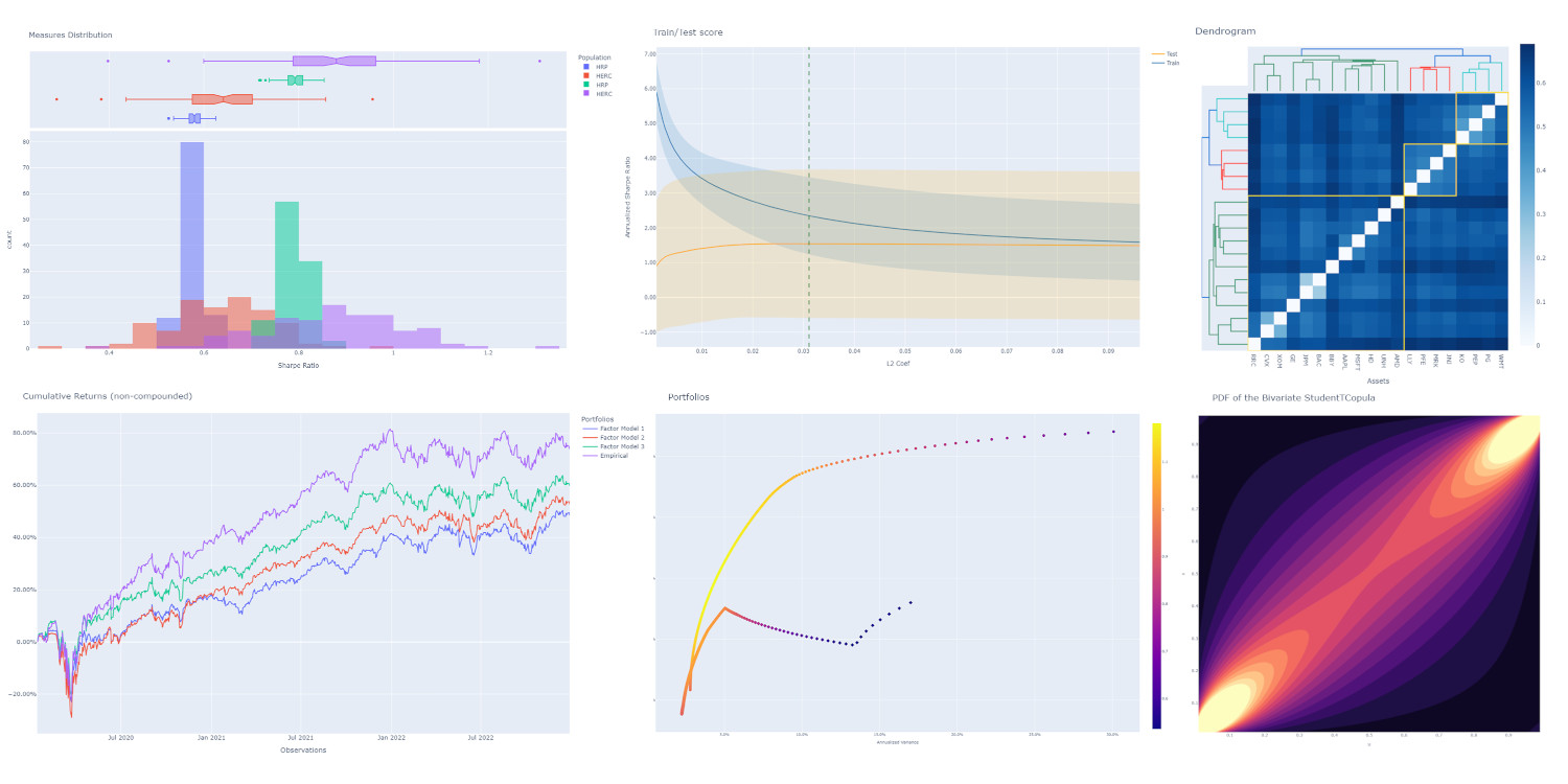
# index.html.md # skfolio **skfolio** is a Python library for portfolio optimization, factor model construction, and risk management built on top of scikit-learn. It offers a unified interface and tools compatible with scikit-learn to build, fine-tune, cross-validate, and stress-test portfolio models. It is distributed under the open-source 3-Clause BSD license. **skfolio** is backed by [Skfolio Labs](https://skfoliolabs.com), which provides enterprise support and SLAs for institutions. Portfolio optimization examples gallery from skfolio ## Important links - [Examples](https://skfolio.org/auto_examples/index.html) - [User Guide](https://skfolio.org/user_guide/index.html) - [API Reference](https://skfolio.org/api.html) - [GitHub Repo](https://github.com/skfolio/skfolio) - [Enterprise Support](https://skfoliolabs.com) ## Featured in * [Portfolio Optimization: Theory and Application](https://portfoliooptimizationbook.com/) by Daniel P. Palomar, includes Python code examples using skfolio. ## Installation `skfolio` requires Python 3.10 or later and can be installed with: ```bash pip install -U skfolio ``` See the [installation guide](https://skfolio.org/user_guide/install.html) for the full dependency list, for conda-forge and for the mixed-integer solvers. ## LLM-friendly documentation The documentation follows the [llms.txt convention](https://llmstxt.org/) and provides token-efficient Markdown alongside the HTML site: - Start with [llms.txt](https://skfolio.org/llms.txt) to find relevant pages. - Read only the Markdown pages needed by appending `.md` to their HTML URLs, for example [factor_models.html.md](https://skfolio.org/user_guide/factor_models.html.md). - Use [llms-full.txt](https://skfolio.org/llms-full.txt) only when the complete documentation is required in a single file. ## Contribution We welcome contributions of all kinds. Whether it’s reporting a bug, suggesting an improvement, or submitting code, your input helps make `skfolio` better. See the [contributing guide](https://github.com/skfolio/skfolio/blob/main/CONTRIBUTING.md) to get started. ## Key Concepts Since the development of modern portfolio theory by Markowitz (1952), mean-variance optimization (MVO) has received considerable attention. Unfortunately, it faces a number of shortcomings, including high sensitivity to the input parameters (expected returns and covariance), weight concentration, high turnover, and poor out-of-sample performance. It is well-known that naive allocation (1/N, inverse-vol, etc.) tends to outperform MVO out-of-sample (DeMiguel, 2007). Numerous approaches have been developed to alleviate these shortcomings (shrinkage, additional constraints, regularization, uncertainty set, higher moments, Bayesian approaches, coherent risk measures, left-tail risk optimization, distributionally robust optimization, factor model, risk-parity, hierarchical clustering, ensemble methods, pre-selection, etc.). Given the large number of methods, and the fact that they can be combined, there is a need for a unified framework with a machine-learning approach to perform model selection, validation, and parameter tuning while mitigating the risk of data leakage and overfitting. This framework is built on scikit-learn’s API. ## Available models * Portfolio Optimization: : * Naive: : * Equal-Weighted * Inverse-Volatility * Random (Dirichlet) * Convex: : * Mean-Risk * Risk Budgeting * Maximum Diversification * Distributionally Robust CVaR * Benchmark Tracker * Clustering: : * Hierarchical Risk Parity * Hierarchical Equal Risk Contribution * Schur Complementary Allocation * Nested Clusters Optimization * Ensemble Methods: : * Stacking Optimization * Prior Estimator: : * Empirical * Characteristics-Based Cross-Sectional Factor Model: : * 46 descriptors across 17 families (e.g. value, size, momentum, profitability) * Factor Exposures * Cross-Sectional Regression * Alpha Estimators * Forecast Evaluation * Ex-post and Ex-ante Attribution * Time-Series Factor Model * Black & Litterman * Synthetic Data (Stress Test, Factor Stress Test) * Entropy Pooling * Opinion Pooling * Expected Returns Estimator: : * Empirical * Exponentially Weighted * Equilibrium * Shrinkage * Covariance Estimator: : * Empirical * Gerber * Denoising * Detoning * Exponentially Weighted * Regime-Adjusted Exponentially Weighted * Ledoit-Wolf * Oracle Approximating Shrinkage * Shrunk Covariance * Graphical Lasso CV * Implied Covariance * Variance Estimator: : * Empirical * Exponentially Weighted * Regime-Adjusted Exponentially Weighted * Distance Estimator: : * Pearson Distance * Kendall Distance * Spearman Distance * Covariance Distance (based on any of the above covariance estimators) * Distance Correlation * Variation of Information * Distribution Estimator: : * Univariate: : * Gaussian * Student’s t * Johnson Su * Normal Inverse Gaussian * Bivariate Copula : * Gaussian Copula * Student’s t Copula * Clayton Copula * Gumbel Copula * Joe Copula * Independent Copula * Multivariate : * Vine Copula (Regular, Centered, Clustered, Conditional Sampling) * Uncertainty Set Estimator: : * On Expected Returns: : * Empirical * Circular Bootstrap * On Covariance: : * Empirical * Circular Bootstrap * Pre-Selection Transformers: : * Non-Dominated Selection * Select K Extremes (Best or Worst) * Drop Highly Correlated Assets * Select Non-Expiring Assets * Select Complete Assets (handle late inception, delisting, etc.) * Drop Zero Variance * Cross-Sectional Transformers: : * Standard Scaler (z-score) * Percentile Rank Scaler * Gaussian Rank Scaler (rank gaussianization) * Winsorizer (percentile clipping) * Tanh Shrinker (smooth outlier shrinkage) * Cross-Validation and Model Selection: : * Compatible with all `sklearn` methods (KFold, etc.) * Walk Forward * Combinatorial Purged Cross-Validation * Multiple Randomized Cross-Validation * Covariance Forecast Evaluation * Online Predict and Online Score * Hyper-Parameter Tuning: : * Compatible with all `sklearn` methods (GridSearchCV, RandomizedSearchCV) * Online Grid Search and Online Randomized Search * Risk Measures: : * Variance * Semi-Variance * Mean Absolute Deviation * First Lower Partial Moment * CVaR (Conditional Value at Risk) * EVaR (Entropic Value at Risk) * Worst Realization * CDaR (Conditional Drawdown at Risk) * Maximum Drawdown * Average Drawdown * EDaR (Entropic Drawdown at Risk) * Ulcer Index * Gini Mean Difference * Value at Risk * Drawdown at Risk * Entropic Risk Measure * Fourth Central Moment * Fourth Lower Partial Moment * Skew * Kurtosis * Optimization Features: : * Minimize Risk * Maximize Returns * Maximize Utility * Maximize Ratio * Transaction Costs * Management Fees * L1 and L2 Regularization * Weight Constraints * Group Constraints * Budget Constraints * Tracking Error Constraints * Turnover Constraints * Cardinality and Group Cardinality Constraints * Threshold (Long and Short) Constraints ## Quickstart The code snippets below are designed to introduce the functionality of `skfolio` so you can start using it quickly. It follows the same API as scikit-learn. ### Imports ```python from sklearn import set_config from sklearn.model_selection import ( GridSearchCV, KFold, RandomizedSearchCV, train_test_split, ) from sklearn.pipeline import Pipeline from scipy.stats import loguniform from skfolio import RatioMeasure, RiskMeasure from skfolio.datasets import ( load_factors_dataset, load_sp500_dataset, make_synthetic_characteristics, ) from skfolio.descriptor import ( BookToPrice, CashFlowToPrice, EWMarketBeta, EWMomentum, EWResidualVolatility, EWVolatility, LogMarketCap, SalesToPrice, ) from skfolio.distribution import VineCopula from skfolio.factor_exposure import ( DerivedFactor, FixedWeightedFactor, GlobalFactor, OneHotCategoricalFactors, ) from skfolio.model_selection import ( CombinatorialPurgedCV, WalkForward, cross_val_predict, ) from skfolio.moments import ( DenoiseCovariance, DetoneCovariance, EWMu, GerberCovariance, ShrunkMu, ) from skfolio.optimization import ( MeanRisk, HierarchicalRiskParity, NestedClustersOptimization, ObjectiveFunction, RiskBudgeting, ) from skfolio.pre_selection import SelectKExtremes from skfolio.preprocessing import prices_to_returns from skfolio.prior import ( BlackLitterman, CharacteristicsFactorModel, EmpiricalPrior, EntropyPooling, TimeSeriesFactorModel, OpinionPooling, SyntheticData, ) from skfolio.uncertainty_set import BootstrapMuUncertaintySet ``` ### Load Dataset ```python prices = load_sp500_dataset() ``` ### Train/Test split ```python X = prices_to_returns(prices) X_train, X_test = train_test_split(X, test_size=0.33, shuffle=False) ``` ### Minimum Variance ```python model = MeanRisk() ``` ### Fit on Training Set ```python model.fit(X_train) print(model.weights_) ``` ### Predict on Test Set ```python portfolio = model.predict(X_test) print(portfolio.annualized_sharpe_ratio) print(portfolio.summary()) ``` ### Maximum Sortino Ratio ```python model = MeanRisk( objective_function=ObjectiveFunction.MAXIMIZE_RATIO, risk_measure=RiskMeasure.SEMI_VARIANCE, ) ``` ### Denoised Covariance & Shrunk Expected Returns ```python model = MeanRisk( objective_function=ObjectiveFunction.MAXIMIZE_RATIO, prior_estimator=EmpiricalPrior( mu_estimator=ShrunkMu(), covariance_estimator=DenoiseCovariance() ), ) ``` ### Uncertainty Set on Expected Returns ```python model = MeanRisk( objective_function=ObjectiveFunction.MAXIMIZE_RATIO, mu_uncertainty_set_estimator=BootstrapMuUncertaintySet(), ) ``` ### Weight Constraints & Transaction Costs ```python model = MeanRisk( min_weights={"AAPL": 0.10, "JPM": 0.05}, max_weights=0.8, transaction_costs={"AAPL": 0.0001, "RRC": 0.0002}, groups=[ ["Equity"] * 3 + ["Fund"] * 5 + ["Bond"] * 12, ["US"] * 2 + ["Europe"] * 8 + ["Japan"] * 10, ], linear_constraints=[ "Equity <= 0.5 * Bond", "US >= 0.1", "Europe >= 0.5 * Fund", "Japan <= 1", ], ) model.fit(X_train) ``` ### Risk Parity on CVaR ```python model = RiskBudgeting(risk_measure=RiskMeasure.CVAR) ``` ### Risk Parity & Gerber Covariance ```python model = RiskBudgeting( prior_estimator=EmpiricalPrior(covariance_estimator=GerberCovariance()) ) ``` ### Nested Cluster Optimization with Cross-Validation and Parallelization ```python model = NestedClustersOptimization( inner_estimator=MeanRisk(risk_measure=RiskMeasure.CVAR), outer_estimator=RiskBudgeting(risk_measure=RiskMeasure.VARIANCE), cv=KFold(), n_jobs=-1, ) ``` ### Randomized Search of the L2 Norm ```python randomized_search = RandomizedSearchCV( estimator=MeanRisk(), cv=WalkForward(train_size=252, test_size=60), param_distributions={ "l2_coef": loguniform(1e-3, 1e-1), }, ) randomized_search.fit(X_train) best_model = randomized_search.best_estimator_ print(best_model.weights_) ``` ### Grid Search on Embedded Parameters ```python model = MeanRisk( objective_function=ObjectiveFunction.MAXIMIZE_RATIO, risk_measure=RiskMeasure.VARIANCE, prior_estimator=EmpiricalPrior(mu_estimator=EWMu(half_life=40)), ) print(model.get_params(deep=True)) gs = GridSearchCV( estimator=model, cv=KFold(n_splits=5, shuffle=False), n_jobs=-1, param_grid={ "risk_measure": [ RiskMeasure.VARIANCE, RiskMeasure.CVAR, RiskMeasure.CDAR, ], "prior_estimator__mu_estimator__half_life": [10, 20, 30, 40], }, ) gs.fit(X) best_model = gs.best_estimator_ print(best_model.weights_) ``` ### Black & Litterman Model ```python views = ["AAPL - BBY == 0.03 ", "CVX - KO == 0.04", "MSFT == 0.06 "] model = MeanRisk( objective_function=ObjectiveFunction.MAXIMIZE_RATIO, prior_estimator=BlackLitterman(views=views), ) ``` ### Characteristics-Based Factor Model ```python month = 21 quarter = 3 * month half_year = 6 * month year = 12 * month characteristics = make_synthetic_characteristics( n_assets=500, n_observations=2000, random_state=0, ) # Global factor market_factor = GlobalFactor(family="market") # Industry factors industry_factors = OneHotCategoricalFactors( category="industry", family="industry", ) # Style factors beta_factor = FixedWeightedFactor( descriptors=[ ("market_beta", EWMarketBeta(half_life=year)), ], transform_by_group="industry", ) momentum_factor = FixedWeightedFactor( descriptors=[ ("momentum", EWMomentum(half_life=half_year, skip=month)), ], transform_by_group="industry", ) size_factor = FixedWeightedFactor( descriptors=[("log_market_cap", LogMarketCap())], transform_by_group="industry", ) non_linear_size_factor = DerivedFactor( source="size", func=lambda x: x**3, transform_by_group="industry", ) value_factor = FixedWeightedFactor( descriptors=[ ("book_to_price", BookToPrice()), ("sales_to_price", SalesToPrice()), ("cash_flow_to_price", CashFlowToPrice()), ], weights=[0.8, 0.1, 0.1], transform_by_group="industry", ) volatility_factor = FixedWeightedFactor( descriptors=[ ("vol", EWVolatility(half_life=quarter)), ( "residual_vol", EWResidualVolatility( half_life=quarter, beta_half_life=quarter, ), ), ], transform_by_group="industry", ) # Characteristics factor model model = CharacteristicsFactorModel( factors=[ ("market", market_factor), ("industry", industry_factors), ("beta", beta_factor), ("momentum", momentum_factor), ("size", size_factor), ("non_linear_size", non_linear_size_factor), ("value", value_factor), ("volatility", volatility_factor), ], neutralize_against={ "volatility": ["beta"], "non_linear_size": ["size"], }, constrained_families=[("industry", None)], exposure_lag=1, inv_idio_variance_weight_shrinkage=0.5, n_jobs=-1, ) model.fit(characteristics=characteristics) factor_model = model.factor_model_ print(factor_model.summary()) ``` For complete workflows, see the [Factor Models user guide](https://skfolio.org/user_guide/factor_models.html) and the [Factor Models tutorials](https://skfolio.org/auto_examples/factor_models/index.html). ### Time-Series Factor Model ```python factor_prices = load_factors_dataset() X, factors = prices_to_returns(prices, factor_prices) X_train, X_test, factors_train, factors_test = train_test_split( X, factors, test_size=0.33, shuffle=False ) model = MeanRisk(prior_estimator=TimeSeriesFactorModel()) model.fit(X_train, factors=factors_train) print(model.weights_) portfolio = model.predict(X_test) print(portfolio.calmar_ratio) print(portfolio.summary()) ``` ### Time-Series Factor Model & Covariance Detoning ```python model = MeanRisk( prior_estimator=TimeSeriesFactorModel( factor_prior_estimator=EmpiricalPrior(covariance_estimator=DetoneCovariance()) ) ) ``` ### Black & Litterman Time-Series Factor Model ```python factor_views = ["MTUM - QUAL == 0.03 ", "VLUE == 0.06"] model = MeanRisk( objective_function=ObjectiveFunction.MAXIMIZE_RATIO, prior_estimator=TimeSeriesFactorModel( factor_prior_estimator=BlackLitterman(views=factor_views), ), ) ``` ### Pre-Selection Pipeline ```python set_config(transform_output="pandas") model = Pipeline( [ ("pre_selection", SelectKExtremes(k=10, highest=True)), ("optimization", MeanRisk()), ] ) model.fit(X_train) portfolio = model.predict(X_test) ``` ### K-fold Cross-Validation ```python model = MeanRisk() mpp = cross_val_predict(model, X_test, cv=KFold(n_splits=5)) # mpp is the predicted MultiPeriodPortfolio object composed of 5 Portfolios (1 per testing fold) mpp.plot_cumulative_returns() print(mpp.summary()) ``` ### Combinatorial Purged Cross-Validation ```python model = MeanRisk() cv = CombinatorialPurgedCV(n_folds=10, n_test_folds=2) print(cv.summary(X_train)) population = cross_val_predict(model, X_train, cv=cv) population.plot_distribution( measure_list=[RatioMeasure.SHARPE_RATIO, RatioMeasure.SORTINO_RATIO] ) population.plot_cumulative_returns() print(population.summary()) ``` ### Minimum CVaR Optimization on Synthetic Returns ```python vine = VineCopula(log_transform=True, n_jobs=-1) prior = SyntheticData(distribution_estimator=vine, n_samples=2000) model = MeanRisk(risk_measure=RiskMeasure.CVAR, prior_estimator=prior) model.fit(X) print(model.weights_) ``` ### Stress Test ```python vine = VineCopula(log_transform=True, central_assets=["BAC"], n_jobs=-1) vine.fit(X) X_stressed = vine.sample(n_samples=10_000, conditioning = {"BAC": -0.2}) ptf_stressed = model.predict(X_stressed) ``` ### Minimum CVaR Optimization on Synthetic Factors ```python vine = VineCopula(central_assets=["QUAL"], log_transform=True, n_jobs=-1) factor_prior = SyntheticData( distribution_estimator=vine, n_samples=10_000, sample_args=dict(conditioning={"QUAL": -0.2}), ) factor_model = TimeSeriesFactorModel(factor_prior_estimator=factor_prior) model = MeanRisk(risk_measure=RiskMeasure.CVAR, prior_estimator=factor_model) model.fit(X, factors=factors) print(model.weights_) ``` ### Factor Stress Test ```python factor_model.set_params(factor_prior_estimator__sample_args=dict( conditioning={"QUAL": -0.5} )) factor_model.fit(X, factors=factors) stressed_dist = factor_model.return_distribution_ stressed_ptf = model.predict(stressed_dist) ``` ### Entropy Pooling ```python entropy_pooling = EntropyPooling( mean_views=[ "JPM == -0.002", "PG >= LLY", "BAC >= prior(BAC) * 1.2", ], cvar_views=[ "GE == 0.08", ], ) entropy_pooling.fit(X) print(entropy_pooling.relative_entropy_) print(entropy_pooling.effective_number_of_scenarios_) print(entropy_pooling.return_distribution_.sample_weight) ``` ### CVaR Hierarchical Risk Parity optimization on Entropy Pooling ```python entropy_pooling = EntropyPooling(cvar_views=["GE == 0.08"]) model = HierarchicalRiskParity( risk_measure=RiskMeasure.CVAR, prior_estimator=entropy_pooling ) model.fit(X) print(model.weights_) ``` ### Stress Test with Entropy Pooling on Factor Synthetic Data ```python # Regular Vine Copula and sampling of 100,000 synthetic factor returns factor_synth = SyntheticData( n_samples=100_000, distribution_estimator=VineCopula(log_transform=True, n_jobs=-1, random_state=0) ) # Entropy Pooling by imposing a CVaR-95% of 10% on the Quality factor factor_entropy_pooling = EntropyPooling( prior_estimator=factor_synth, cvar_views=["QUAL == 0.10"], ) factor_model = TimeSeriesFactorModel(factor_prior_estimator=factor_entropy_pooling) factor_model.fit(X, factors=factors) # We retrieve the stressed distribution: stressed_dist = factor_model.return_distribution_ # We stress-test our portfolio: stressed_ptf = model.predict(stressed_dist) ``` ### Opinion Pooling ```python # We consider two expert opinions, each generated via Entropy Pooling with # user-defined views. # We assign probabilities of 40% to Expert 1, 50% to Expert 2, and by default # the remaining 10% is allocated to the prior distribution: opinion_1 = EntropyPooling(cvar_views=["AMD == 0.10"]) opinion_2 = EntropyPooling( mean_views=["AMD >= BAC", "JPM <= prior(JPM) * 0.8"], cvar_views=["GE == 0.12"], ) opinion_pooling = OpinionPooling( estimators=[("opinion_1", opinion_1), ("opinion_2", opinion_2)], opinion_probabilities=[0.4, 0.5], ) opinion_pooling.fit(X) ``` ## Docker You can also spin up a reproducible JupyterLab environment using Docker: Build the image: ```default docker build -t skfolio-jupyterlab . ``` Run the container: ```default docker run -p 8888:8888 -v :/app/data -it skfolio-jupyterlab ``` Browse: Open `localhost:8888/lab` and start using `skfolio` ## Recognition We would like to thank all contributors to our direct dependencies, such as [scikit-learn](https://github.com/scikit-learn/scikit-learn) and [cvxpy](https://github.com/cvxpy/cvxpy), as well as the contributors of the following resources: > * PyPortfolioOpt > * Riskfolio-Lib > * scikit-portfolio > * statsmodels > * rsome > * [Microprediction](https://github.com/microprediction) (Peter Cotton) > * [Portfolio Optimization Book](https://portfoliooptimizationbook.com/) (Daniel P. Palomar) > * *The Elements of Quantitative Investing* (Giuseppe Paleologo) > * [quantresearch.org](https://quantresearch.org) (Marcos López de Prado) > * gautier.marti.ai (Gautier Marti) ## Citation If you use `skfolio` in a scientific publication, we would appreciate citations: **The library:** ```bibtex @software{skfolio, title = {skfolio}, author = {Delatte, Hugo and Nicolini, Carlo and Manzi, Matteo}, version = {1.0.0}, year = {2026}, doi = {10.5281/zenodo.16148630}, url = {https://doi.org/10.5281/zenodo.16148630} } ``` The above uses the concept DOI, which always resolves to the latest release. If you need precise reproducibility, especially for journals or conferences that require it, you can cite the version-specific DOI for the exact release you used. To find it, go to our [Zenodo project page](https://doi.org/10.5281/zenodo.16148630), locate the release you wish to reference (e.g. “v1.0.0”), and copy the DOI listed next to that version. **The paper:** ```bibtex @article{nicolini2025skfolio, title = {skfolio: Portfolio Optimization in Python}, author = {Nicolini, Carlo and Manzi, Matteo and Delatte, Hugo}, journal = {arXiv preprint arXiv:2507.04176}, year = {2025}, eprint = {2507.04176}, archivePrefix = {arXiv}, url = {https://arxiv.org/abs/2507.04176} } ``` # _static/factor_model/fragments/alpha_eval_cumulative_ic.inc.html.md
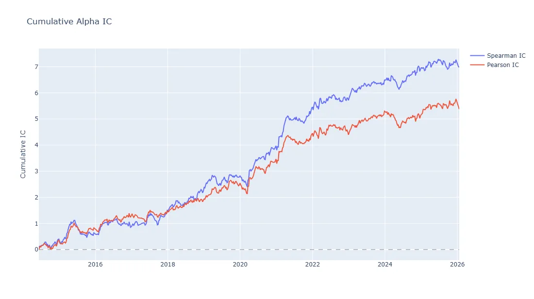
Cumulative Pearson and Spearman information coefficients for the alpha forecast over time
# _static/factor_model/fragments/alpha_eval_cumulative_returns.inc.html.md
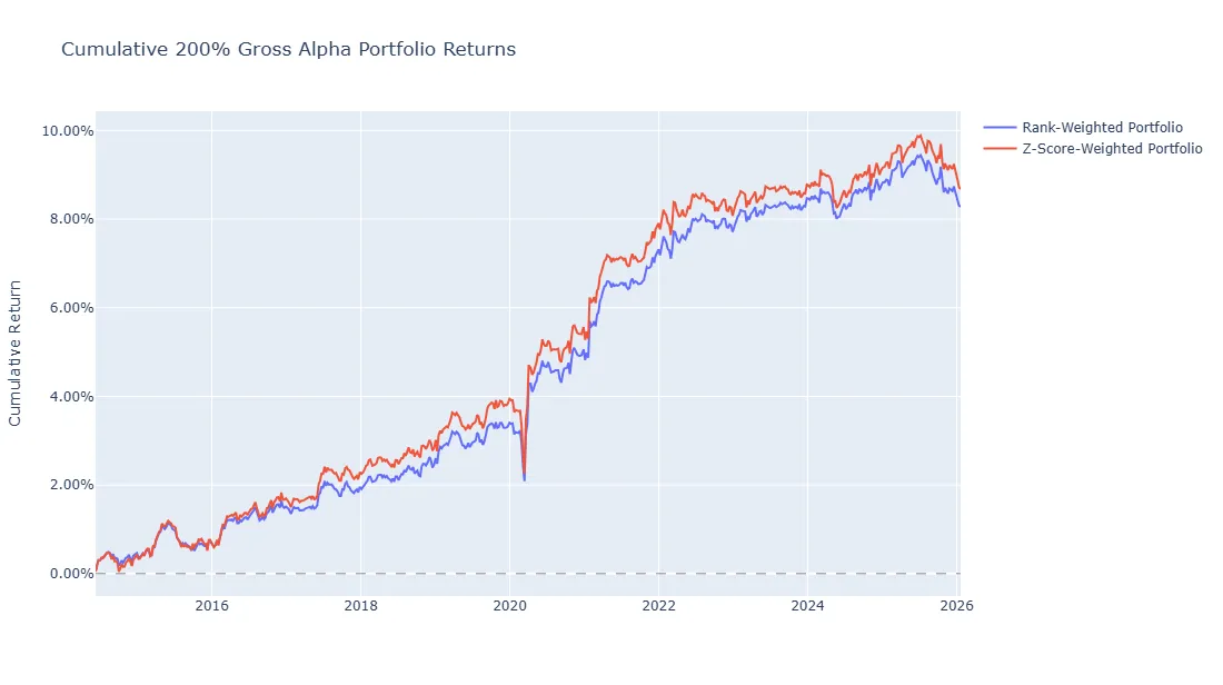
Cumulative returns of alpha-sorted long-short portfolios across holding periods
# _static/factor_model/fragments/alpha_eval_factor_correlation.inc.html.md
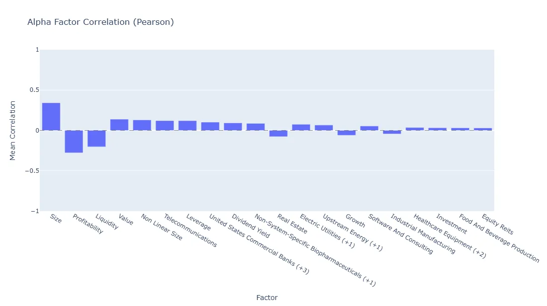
Correlation of the alpha forecast with market and style factor exposures
# _static/factor_model/fragments/alpha_realized_return_contrib.inc.html.md
Annualized realized return contributions of factors and the idiosyncratic component for the factor-neutral alpha portfolio
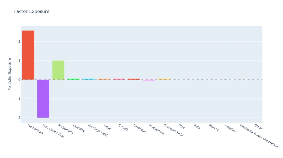
# _static/factor_model/fragments/attribution_predicted_exposure.inc.html.md
Factor exposures of the factor-constrained portfolio at the prediction date
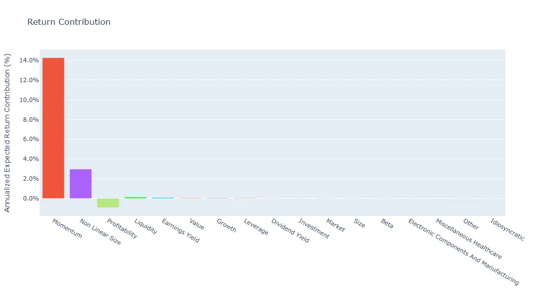
# _static/factor_model/fragments/attribution_predicted_return_contrib.inc.html.md
Predicted annualized return contributions by factor and idiosyncratic component
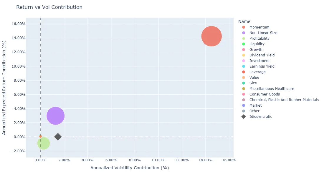
# _static/factor_model/fragments/attribution_predicted_return_vs_vol_contrib.inc.html.md
Predicted return contribution versus volatility contribution for each factor and the idiosyncratic component
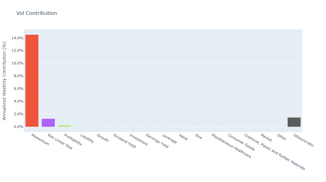
# _static/factor_model/fragments/attribution_predicted_vol_contrib.inc.html.md
Predicted annualized volatility contributions by factor and idiosyncratic component
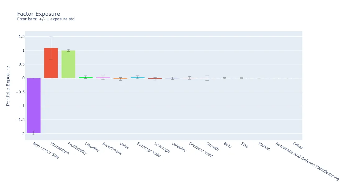
# _static/factor_model/fragments/attribution_realized_exposure.inc.html.md
Average realized factor exposures with one-standard-deviation error bars
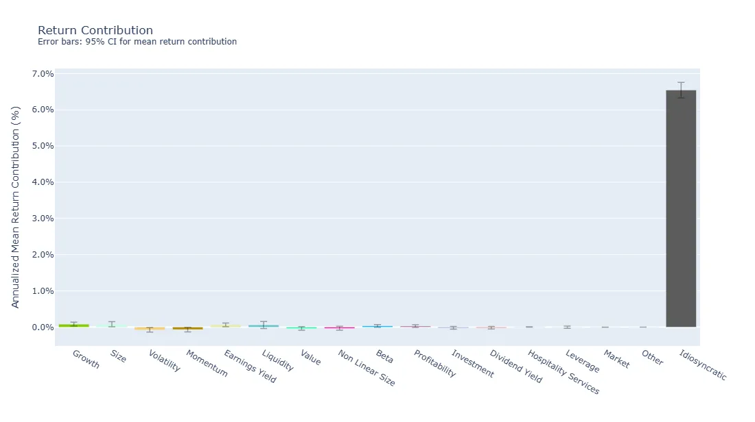
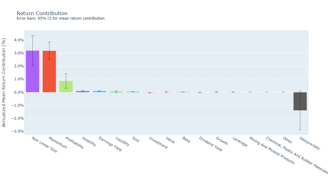
# _static/factor_model/fragments/attribution_realized_return_contrib.inc.html.md
Annualized realized return contributions by factor with 95% confidence intervals
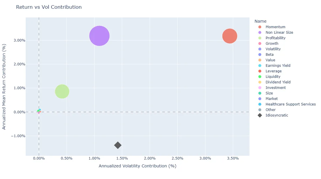
# _static/factor_model/fragments/attribution_realized_return_vs_vol_contrib.inc.html.md
Realized return contribution versus volatility contribution for each factor and the idiosyncratic component
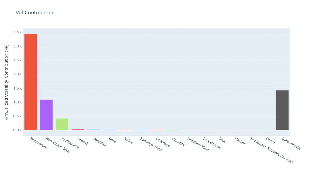
# _static/factor_model/fragments/attribution_realized_vol_contrib.inc.html.md
Realized annualized volatility contributions by factor and idiosyncratic component
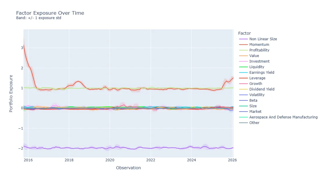
# _static/factor_model/fragments/attribution_rolling_realized_exposure.inc.html.md
Rolling factor exposures of the portfolio throughout the backtest
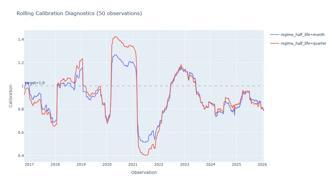
# _static/factor_model/fragments/covariance_cmp_calibration.inc.html.md
Rolling covariance forecast bias for models with one-month and one-quarter regime half-lives
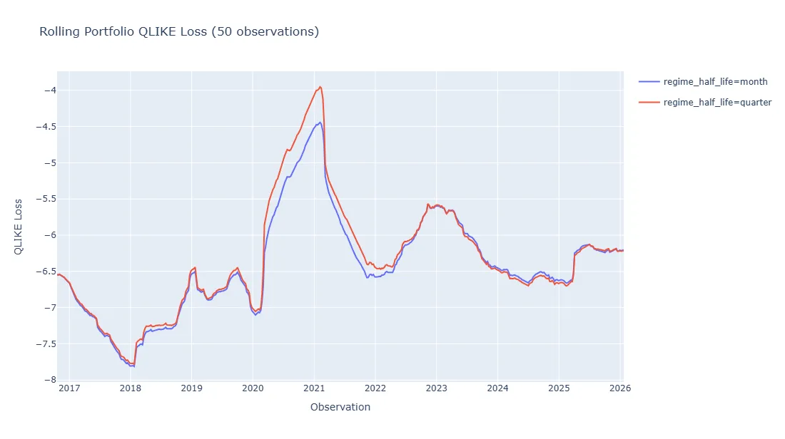
# _static/factor_model/fragments/covariance_cmp_qlike_loss.inc.html.md
Rolling QLIKE loss for covariance models with one-month and one-quarter regime half-lives
# _static/factor_model/fragments/covariance_eval_calibration.inc.html.md
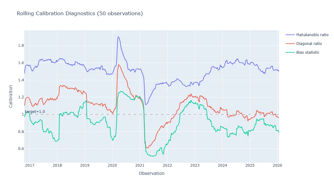
Rolling Mahalanobis, diagonal and portfolio bias calibration ratios for the covariance forecast
# _static/factor_model/fragments/factor_model_cs_regression_scores_adjusted_r2.inc.html.md
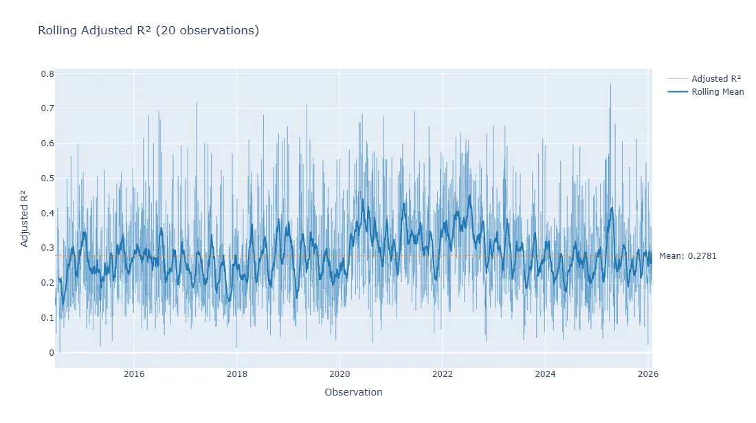
Rolling 20-day adjusted R-squared of the daily cross-sectional factor regressions
# _static/factor_model/fragments/factor_model_cs_regression_t_stat_exceedance_rate.inc.html.md
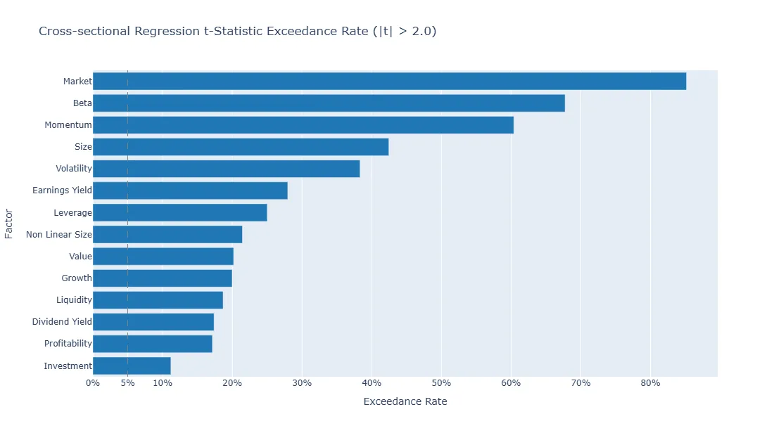
Share of dates on which each market or style factor return has an absolute t-statistic above two
# _static/factor_model/fragments/factor_model_cumulative_exposure_ic.inc.html.md
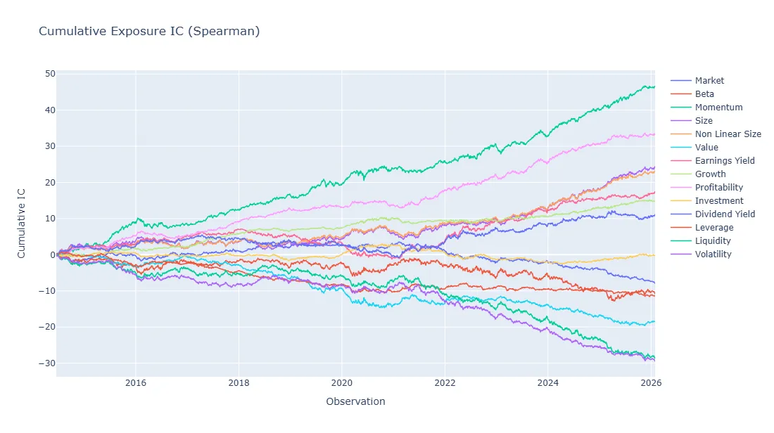
Cumulative information coefficients between factor exposures and next-period asset returns
# _static/factor_model/fragments/factor_model_exposure_correlation.inc.html.md
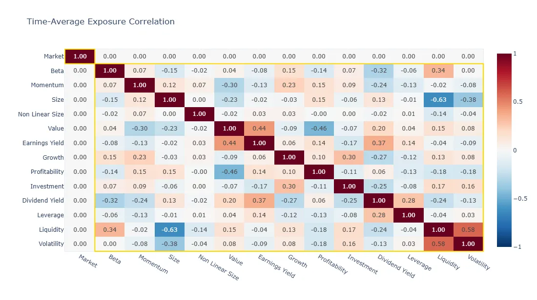
Time-average correlation heatmap for market and style factor exposures
# _static/factor_model/fragments/factor_model_exposure_stability.inc.html.md
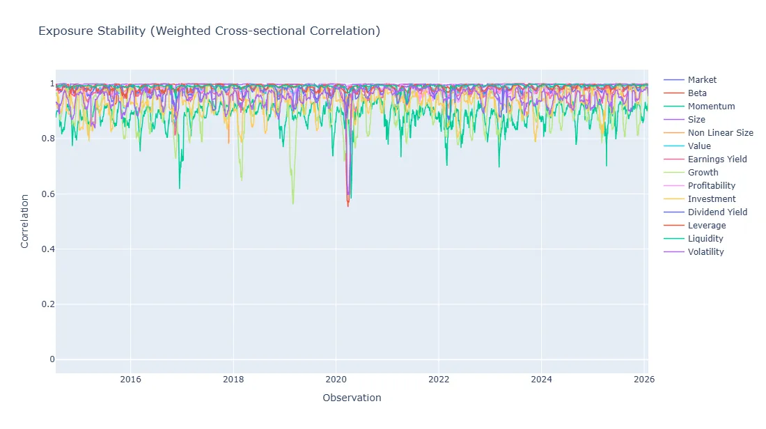
Monthly exposure stability through time for market and style factors
# _static/factor_model/fragments/factor_model_factor_cumulative_returns.inc.html.md
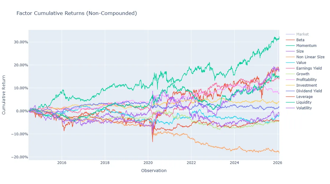
Cumulative realized returns through time for market and style factors
# _static/factor_model/fragments/factor_model_factor_forecast_correlation.inc.html.md
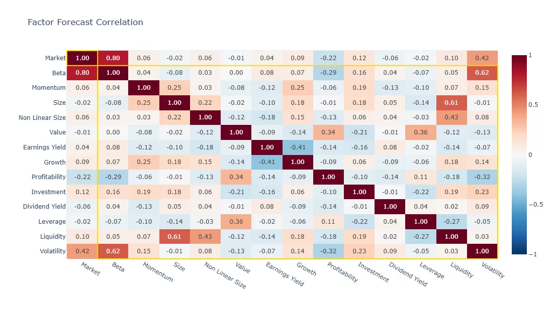
Forecast return correlation heatmap for market and style factors
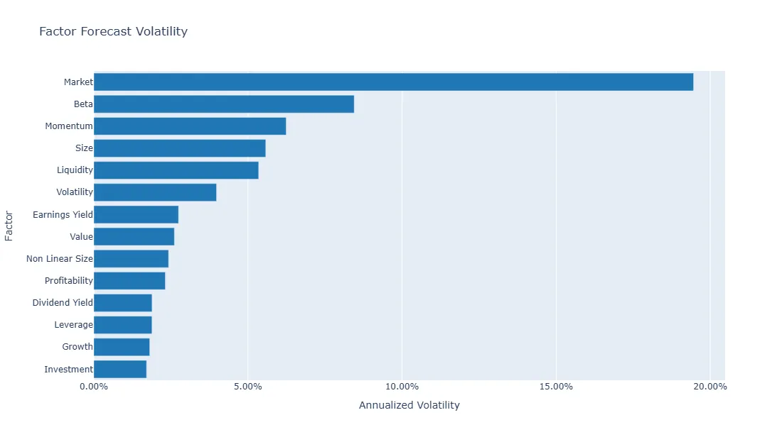
# _static/factor_model/fragments/factor_model_factor_forecast_volatilities.inc.html.md
Annualized forecast volatilities for market and style factors
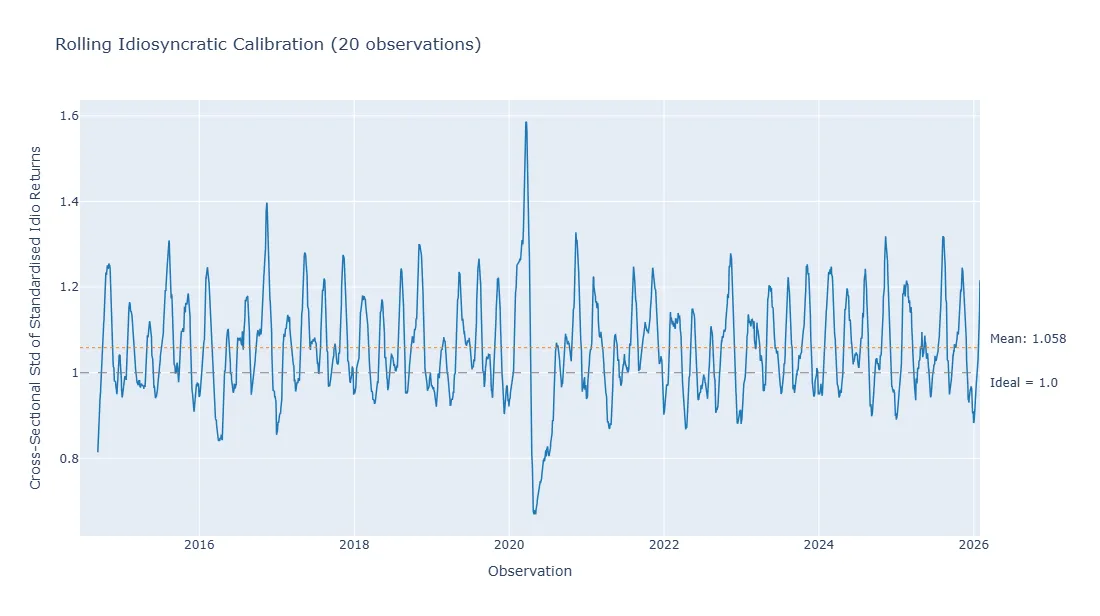
# _static/factor_model/fragments/factor_model_idio_calibration.inc.html.md
Rolling cross-sectional standard deviation of standardized idiosyncratic returns relative to the calibration target
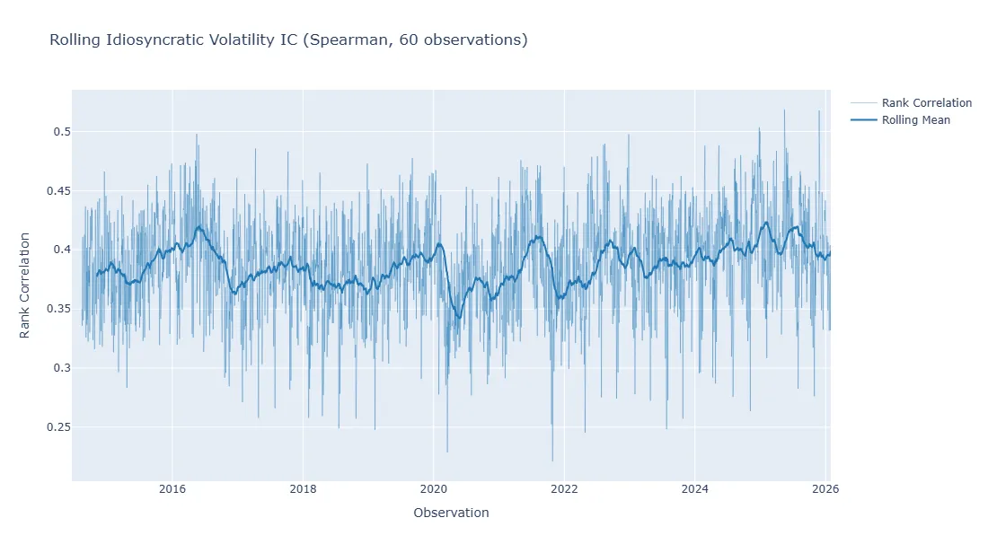
# _static/factor_model/fragments/factor_model_idio_vol_ic.inc.html.md
Information coefficient through time for predicted versus realized idiosyncratic volatility ranks
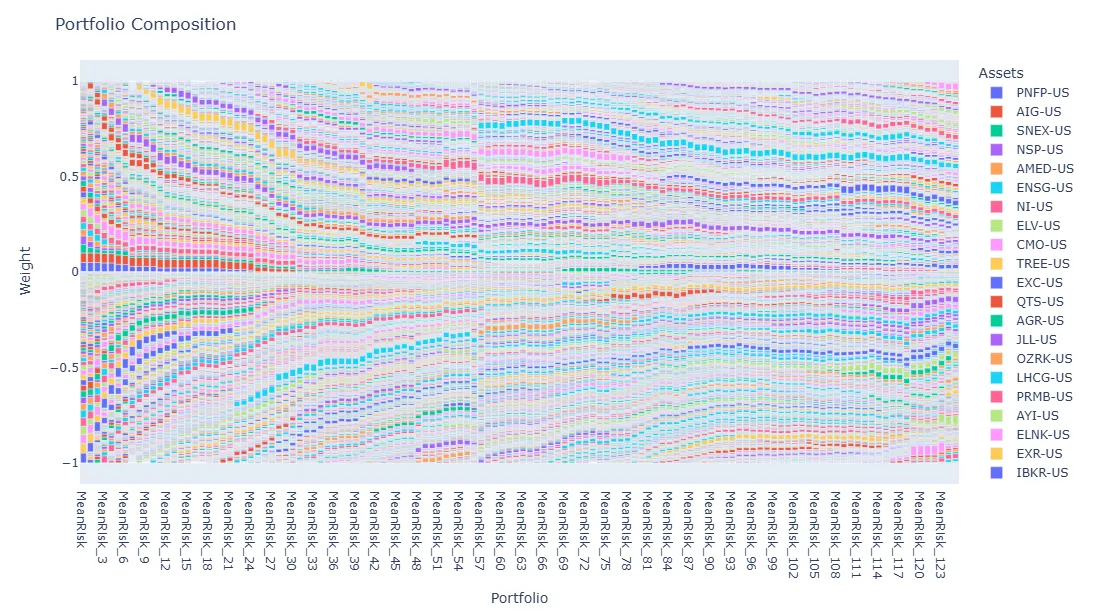
# _static/factor_model/fragments/mpp_composition.inc.html.md
Long and short asset weights of the factor-constrained portfolio across monthly rebalancing dates
# _static/factor_model/fragments/mpp_cumulative_returns.inc.html.md
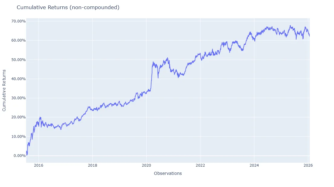
Cumulative out-of-sample return of the monthly rebalanced factor-constrained portfolio
# _static/factor_model/tables/alpha_eval_ic_summary.inc.html.md
mean std icir t_stat hit_rate
spearman_ic 0.012 0.073 0.164 3.965 0.556
pearson_ic 0.009 0.068 0.135 3.255 0.539
# _static/factor_model/tables/alpha_eval_portfolio_summary.inc.html.md
annualized_mean annualized_vol annualized_ir hit_rate mean_turnover
rank_weighted_portfolio 0.036 0.019 1.869 0.554 1.599
zscore_weighted_portfolio 0.037 0.022 1.710 0.552 1.745
# _static/factor_model/tables/attribution_predicted_factors_head.inc.html.md
Family Exposure Volatility Contribution % of Total Variance Expected Return Contribution Standalone Volatility Standalone Expected Return Correlation with Portfolio
Factor
momentum style 2.5762 14.51% 83.05% 14.25% 6.24% 5.53% 0.9025
non_linear_size style -2.0000 1.27% 7.29% 2.97% 2.42% -1.48% -0.2629
profitability style 1.0000 0.25% 1.46% -0.92% 2.32% -0.92% 0.1097
liquidity style 0.0500 -0.02% -0.10% 0.14% 5.35% 2.77% -0.0628
growth style 0.0500 0.02% 0.09% 0.05% 1.81% 0.96% 0.1813
# _static/factor_model/tables/attribution_predicted_families.inc.html.md
Exposure Volatility Contribution % of Total Variance Expected Return Contribution
Family
style 1.8262 16.00% 91.57% 16.69%
industry -0.0000 0.00% 0.00% 0.00%
market -0.0000 -0.00% -0.00% -0.00%
# _static/factor_model/tables/attribution_predicted_summary.inc.html.md
Volatility Contribution % of Total Variance Expected Return Contribution
Component
Systematic 16.00% 91.57% 16.69%
Idiosyncratic 1.47% 8.43% 0.00%
Total 17.47% 100.00% 16.69%
# _static/factor_model/tables/attribution_realized_factors_head.inc.html.md
Family Exposure Mean Exposure Std Volatility Contribution % of Total Variance Mean Return Contribution (95% CI) Standalone Volatility Standalone Mean Return Correlation with Portfolio
Factor
momentum style 1.0852 0.4029 3.44% 53.04% 3.18% ± 0.67% 4.60% 2.56% 0.6621
non_linear_size style -1.9746 0.0726 1.09% 16.81% 3.19% ± 1.16% 1.93% -1.63% -0.2880
profitability style 0.9970 0.0400 0.42% 6.45% 0.86% ± 0.56% 1.58% 0.83% 0.2665
growth style -0.0042 0.0827 0.04% 0.57% 0.01% ± 0.05% 1.65% -0.41% 0.1788
volatility style -0.0101 0.0436 0.02% 0.34% 0.09% ± 0.04% 3.31% -0.06% -0.2287
# _static/factor_model/tables/attribution_realized_families.inc.html.md
Exposure Mean Exposure Std Volatility Contribution % of Total Variance Mean Return Contribution (95% CI)
Family
style 0.1468 0.4464 5.07% 78.10% 7.51% ± 1.48%
industry 0.0004 0.0039 -0.00% -0.03% 0.00% ± 0.01%
market 0.0004 0.0039 0.00% 0.02% 0.00% ± 0.00%
# _static/factor_model/tables/attribution_realized_summary.inc.html.md
Volatility Contribution % of Total Variance Mean Return Contribution (95% CI)
Component
Systematic 5.07% 78.09% 7.51% ± 1.48%
Idiosyncratic 1.42% 21.93% -1.39% ± 1.48%
Unattributed -0.00% -0.02% -0.22%
Total 6.49% 100.00% 5.90%
# _static/factor_model/tables/attribution_rolling_realized_summary.inc.html.md
Volatility Contribution % of Total Variance Mean Return Contribution (95% CI)
Observation Component
2015-10-09 Systematic 6.05% 61.57% 34.24% ± 11.08%
Idiosyncratic 3.79% 38.54% 5.60% ± 11.08%
Unattributed -0.01% -0.11% -1.19%
Total 9.82% 100.00% 38.66%
2015-11-09 Systematic 7.12% 80.97% 30.77% ± 11.05%
Idiosyncratic 1.67% 19.04% 0.08% ± 11.05%
Unattributed -0.00% -0.00% -0.64%
Total 8.79% 100.00% 30.21%
# _static/factor_model/tables/covariance_comparison_summary.inc.html.md
estimator regime_half_life=month regime_half_life=quarter
mean median std p5 p95 mad_from_target target mean median std p5 p95 mad_from_target target
Mahalanobis ratio 1.505 1.320 0.789 0.672 2.969 0.606 1.000 1.504 1.310 0.792 0.672 2.974 0.604 1.000
Diagonal ratio 1.087 0.921 0.817 0.349 2.207 0.453 1.000 1.080 0.896 0.964 0.319 2.292 0.470 1.000
Portfolio standardized returns 0.096 0.140 0.917 -1.545 1.360 0.695 mean=0, std=1 0.086 0.133 0.937 -1.586 1.324 0.690 mean=0, std=1
Portfolio QLIKE -6.411 -6.696 1.700 -7.919 -4.387 lower is better -6.346 -6.694 2.024 -7.896 -4.426 lower is better
# _static/factor_model/tables/covariance_evaluation_summary.inc.html.md
mean median std p5 p95 mad_from_target target
Mahalanobis ratio 1.505 1.320 0.789 0.672 2.969 0.606 1.000
Diagonal ratio 1.087 0.921 0.817 0.349 2.207 0.453 1.000
Portfolio standardized returns 0.096 0.140 0.917 -1.545 1.360 0.695 mean=0, std=1
Portfolio QLIKE -6.411 -6.696 1.700 -7.919 -4.387 lower is better
# _static/factor_model/tables/factor_model_exposure_ic_summary.inc.html.md
mean_ic std_ic ic_ir hit_rate
market -0.003 0.095 -0.029 0.495
beta -0.004 0.169 -0.022 0.497
momentum 0.016 0.154 0.103 0.564
size 0.008 0.141 0.059 0.528
non_linear_size 0.008 0.124 0.063 0.532
value -0.006 0.111 -0.057 0.459
earnings_yield 0.006 0.119 0.051 0.509
growth 0.005 0.068 0.075 0.548
profitability 0.011 0.098 0.117 0.552
investment -0.000 0.067 -0.001 0.495
dividend_yield 0.004 0.125 0.031 0.505
leverage -0.004 0.075 -0.052 0.475
liquidity -0.010 0.155 -0.064 0.475
volatility -0.010 0.132 -0.076 0.464
# _static/factor_model/tables/style_factor_summary.inc.html.md
annualized_mean annualized_vol annualized_sharpe mean_vif
beta 0.015 0.056 0.265 1.530
momentum 0.028 0.044 0.622 1.461
size 0.016 0.041 0.385 3.658
non_linear_size -0.016 0.019 -0.833 1.518
value -0.001 0.019 -0.072 2.324
earnings_yield 0.012 0.023 0.530 1.958
growth -0.004 0.016 -0.228 1.330
profitability 0.007 0.015 0.443 1.814
investment 0.003 0.011 0.294 1.256
dividend_yield 0.002 0.015 0.114 1.518
leverage -0.004 0.016 -0.225 1.248
liquidity 0.012 0.032 0.379 4.587
volatility -0.001 0.032 -0.046 1.900
# api.html.md # API Reference This is the class and function reference of `skfolio`. Please refer to the [full user guide](https://skfolio.org/user_guide/index.html.md#user-guide) for further details, as the class and function raw specifications may not be enough to give full guidelines on their uses. ## [`skfolio.measures`](https://skfolio.org/api.html.md#module-skfolio.measures): Measures Module that includes all Measures functions used across `skfolio`. ### Base Class | [`measures.BaseMeasure`](https://skfolio.org/generated/skfolio.measures.BaseMeasure.html.md#skfolio.measures.BaseMeasure) | Base Enum of measures. | |------------------------------------------------------------------------------------------------------|--------------------------| ### Classes | [`measures.PerfMeasure`](https://skfolio.org/generated/skfolio.measures.PerfMeasure.html.md#skfolio.measures.PerfMeasure) | Enumeration of performance measures. | |--------------------------------------------------------------------------------------------------------------|---------------------------------------------------------------------| | [`measures.RiskMeasure`](https://skfolio.org/generated/skfolio.measures.RiskMeasure.html.md#skfolio.measures.RiskMeasure) | Enumeration of risk measures. | | [`measures.ExtraRiskMeasure`](https://skfolio.org/generated/skfolio.measures.ExtraRiskMeasure.html.md#skfolio.measures.ExtraRiskMeasure) | Enumeration of other risk measures not used in convex optimization. | | [`measures.RatioMeasure`](https://skfolio.org/generated/skfolio.measures.RatioMeasure.html.md#skfolio.measures.RatioMeasure) | Enumeration of ratio measures. | ### Functions | [`measures.mean`](https://skfolio.org/generated/skfolio.measures.mean.html.md#skfolio.measures.mean)(returns[, sample_weight]) | Compute the mean. | |---------------------------------------------------------------------------------------------------------------------------------------------|-----------------------------------------------------------------------------------------| | [`measures.get_cumulative_returns`](https://skfolio.org/generated/skfolio.measures.get_cumulative_returns.html.md#skfolio.measures.get_cumulative_returns)(returns[, ...]) | Compute the cumulative returns from a series of returns. | | [`measures.get_drawdowns`](https://skfolio.org/generated/skfolio.measures.get_drawdowns.html.md#skfolio.measures.get_drawdowns)(returns[, compounded]) | Compute the drawdowns' series from the returns. | | [`measures.variance`](https://skfolio.org/generated/skfolio.measures.variance.html.md#skfolio.measures.variance)(returns[, biased, ...]) | Compute the variance (second moment). | | [`measures.semi_variance`](https://skfolio.org/generated/skfolio.measures.semi_variance.html.md#skfolio.measures.semi_variance)(returns[, ...]) | Compute the semi-variance (second lower partial moment). | | [`measures.standard_deviation`](https://skfolio.org/generated/skfolio.measures.standard_deviation.html.md#skfolio.measures.standard_deviation)(returns[, ...]) | Compute the standard-deviation (square root of the second moment). | | [`measures.semi_deviation`](https://skfolio.org/generated/skfolio.measures.semi_deviation.html.md#skfolio.measures.semi_deviation)(returns[, ...]) | Compute the semi-deviation (square root of the second lower partial moment). | | [`measures.third_central_moment`](https://skfolio.org/generated/skfolio.measures.third_central_moment.html.md#skfolio.measures.third_central_moment)(returns[, ...]) | Compute the third central moment. | | [`measures.fourth_central_moment`](https://skfolio.org/generated/skfolio.measures.fourth_central_moment.html.md#skfolio.measures.fourth_central_moment)(returns[, ...]) | Compute the Fourth central moment. | | [`measures.fourth_lower_partial_moment`](https://skfolio.org/generated/skfolio.measures.fourth_lower_partial_moment.html.md#skfolio.measures.fourth_lower_partial_moment)(returns) | Compute the fourth lower partial moment. | | [`measures.skew`](https://skfolio.org/generated/skfolio.measures.skew.html.md#skfolio.measures.skew)(returns[, sample_weight]) | Compute the Skew. | | [`measures.kurtosis`](https://skfolio.org/generated/skfolio.measures.kurtosis.html.md#skfolio.measures.kurtosis)(returns[, sample_weight]) | Compute the Kurtosis. | | [`measures.cvar`](https://skfolio.org/generated/skfolio.measures.cvar.html.md#skfolio.measures.cvar)(returns[, beta, sample_weight]) | Compute the historical CVaR (conditional value at risk). | | [`measures.mean_absolute_deviation`](https://skfolio.org/generated/skfolio.measures.mean_absolute_deviation.html.md#skfolio.measures.mean_absolute_deviation)(returns[, ...]) | Compute the mean absolute deviation (MAD). | | [`measures.value_at_risk`](https://skfolio.org/generated/skfolio.measures.value_at_risk.html.md#skfolio.measures.value_at_risk)(returns[, beta, ...]) | Compute the historical value at risk (VaR). | | [`measures.worst_realization`](https://skfolio.org/generated/skfolio.measures.worst_realization.html.md#skfolio.measures.worst_realization)(returns) | Compute the worst realization (worst return). | | [`measures.first_lower_partial_moment`](https://skfolio.org/generated/skfolio.measures.first_lower_partial_moment.html.md#skfolio.measures.first_lower_partial_moment)(returns) | Compute the first lower partial moment. | | [`measures.entropic_risk_measure`](https://skfolio.org/generated/skfolio.measures.entropic_risk_measure.html.md#skfolio.measures.entropic_risk_measure)(returns[, ...]) | Compute the entropic risk measure. | | [`measures.evar`](https://skfolio.org/generated/skfolio.measures.evar.html.md#skfolio.measures.evar)(returns[, beta]) | Compute the EVaR (entropic value at risk) and its associated risk aversion. | | [`measures.drawdown_at_risk`](https://skfolio.org/generated/skfolio.measures.drawdown_at_risk.html.md#skfolio.measures.drawdown_at_risk)(drawdowns[, beta]) | Compute the Drawdown at risk. | | [`measures.cdar`](https://skfolio.org/generated/skfolio.measures.cdar.html.md#skfolio.measures.cdar)(drawdowns[, beta]) | Compute the historical CDaR (conditional drawdown at risk). | | [`measures.max_drawdown`](https://skfolio.org/generated/skfolio.measures.max_drawdown.html.md#skfolio.measures.max_drawdown)(drawdowns) | Compute the maximum drawdown. | | [`measures.average_drawdown`](https://skfolio.org/generated/skfolio.measures.average_drawdown.html.md#skfolio.measures.average_drawdown)(drawdowns) | Compute the average drawdown. | | [`measures.edar`](https://skfolio.org/generated/skfolio.measures.edar.html.md#skfolio.measures.edar)(drawdowns[, beta]) | Compute the EDaR (entropic drawdown at risk). | | [`measures.ulcer_index`](https://skfolio.org/generated/skfolio.measures.ulcer_index.html.md#skfolio.measures.ulcer_index)(drawdowns) | Compute the Ulcer index. | | [`measures.gini_mean_difference`](https://skfolio.org/generated/skfolio.measures.gini_mean_difference.html.md#skfolio.measures.gini_mean_difference)(returns) | Compute the Gini mean difference (GMD). | | [`measures.owa_gmd_weights`](https://skfolio.org/generated/skfolio.measures.owa_gmd_weights.html.md#skfolio.measures.owa_gmd_weights)(n_observations) | Compute the OWA weights used for the Gini mean difference (GMD) computation. | | [`measures.effective_number_assets`](https://skfolio.org/generated/skfolio.measures.effective_number_assets.html.md#skfolio.measures.effective_number_assets)(weights) | Compute the effective number of assets, defined as the inverse of the Herfindahl index. | | [`measures.correlation`](https://skfolio.org/generated/skfolio.measures.correlation.html.md#skfolio.measures.correlation)(X[, sample_weight]) | Compute the correlation matrix. | ## [`skfolio.portfolio`](https://skfolio.org/api.html.md#module-skfolio.portfolio): Portfolio Portfolio module. `Portfolio` and `MultiPeriodPortfolio` objects are returned by the `predict` method of Optimization estimators. They must be consistent with the convex optimization problems, meaning that `Portfolio` is the dot product of the assets weights with the assets returns and `MultiPeriodPortfolio` is a list of `Portfolio`. ### Base Class | [`portfolio.BasePortfolio`](https://skfolio.org/generated/skfolio.portfolio.BasePortfolio.html.md#skfolio.portfolio.BasePortfolio) | Base Portfolio class for all portfolios in skfolio. | |------------------------------------------------------------------------------------------------------------|-------------------------------------------------------| ### Classes | [`portfolio.Portfolio`](https://skfolio.org/generated/skfolio.portfolio.Portfolio.html.md#skfolio.portfolio.Portfolio) | Portfolio class. | |------------------------------------------------------------------------------------------------------------------------|------------------------------------------------------------| | [`portfolio.FailedPortfolio`](https://skfolio.org/generated/skfolio.portfolio.FailedPortfolio.html.md#skfolio.portfolio.FailedPortfolio) | Portfolio object returned when an optimization step fails. | | [`portfolio.MultiPeriodPortfolio`](https://skfolio.org/generated/skfolio.portfolio.MultiPeriodPortfolio.html.md#skfolio.portfolio.MultiPeriodPortfolio) | Multi-Period Portfolio class. | ## [`skfolio.population`](https://skfolio.org/api.html.md#module-skfolio.population): Population Population module. ### Classes | [`population.Population`](https://skfolio.org/generated/skfolio.population.Population.html.md#skfolio.population.Population) | Population Class. | |--------------------------------------------------------------------------------------------------------|---------------------| ## [`skfolio.containers`](https://skfolio.org/api.html.md#module-skfolio.containers): Containers Containers module. ### Classes | [`containers.AssetPanel`](https://skfolio.org/generated/skfolio.containers.AssetPanel.html.md#skfolio.containers.AssetPanel) | Container for aligned cross-sectional asset data. | |--------------------------------------------------------------------------------------------------------------|-----------------------------------------------------| | [`containers.AssetPanelView`](https://skfolio.org/generated/skfolio.containers.AssetPanelView.html.md#skfolio.containers.AssetPanelView) | Observation-sliced view into an `AssetPanel`. | ### Field Base Class | [`containers.BaseField`](https://skfolio.org/generated/skfolio.containers.BaseField.html.md#skfolio.containers.BaseField) | Base class for fields stored in an `AssetPanel`. | |------------------------------------------------------------------------------------------------------------------|----------------------------------------------------------------| | [`containers.Field2D`](https://skfolio.org/generated/skfolio.containers.Field2D.html.md#skfolio.containers.Field2D) | Numeric 2D field with axes (observations, assets). | | [`containers.Field3D`](https://skfolio.org/generated/skfolio.containers.Field3D.html.md#skfolio.containers.Field3D) | Numeric 3D field with axes (observations, assets, third_axis). | | [`containers.FieldCategorical`](https://skfolio.org/generated/skfolio.containers.FieldCategorical.html.md#skfolio.containers.FieldCategorical) | Integer-coded categorical 2D field. | ### Enum | [`containers.InactivePolicy`](https://skfolio.org/generated/skfolio.containers.InactivePolicy.html.md#skfolio.containers.InactivePolicy) | Validation policy for values outside an `AssetPanel` active universe. | |----------------------------------------------------------------------------------------------------------------|-------------------------------------------------------------------------| ### Functions | [`containers.concat`](https://skfolio.org/generated/skfolio.containers.concat.html.md#skfolio.containers.concat)(panels, \*[, ...]) | Concatenate panels along the observation axis. | |-------------------------------------------------------------------------------------------------------------------|--------------------------------------------------| ## [`skfolio.base`](https://skfolio.org/api.html.md#module-skfolio.base): Base Estimators Base classes for all estimators and various utility functions. ### Classes | [`base.BaseAssetPanelTransformer`](https://skfolio.org/generated/skfolio.base.BaseAssetPanelTransformer.html.md#skfolio.base.BaseAssetPanelTransformer) | Base class for estimators that transform asset panel data. | |--------------------------------------------------------------------------------------------------------------------------|--------------------------------------------------------------| | [`base.BaseComposition`](https://skfolio.org/generated/skfolio.base.BaseComposition.html.md#skfolio.base.BaseComposition) | Handles parameter management for ensemble estimators. | ## `skfolio.optimization.base`: Base Optimization Estimator Optimization module. ### Classes | [`optimization.BaseOptimization`](https://skfolio.org/generated/skfolio.optimization.BaseOptimization.html.md#skfolio.optimization.BaseOptimization) | Base class for all portfolio optimizations in skfolio. | |------------------------------------------------------------------------------------------------------------------------|----------------------------------------------------------| ## [`skfolio.optimization.naive`](https://skfolio.org/api.html.md#module-skfolio.optimization.naive): Naive Optimization Estimators Naive Optimization module. ### Classes | [`optimization.EqualWeighted`](https://skfolio.org/generated/skfolio.optimization.EqualWeighted.html.md#skfolio.optimization.EqualWeighted) | Equally Weighted estimator. | |------------------------------------------------------------------------------------------------------------------------|-------------------------------| | [`optimization.InverseVolatility`](https://skfolio.org/generated/skfolio.optimization.InverseVolatility.html.md#skfolio.optimization.InverseVolatility) | Inverse Volatility estimator. | | [`optimization.Random`](https://skfolio.org/generated/skfolio.optimization.Random.html.md#skfolio.optimization.Random) | Random weight estimator. | ## [`skfolio.optimization.convex`](https://skfolio.org/api.html.md#module-skfolio.optimization.convex): Convex Optimization Estimators Convex Optimization module. ### Enum | [`optimization.ObjectiveFunction`](https://skfolio.org/generated/skfolio.optimization.ObjectiveFunction.html.md#skfolio.optimization.ObjectiveFunction) | Enumeration of objective functions. | |--------------------------------------------------------------------------------------------------------------------------|---------------------------------------| ### Classes | [`optimization.ConvexOptimization`](https://skfolio.org/generated/skfolio.optimization.ConvexOptimization.html.md#skfolio.optimization.ConvexOptimization) | Base class for all convex optimization estimators in skfolio. | |------------------------------------------------------------------------------------------------------------------------------------------|-----------------------------------------------------------------| | [`optimization.MeanRisk`](https://skfolio.org/generated/skfolio.optimization.MeanRisk.html.md#skfolio.optimization.MeanRisk) | Mean-Risk Optimization estimator. | | [`optimization.BenchmarkTracker`](https://skfolio.org/generated/skfolio.optimization.BenchmarkTracker.html.md#skfolio.optimization.BenchmarkTracker) | Benchmark Tracker Optimization estimator. | | [`optimization.RiskBudgeting`](https://skfolio.org/generated/skfolio.optimization.RiskBudgeting.html.md#skfolio.optimization.RiskBudgeting) | Risk Budgeting Optimization estimator. | | [`optimization.MaximumDiversification`](https://skfolio.org/generated/skfolio.optimization.MaximumDiversification.html.md#skfolio.optimization.MaximumDiversification) | Maximum Diversification Optimization estimator. | | [`optimization.DistributionallyRobustCVaR`](https://skfolio.org/generated/skfolio.optimization.DistributionallyRobustCVaR.html.md#skfolio.optimization.DistributionallyRobustCVaR) | Distributionally Robust CVaR. | ## [`skfolio.optimization.cluster`](https://skfolio.org/api.html.md#module-skfolio.optimization.cluster): Clustering Optimization Estimators Cluster Optimization module. ### Classes | [`optimization.BaseHierarchicalOptimization`](https://skfolio.org/generated/skfolio.optimization.BaseHierarchicalOptimization.html.md#skfolio.optimization.BaseHierarchicalOptimization) | Base Hierarchical Clustering Optimization estimator. | |--------------------------------------------------------------------------------------------------------------------------------------------------------|--------------------------------------------------------| | [`optimization.HierarchicalRiskParity`](https://skfolio.org/generated/skfolio.optimization.HierarchicalRiskParity.html.md#skfolio.optimization.HierarchicalRiskParity) | Hierarchical Risk Parity estimator. | | [`optimization.HierarchicalEqualRiskContribution`](https://skfolio.org/generated/skfolio.optimization.HierarchicalEqualRiskContribution.html.md#skfolio.optimization.HierarchicalEqualRiskContribution) | Hierarchical Equal Risk Contribution estimator. | | [`optimization.SchurComplementary`](https://skfolio.org/generated/skfolio.optimization.SchurComplementary.html.md#skfolio.optimization.SchurComplementary) | Schur Complementary Allocation estimator. | | [`optimization.NestedClustersOptimization`](https://skfolio.org/generated/skfolio.optimization.NestedClustersOptimization.html.md#skfolio.optimization.NestedClustersOptimization) | Nested Clusters Optimization estimator. | ## [`skfolio.optimization.ensemble`](https://skfolio.org/api.html.md#module-skfolio.optimization.ensemble): Ensemble Optimization Estimators Ensemble Optimization module. ### Classes | [`optimization.StackingOptimization`](https://skfolio.org/generated/skfolio.optimization.StackingOptimization.html.md#skfolio.optimization.StackingOptimization) | Stack of optimizations with a final optimization. | |--------------------------------------------------------------------------------------------------------------------------------|-----------------------------------------------------| ## [`skfolio.prior`](https://skfolio.org/api.html.md#module-skfolio.prior): Prior Estimators Prior module. ### Model Dataclass | [`prior.ReturnDistribution`](https://skfolio.org/generated/skfolio.prior.ReturnDistribution.html.md#skfolio.prior.ReturnDistribution) | Return distribution estimated by a prior estimator. | |--------------------------------------------------------------------------------------------------------------|----------------------------------------------------------| | [`prior.FactorModel`](https://skfolio.org/generated/skfolio.prior.FactorModel.html.md#skfolio.prior.FactorModel) | Factor model decomposition of asset returns. | | [`prior.CovarianceSqrt`](https://skfolio.org/generated/skfolio.prior.CovarianceSqrt.html.md#skfolio.prior.CovarianceSqrt) | Matrix square root decomposition of a covariance matrix. | ### Base Class | [`prior.BasePrior`](https://skfolio.org/generated/skfolio.prior.BasePrior.html.md#skfolio.prior.BasePrior) | Base class for all prior estimators in skfolio. | |--------------------------------------------------------------------------------------------|---------------------------------------------------| ### Classes | [`prior.EmpiricalPrior`](https://skfolio.org/generated/skfolio.prior.EmpiricalPrior.html.md#skfolio.prior.EmpiricalPrior) | Empirical Prior estimator. | |----------------------------------------------------------------------------------------------------------------------------|-----------------------------------------------------| | [`prior.BlackLitterman`](https://skfolio.org/generated/skfolio.prior.BlackLitterman.html.md#skfolio.prior.BlackLitterman) | Black & Litterman estimator. | | [`prior.TimeSeriesFactorModel`](https://skfolio.org/generated/skfolio.prior.TimeSeriesFactorModel.html.md#skfolio.prior.TimeSeriesFactorModel) | Time-series factor model estimator. | | [`prior.CharacteristicsFactorModel`](https://skfolio.org/generated/skfolio.prior.CharacteristicsFactorModel.html.md#skfolio.prior.CharacteristicsFactorModel) | Characteristics-based cross-sectional factor model. | | [`prior.SyntheticData`](https://skfolio.org/generated/skfolio.prior.SyntheticData.html.md#skfolio.prior.SyntheticData) | Synthetic Data Estimator. | | [`prior.EntropyPooling`](https://skfolio.org/generated/skfolio.prior.EntropyPooling.html.md#skfolio.prior.EntropyPooling) | Entropy Pooling estimator. | | [`prior.OpinionPooling`](https://skfolio.org/generated/skfolio.prior.OpinionPooling.html.md#skfolio.prior.OpinionPooling) | Opinion Pooling estimator. | ### Loading Matrix Classes for Factor Models | [`prior.BaseLoadingMatrix`](https://skfolio.org/generated/skfolio.prior.BaseLoadingMatrix.html.md#skfolio.prior.BaseLoadingMatrix) | Base class for all Loading Matrix estimators. | |----------------------------------------------------------------------------------------------------------------------|-------------------------------------------------| | [`prior.LoadingMatrixRegression`](https://skfolio.org/generated/skfolio.prior.LoadingMatrixRegression.html.md#skfolio.prior.LoadingMatrixRegression) | Loading Matrix Regression estimator. | ## Factor Model Components Descriptors that map `AssetPanel` columns to factor characteristics. ### Descriptor Base Classes | [`descriptor.BaseDescriptor`](https://skfolio.org/generated/skfolio.descriptor.BaseDescriptor.html.md#skfolio.descriptor.BaseDescriptor) | Base class for all descriptor transformers. | |----------------------------------------------------------------------------------------------------------------|-----------------------------------------------| ### Descriptors | [`descriptor.AccrualsCashFlow`](https://skfolio.org/generated/skfolio.descriptor.AccrualsCashFlow.html.md#skfolio.descriptor.AccrualsCashFlow) | Cash-flow statement accruals descriptor. | |----------------------------------------------------------------------------------------------------------------------------------------------|--------------------------------------------------------------------------------------------------------------------------------| | [`descriptor.AnalystDispersionToPrice`](https://skfolio.org/generated/skfolio.descriptor.AnalystDispersionToPrice.html.md#skfolio.descriptor.AnalystDispersionToPrice) | Analyst forecast dispersion to price descriptor. | | [`descriptor.AssetTurnover`](https://skfolio.org/generated/skfolio.descriptor.AssetTurnover.html.md#skfolio.descriptor.AssetTurnover) | Asset turnover descriptor. | | [`descriptor.AssetsGrowthRate`](https://skfolio.org/generated/skfolio.descriptor.AssetsGrowthRate.html.md#skfolio.descriptor.AssetsGrowthRate) | Asset growth rate descriptor. | | [`descriptor.BookLeverage`](https://skfolio.org/generated/skfolio.descriptor.BookLeverage.html.md#skfolio.descriptor.BookLeverage) | Book leverage descriptor. | | [`descriptor.BookToPrice`](https://skfolio.org/generated/skfolio.descriptor.BookToPrice.html.md#skfolio.descriptor.BookToPrice) | Book-to-price ratio descriptor. | | [`descriptor.CapexToAssetsChangeInIntensity`](https://skfolio.org/generated/skfolio.descriptor.CapexToAssetsChangeInIntensity.html.md#skfolio.descriptor.CapexToAssetsChangeInIntensity) | Lagged change in capex-to-assets intensity. | | [`descriptor.CashFlowToAssets`](https://skfolio.org/generated/skfolio.descriptor.CashFlowToAssets.html.md#skfolio.descriptor.CashFlowToAssets) | Cash flow to assets descriptor. | | [`descriptor.CashFlowToPrice`](https://skfolio.org/generated/skfolio.descriptor.CashFlowToPrice.html.md#skfolio.descriptor.CashFlowToPrice) | Cash-flow-to-price ratio descriptor. | | [`descriptor.ChangeInIntensity`](https://skfolio.org/generated/skfolio.descriptor.ChangeInIntensity.html.md#skfolio.descriptor.ChangeInIntensity) | Lagged change in a field-to-scale ratio. | | [`descriptor.ChangeToScale`](https://skfolio.org/generated/skfolio.descriptor.ChangeToScale.html.md#skfolio.descriptor.ChangeToScale) | Lagged change normalized by a positive scale. | | [`descriptor.DaysToCover`](https://skfolio.org/generated/skfolio.descriptor.DaysToCover.html.md#skfolio.descriptor.DaysToCover) | Exponentially weighted days-to-cover descriptor. | | [`descriptor.DebtToAssets`](https://skfolio.org/generated/skfolio.descriptor.DebtToAssets.html.md#skfolio.descriptor.DebtToAssets) | Debt-to-assets ratio descriptor. | | [`descriptor.DividendToPrice`](https://skfolio.org/generated/skfolio.descriptor.DividendToPrice.html.md#skfolio.descriptor.DividendToPrice) | Dividend-to-price ratio descriptor. | | [`descriptor.EWAmihudIlliquidity`](https://skfolio.org/generated/skfolio.descriptor.EWAmihudIlliquidity.html.md#skfolio.descriptor.EWAmihudIlliquidity) | Exponentially weighted Amihud illiquidity descriptor. | | [`descriptor.EWDownsideBeta`](https://skfolio.org/generated/skfolio.descriptor.EWDownsideBeta.html.md#skfolio.descriptor.EWDownsideBeta) | Exponentially weighted downside beta descriptor. | | [`descriptor.EWDownsideVolatility`](https://skfolio.org/generated/skfolio.descriptor.EWDownsideVolatility.html.md#skfolio.descriptor.EWDownsideVolatility) | Exponentially weighted downside return volatility descriptor. | | [`descriptor.EWMacroSensitivity`](https://skfolio.org/generated/skfolio.descriptor.EWMacroSensitivity.html.md#skfolio.descriptor.EWMacroSensitivity) | EWMA macro sensitivity after removing market exposure. | | [`descriptor.EWMarketBeta`](https://skfolio.org/generated/skfolio.descriptor.EWMarketBeta.html.md#skfolio.descriptor.EWMarketBeta) | Exponentially weighted market beta descriptor. | | [`descriptor.EWMomentum`](https://skfolio.org/generated/skfolio.descriptor.EWMomentum.html.md#skfolio.descriptor.EWMomentum) | Exponentially weighted momentum descriptor. | | [`descriptor.EWResidualDownsideVolatility`](https://skfolio.org/generated/skfolio.descriptor.EWResidualDownsideVolatility.html.md#skfolio.descriptor.EWResidualDownsideVolatility) | Exponentially weighted downside CAPM residual volatility descriptor. | | [`descriptor.EWResidualVolatility`](https://skfolio.org/generated/skfolio.descriptor.EWResidualVolatility.html.md#skfolio.descriptor.EWResidualVolatility) | Exponentially weighted CAPM residual volatility descriptor. | | [`descriptor.EWShareTurnover`](https://skfolio.org/generated/skfolio.descriptor.EWShareTurnover.html.md#skfolio.descriptor.EWShareTurnover) | Exponentially weighted share turnover descriptor. | | [`descriptor.EWVolatility`](https://skfolio.org/generated/skfolio.descriptor.EWVolatility.html.md#skfolio.descriptor.EWVolatility) | Exponentially weighted volatility descriptor. | | [`descriptor.EarningsChangeToPrice`](https://skfolio.org/generated/skfolio.descriptor.EarningsChangeToPrice.html.md#skfolio.descriptor.EarningsChangeToPrice) | Lagged earnings change divided by current market capitalization. | | [`descriptor.EarningsToPrice`](https://skfolio.org/generated/skfolio.descriptor.EarningsToPrice.html.md#skfolio.descriptor.EarningsToPrice) | Earnings-to-price ratio descriptor. | | [`descriptor.EbitdaToEnterpriseValue`](https://skfolio.org/generated/skfolio.descriptor.EbitdaToEnterpriseValue.html.md#skfolio.descriptor.EbitdaToEnterpriseValue) | EBITDA-to-enterprise-value ratio descriptor. | | [`descriptor.ForwardDividendToPrice`](https://skfolio.org/generated/skfolio.descriptor.ForwardDividendToPrice.html.md#skfolio.descriptor.ForwardDividendToPrice) | Forward dividend-to-price ratio descriptor. | | [`descriptor.ForwardEarningsToPrice`](https://skfolio.org/generated/skfolio.descriptor.ForwardEarningsToPrice.html.md#skfolio.descriptor.ForwardEarningsToPrice) | Forward earnings-to-price ratio descriptor. | | [`descriptor.GrossMargin`](https://skfolio.org/generated/skfolio.descriptor.GrossMargin.html.md#skfolio.descriptor.GrossMargin) | Gross margin descriptor. | | [`descriptor.GrossProfitability`](https://skfolio.org/generated/skfolio.descriptor.GrossProfitability.html.md#skfolio.descriptor.GrossProfitability) | Gross profitability descriptor. | | [`descriptor.GrowthRate`](https://skfolio.org/generated/skfolio.descriptor.GrowthRate.html.md#skfolio.descriptor.GrowthRate) | Period-over-period growth rate descriptor. | | [`descriptor.IssuanceGrowthRate`](https://skfolio.org/generated/skfolio.descriptor.IssuanceGrowthRate.html.md#skfolio.descriptor.IssuanceGrowthRate) | Issuance growth rate descriptor. | | [`descriptor.LogMarketCap`](https://skfolio.org/generated/skfolio.descriptor.LogMarketCap.html.md#skfolio.descriptor.LogMarketCap) | Log market capitalization descriptor. | | [`descriptor.MarketLeverage`](https://skfolio.org/generated/skfolio.descriptor.MarketLeverage.html.md#skfolio.descriptor.MarketLeverage) | Market leverage descriptor. | | [`descriptor.MaxReturn`](https://skfolio.org/generated/skfolio.descriptor.MaxReturn.html.md#skfolio.descriptor.MaxReturn) | Maximum return over a trailing window. | | [`descriptor.Passthrough`](https://skfolio.org/generated/skfolio.descriptor.Passthrough.html.md#skfolio.descriptor.Passthrough) | Passthrough descriptor for an [`AssetPanel`](https://skfolio.org/generated/skfolio.containers.AssetPanel.html.md#skfolio.containers.AssetPanel) field. | | [`descriptor.ReturnOnAssets`](https://skfolio.org/generated/skfolio.descriptor.ReturnOnAssets.html.md#skfolio.descriptor.ReturnOnAssets) | Return on assets (ROA) descriptor. | | [`descriptor.ReturnOnEquity`](https://skfolio.org/generated/skfolio.descriptor.ReturnOnEquity.html.md#skfolio.descriptor.ReturnOnEquity) | Return on equity (ROE) descriptor. | | [`descriptor.Reversal`](https://skfolio.org/generated/skfolio.descriptor.Reversal.html.md#skfolio.descriptor.Reversal) | Fixed-window short-term reversal descriptor. | | [`descriptor.RollingMomentum`](https://skfolio.org/generated/skfolio.descriptor.RollingMomentum.html.md#skfolio.descriptor.RollingMomentum) | Fixed-window momentum descriptor. | | [`descriptor.SalesGrowthRate`](https://skfolio.org/generated/skfolio.descriptor.SalesGrowthRate.html.md#skfolio.descriptor.SalesGrowthRate) | Sales growth rate descriptor. | | [`descriptor.SalesToEnterpriseValue`](https://skfolio.org/generated/skfolio.descriptor.SalesToEnterpriseValue.html.md#skfolio.descriptor.SalesToEnterpriseValue) | Sales to enterprise value descriptor. | | [`descriptor.SalesToPrice`](https://skfolio.org/generated/skfolio.descriptor.SalesToPrice.html.md#skfolio.descriptor.SalesToPrice) | Sales-to-price ratio descriptor. | | [`descriptor.ShareholderYield`](https://skfolio.org/generated/skfolio.descriptor.ShareholderYield.html.md#skfolio.descriptor.ShareholderYield) | Shareholder yield descriptor. | | [`descriptor.ShortInterest`](https://skfolio.org/generated/skfolio.descriptor.ShortInterest.html.md#skfolio.descriptor.ShortInterest) | Short interest descriptor. | Factor exposure transformers. ### Factor Exposure Estimators | [`factor_exposure.BaseFactorExposure`](https://skfolio.org/generated/skfolio.factor_exposure.BaseFactorExposure.html.md#skfolio.factor_exposure.BaseFactorExposure) | Base class for factor exposure estimators. | |--------------------------------------------------------------------------------------------------------------------------------------------|------------------------------------------------------------------| | [`factor_exposure.DerivedFactor`](https://skfolio.org/generated/skfolio.factor_exposure.DerivedFactor.html.md#skfolio.factor_exposure.DerivedFactor) | Factor exposure derived from another factor's computed exposure. | | [`factor_exposure.FixedWeightedFactor`](https://skfolio.org/generated/skfolio.factor_exposure.FixedWeightedFactor.html.md#skfolio.factor_exposure.FixedWeightedFactor) | Factor exposure as a fixed weighted combination of descriptors. | | [`factor_exposure.GlobalFactor`](https://skfolio.org/generated/skfolio.factor_exposure.GlobalFactor.html.md#skfolio.factor_exposure.GlobalFactor) | Constant factor exposure equal to one for every asset. | | [`factor_exposure.OneHotCategoricalFactors`](https://skfolio.org/generated/skfolio.factor_exposure.OneHotCategoricalFactors.html.md#skfolio.factor_exposure.OneHotCategoricalFactors) | One-hot factor exposures from a categorical field. | Alpha models for factor-model score construction. ### Alpha Estimators | [`alpha.BaseAlpha`](https://skfolio.org/generated/skfolio.alpha.BaseAlpha.html.md#skfolio.alpha.BaseAlpha) | Base class for all Alpha estimators in skfolio. | |----------------------------------------------------------------------------------------------------------------|----------------------------------------------------------------------| | [`alpha.EWSharpeOptimalAlpha`](https://skfolio.org/generated/skfolio.alpha.EWSharpeOptimalAlpha.html.md#skfolio.alpha.EWSharpeOptimalAlpha) | Exponentially weighted least-squares Sharpe-optimal alpha estimator. | | [`alpha.FixedWeightedAlpha`](https://skfolio.org/generated/skfolio.alpha.FixedWeightedAlpha.html.md#skfolio.alpha.FixedWeightedAlpha) | Fixed-weighted descriptor alpha estimator. | | [`alpha.PredictorAlpha`](https://skfolio.org/generated/skfolio.alpha.PredictorAlpha.html.md#skfolio.alpha.PredictorAlpha) | Predictor alpha estimator using a user-provided regressor. | ### Alpha Evaluation | [`alpha.AlphaForecastComparison`](https://skfolio.org/generated/skfolio.alpha.AlphaForecastComparison.html.md#skfolio.alpha.AlphaForecastComparison) | Side-by-side comparison of alpha forecast evaluations. | |------------------------------------------------------------------------------------------------------------------------|----------------------------------------------------------| | [`alpha.AlphaForecastEvaluation`](https://skfolio.org/generated/skfolio.alpha.AlphaForecastEvaluation.html.md#skfolio.alpha.AlphaForecastEvaluation) | Out-of-sample alpha forecast evaluation. | ### Functions | [`alpha.alpha_forecast_evaluation`](https://skfolio.org/generated/skfolio.alpha.alpha_forecast_evaluation.html.md#skfolio.alpha.alpha_forecast_evaluation)(estimator, X, \*) | Evaluate alpha forecast quality. | |----------------------------------------------------------------------------------------------------------------------------------------------|------------------------------------| ### Enum | [`alpha.ForecastUnit`](https://skfolio.org/generated/skfolio.alpha.ForecastUnit.html.md#skfolio.alpha.ForecastUnit) | Unit of the intermediate alpha forecast. | |----------------------------------------------------------------------------------------------------------------------|--------------------------------------------| | [`utils.stats.CSWeighting`](https://skfolio.org/generated/skfolio.utils.stats.CSWeighting.html.md#skfolio.utils.stats.CSWeighting) | Cross-sectional weighting. | | [`utils.stats.CorrelationMethod`](https://skfolio.org/generated/skfolio.utils.stats.CorrelationMethod.html.md#skfolio.utils.stats.CorrelationMethod) | Correlation method. | Factor-based volatility and return attribution. ### Attribution | [`attribution.Attribution`](https://skfolio.org/generated/skfolio.attribution.Attribution.html.md#skfolio.attribution.Attribution) | Factor attribution result. | |--------------------------------------------------------------------------------------------------------------------------------------|-----------------------------------------| | [`attribution.AssetBreakdown`](https://skfolio.org/generated/skfolio.attribution.AssetBreakdown.html.md#skfolio.attribution.AssetBreakdown) | Per-asset attribution breakdown. | | [`attribution.AssetByFactorContribution`](https://skfolio.org/generated/skfolio.attribution.AssetByFactorContribution.html.md#skfolio.attribution.AssetByFactorContribution) | Asset-by-factor contribution breakdown. | | [`attribution.BaseBreakdown`](https://skfolio.org/generated/skfolio.attribution.BaseBreakdown.html.md#skfolio.attribution.BaseBreakdown) | Base class for attribution breakdowns. | | [`attribution.Component`](https://skfolio.org/generated/skfolio.attribution.Component.html.md#skfolio.attribution.Component) | Portfolio attribution component. | | [`attribution.FactorBreakdown`](https://skfolio.org/generated/skfolio.attribution.FactorBreakdown.html.md#skfolio.attribution.FactorBreakdown) | Per-factor attribution breakdown. | | [`attribution.FamilyBreakdown`](https://skfolio.org/generated/skfolio.attribution.FamilyBreakdown.html.md#skfolio.attribution.FamilyBreakdown) | Family-level attribution breakdown. | ### Attribution Functions | [`attribution.predicted_factor_attribution`](https://skfolio.org/generated/skfolio.attribution.predicted_factor_attribution.html.md#skfolio.attribution.predicted_factor_attribution)(...) | Compute predicted (ex-ante) factor volatility and return attribution. | |-------------------------------------------------------------------------------------------------------------------------------------------------------------------|------------------------------------------------------------------------------| | [`attribution.realized_factor_attribution`](https://skfolio.org/generated/skfolio.attribution.realized_factor_attribution.html.md#skfolio.attribution.realized_factor_attribution)(\*, ...) | Compute realized (ex-post) factor volatility and return attribution. | | [`attribution.rolling_realized_factor_attribution`](https://skfolio.org/generated/skfolio.attribution.rolling_realized_factor_attribution.html.md#skfolio.attribution.rolling_realized_factor_attribution)(\*, ...) | Compute rolling realized (ex-post) factor volatility and return attribution. | ## [`skfolio.moments.expected_returns`](https://skfolio.org/api.html.md#module-skfolio.moments.expected_returns): Expected Returns Estimators Expected returns module. ### Base Class | [`moments.BaseMu`](https://skfolio.org/generated/skfolio.moments.BaseMu.html.md#skfolio.moments.BaseMu) | Base class for all expected returns estimators in skfolio. | |------------------------------------------------------------------------------------------|--------------------------------------------------------------| ### Classes | [`moments.EmpiricalMu`](https://skfolio.org/generated/skfolio.moments.EmpiricalMu.html.md#skfolio.moments.EmpiricalMu) | Empirical Expected Returns (Mu) estimator. | |----------------------------------------------------------------------------------------------------------|---------------------------------------------------------| | [`moments.EWMu`](https://skfolio.org/generated/skfolio.moments.EWMu.html.md#skfolio.moments.EWMu) | Exponentially Weighted Expected Returns (Mu) estimator. | | [`moments.ShrunkMu`](https://skfolio.org/generated/skfolio.moments.ShrunkMu.html.md#skfolio.moments.ShrunkMu) | Shrinkage Expected Returns (Mu) estimator. | | [`moments.EquilibriumMu`](https://skfolio.org/generated/skfolio.moments.EquilibriumMu.html.md#skfolio.moments.EquilibriumMu) | Equilibrium Expected Returns (Mu) estimator. | | [`moments.ShrunkMuMethods`](https://skfolio.org/generated/skfolio.moments.ShrunkMuMethods.html.md#skfolio.moments.ShrunkMuMethods) | Shrinkage methods for the ShrunkMu estimator. | ## [`skfolio.moments.variance`](https://skfolio.org/api.html.md#module-skfolio.moments.variance): Variance Estimators Variance module. ### Base Class | [`moments.BaseVariance`](https://skfolio.org/generated/skfolio.moments.BaseVariance.html.md#skfolio.moments.BaseVariance) | Base class for all variance estimators in `skfolio`. | |------------------------------------------------------------------------------------------------------|--------------------------------------------------------| ### Classes | [`moments.EmpiricalVariance`](https://skfolio.org/generated/skfolio.moments.EmpiricalVariance.html.md#skfolio.moments.EmpiricalVariance) | Empirical Variance estimator. | |----------------------------------------------------------------------------------------------------------------------------|------------------------------------------------------------------------------------------------------------------------------------------------------------------------------------------------| | [`moments.EWVariance`](https://skfolio.org/generated/skfolio.moments.EWVariance.html.md#skfolio.moments.EWVariance) | Exponentially Weighted Variance estimator. | | [`moments.RegimeAdjustedEWVariance`](https://skfolio.org/generated/skfolio.moments.RegimeAdjustedEWVariance.html.md#skfolio.moments.RegimeAdjustedEWVariance) | Exponentially weighted variance estimator with regime adjustment via the Short-Term Volatility Update (STVU) [[R1cff04c74aab-1]](https://skfolio.org/generated/skfolio.moments.RegimeAdjustedEWVariance.html.md#r1cff04c74aab-1). | ## [`skfolio.moments.covariance`](https://skfolio.org/api.html.md#module-skfolio.moments.covariance): Covariance Estimators Covariance module. ### Base Class | [`moments.BaseCovariance`](https://skfolio.org/generated/skfolio.moments.BaseCovariance.html.md#skfolio.moments.BaseCovariance) | Base class for all covariance estimators in `skfolio`. | |----------------------------------------------------------------------------------------------------------|----------------------------------------------------------| ### Enum | [`moments.RegimeAdjustmentMethod`](https://skfolio.org/generated/skfolio.moments.RegimeAdjustmentMethod.html.md#skfolio.moments.RegimeAdjustmentMethod) | Transformation used to map the STVU statistic to the volatility multiplier. | |--------------------------------------------------------------------------------------------------------------------------|-------------------------------------------------------------------------------| | [`moments.RegimeAdjustmentTarget`](https://skfolio.org/generated/skfolio.moments.RegimeAdjustmentTarget.html.md#skfolio.moments.RegimeAdjustmentTarget) | Target dimension used to calibrate the short-term volatility update (STVU). | ### Classes | [`moments.EmpiricalCovariance`](https://skfolio.org/generated/skfolio.moments.EmpiricalCovariance.html.md#skfolio.moments.EmpiricalCovariance) | Empirical Covariance estimator. | |--------------------------------------------------------------------------------------------------------------------------------|--------------------------------------------------------------------------------------------------------------------------------------------------------------------------------------------------| | [`moments.EWCovariance`](https://skfolio.org/generated/skfolio.moments.EWCovariance.html.md#skfolio.moments.EWCovariance) | Exponentially Weighted Covariance estimator with NaN-aware pairwise updates. | | [`moments.GerberCovariance`](https://skfolio.org/generated/skfolio.moments.GerberCovariance.html.md#skfolio.moments.GerberCovariance) | Gerber Covariance estimator. | | [`moments.DenoiseCovariance`](https://skfolio.org/generated/skfolio.moments.DenoiseCovariance.html.md#skfolio.moments.DenoiseCovariance) | Covariance Denoising estimator. | | [`moments.DetoneCovariance`](https://skfolio.org/generated/skfolio.moments.DetoneCovariance.html.md#skfolio.moments.DetoneCovariance) | Covariance Detoning estimator. | | [`moments.LedoitWolf`](https://skfolio.org/generated/skfolio.moments.LedoitWolf.html.md#skfolio.moments.LedoitWolf) | LedoitWolf Covariance Estimator. | | [`moments.OAS`](https://skfolio.org/generated/skfolio.moments.OAS.html.md#skfolio.moments.OAS) | Oracle Approximating Shrinkage Estimator as proposed in [[Re9a22b087643-1]](https://skfolio.org/generated/skfolio.moments.OAS.html.md#re9a22b087643-1). | | [`moments.ShrunkCovariance`](https://skfolio.org/generated/skfolio.moments.ShrunkCovariance.html.md#skfolio.moments.ShrunkCovariance) | Covariance estimator with shrinkage. | | [`moments.GraphicalLassoCV`](https://skfolio.org/generated/skfolio.moments.GraphicalLassoCV.html.md#skfolio.moments.GraphicalLassoCV) | Sparse inverse covariance with cross-validated choice of the l1 penalty. | | [`moments.ImpliedCovariance`](https://skfolio.org/generated/skfolio.moments.ImpliedCovariance.html.md#skfolio.moments.ImpliedCovariance) | Implied Covariance estimator. | | [`moments.RegimeAdjustedEWCovariance`](https://skfolio.org/generated/skfolio.moments.RegimeAdjustedEWCovariance.html.md#skfolio.moments.RegimeAdjustedEWCovariance) | Exponentially weighted covariance estimator with regime adjustment via the Short-Term Volatility Update (STVU) [[R9fdb90a74052-1]](https://skfolio.org/generated/skfolio.moments.RegimeAdjustedEWCovariance.html.md#r9fdb90a74052-1). | ## [`skfolio.distance`](https://skfolio.org/api.html.md#module-skfolio.distance): Distance Estimators Distance Estimators. ### Base Class | [`distance.BaseDistance`](https://skfolio.org/generated/skfolio.distance.BaseDistance.html.md#skfolio.distance.BaseDistance) | Base class for all distance estimators in skfolio. | |--------------------------------------------------------------------------------------------------------|------------------------------------------------------| ### Classes | [`distance.PearsonDistance`](https://skfolio.org/generated/skfolio.distance.PearsonDistance.html.md#skfolio.distance.PearsonDistance) | Pearson Distance estimator. | |--------------------------------------------------------------------------------------------------------------------|---------------------------------| | [`distance.KendallDistance`](https://skfolio.org/generated/skfolio.distance.KendallDistance.html.md#skfolio.distance.KendallDistance) | Kendall Distance estimator. | | [`distance.SpearmanDistance`](https://skfolio.org/generated/skfolio.distance.SpearmanDistance.html.md#skfolio.distance.SpearmanDistance) | Spearman Distance estimator. | | [`distance.CovarianceDistance`](https://skfolio.org/generated/skfolio.distance.CovarianceDistance.html.md#skfolio.distance.CovarianceDistance) | Covariance Distance estimator. | | [`distance.DistanceCorrelation`](https://skfolio.org/generated/skfolio.distance.DistanceCorrelation.html.md#skfolio.distance.DistanceCorrelation) | Distance Correlation estimator. | | [`distance.MutualInformation`](https://skfolio.org/generated/skfolio.distance.MutualInformation.html.md#skfolio.distance.MutualInformation) | Mutual Information estimator. | ## [`skfolio.cluster`](https://skfolio.org/api.html.md#module-skfolio.cluster): Cluster Estimators Hierarchical Clustering estimators. ### Classes | [`cluster.HierarchicalClustering`](https://skfolio.org/generated/skfolio.cluster.HierarchicalClustering.html.md#skfolio.cluster.HierarchicalClustering) | Hierarchical Clustering. | |--------------------------------------------------------------------------------------------------------------------------|------------------------------------------------------------------------------| | [`cluster.LinkageMethod`](https://skfolio.org/generated/skfolio.cluster.LinkageMethod.html.md#skfolio.cluster.LinkageMethod) | Methods for calculating the distance between clusters in the linkage matrix. | ## [`skfolio.uncertainty_set`](https://skfolio.org/api.html.md#module-skfolio.uncertainty_set): Uncertainty set Estimators Uncertainty Set module. ### Model Dataclass | [`uncertainty_set.UncertaintySet`](https://skfolio.org/generated/skfolio.uncertainty_set.UncertaintySet.html.md#skfolio.uncertainty_set.UncertaintySet) | Norm-ball uncertainty set. | |----------------------------------------------------------------------------------------------------------------------------------------------------------|-----------------------------------------------------------------------| | [`uncertainty_set.CompactCovarianceUncertaintySet`](https://skfolio.org/generated/skfolio.uncertainty_set.CompactCovarianceUncertaintySet.html.md#skfolio.uncertainty_set.CompactCovarianceUncertaintySet) | Compact representation of a quadratic covariance uncertainty penalty. | ### Base Classes | [`uncertainty_set.BaseMuUncertaintySet`](https://skfolio.org/generated/skfolio.uncertainty_set.BaseMuUncertaintySet.html.md#skfolio.uncertainty_set.BaseMuUncertaintySet) | Base class for all Mu Uncertainty Set estimators in `skfolio`. | |----------------------------------------------------------------------------------------------------------------------------------------------------|------------------------------------------------------------------------| | [`uncertainty_set.BaseCovarianceUncertaintySet`](https://skfolio.org/generated/skfolio.uncertainty_set.BaseCovarianceUncertaintySet.html.md#skfolio.uncertainty_set.BaseCovarianceUncertaintySet) | Base class for all Covariance Uncertainty Set estimators in `skfolio`. | ### Classes | [`uncertainty_set.EmpiricalMuUncertaintySet`](https://skfolio.org/generated/skfolio.uncertainty_set.EmpiricalMuUncertaintySet.html.md#skfolio.uncertainty_set.EmpiricalMuUncertaintySet) | Empirical Mu Uncertainty Set. | |----------------------------------------------------------------------------------------------------------------------------------------------------------------|-----------------------------------------------------------------------------------| | [`uncertainty_set.EmpiricalCovarianceUncertaintySet`](https://skfolio.org/generated/skfolio.uncertainty_set.EmpiricalCovarianceUncertaintySet.html.md#skfolio.uncertainty_set.EmpiricalCovarianceUncertaintySet) | Empirical Covariance Uncertainty set. | | [`uncertainty_set.BootstrapMuUncertaintySet`](https://skfolio.org/generated/skfolio.uncertainty_set.BootstrapMuUncertaintySet.html.md#skfolio.uncertainty_set.BootstrapMuUncertaintySet) | Bootstrap Mu Uncertainty set. | | [`uncertainty_set.BootstrapCovarianceUncertaintySet`](https://skfolio.org/generated/skfolio.uncertainty_set.BootstrapCovarianceUncertaintySet.html.md#skfolio.uncertainty_set.BootstrapCovarianceUncertaintySet) | Bootstrap Covariance Uncertainty set. | | [`uncertainty_set.OrthogonalMuUncertaintySet`](https://skfolio.org/generated/skfolio.uncertainty_set.OrthogonalMuUncertaintySet.html.md#skfolio.uncertainty_set.OrthogonalMuUncertaintySet) | Expected return uncertainty set estimator for directions outside the factor span. | | [`uncertainty_set.OrthogonalCovarianceUncertaintySet`](https://skfolio.org/generated/skfolio.uncertainty_set.OrthogonalCovarianceUncertaintySet.html.md#skfolio.uncertainty_set.OrthogonalCovarianceUncertaintySet) | Covariance uncertainty set estimator for directions outside the factor span. | ## [`skfolio.pre_selection`](https://skfolio.org/api.html.md#module-skfolio.pre_selection): Pre-selection Transformers Pre Selection module. ### Classes | [`pre_selection.DropCorrelated`](https://skfolio.org/generated/skfolio.pre_selection.DropCorrelated.html.md#skfolio.pre_selection.DropCorrelated) | Transformer for dropping highly correlated assets. | |----------------------------------------------------------------------------------------------------------------------------|------------------------------------------------------------------------------------------------------------------------------| | [`pre_selection.DropZeroVariance`](https://skfolio.org/generated/skfolio.pre_selection.DropZeroVariance.html.md#skfolio.pre_selection.DropZeroVariance) | Transformer for dropping assets with near-zero variance. | | [`pre_selection.SelectKExtremes`](https://skfolio.org/generated/skfolio.pre_selection.SelectKExtremes.html.md#skfolio.pre_selection.SelectKExtremes) | Transformer for selecting the `k` best or worst assets. | | [`pre_selection.SelectNonDominated`](https://skfolio.org/generated/skfolio.pre_selection.SelectNonDominated.html.md#skfolio.pre_selection.SelectNonDominated) | Transformer for selecting non dominated assets. | | [`pre_selection.SelectComplete`](https://skfolio.org/generated/skfolio.pre_selection.SelectComplete.html.md#skfolio.pre_selection.SelectComplete) | Transformer to select assets with complete data across the entire observation period. | | [`pre_selection.SelectNonExpiring`](https://skfolio.org/generated/skfolio.pre_selection.SelectNonExpiring.html.md#skfolio.pre_selection.SelectNonExpiring) | Transformer to select assets that do not expire within a specified lookahead period after the end of the observation period. | ## [`skfolio.linear_model`](https://skfolio.org/api.html.md#module-skfolio.linear_model): Cross-sectional linear models Linear model module. ### Base Class | [`linear_model.BaseCSLinearModel`](https://skfolio.org/generated/skfolio.linear_model.BaseCSLinearModel.html.md#skfolio.linear_model.BaseCSLinearModel) | Base class for all cross-sectional linear model estimators. | |--------------------------------------------------------------------------------------------------------------------------|---------------------------------------------------------------| ### Classes | [`linear_model.CSLinearRegression`](https://skfolio.org/generated/skfolio.linear_model.CSLinearRegression.html.md#skfolio.linear_model.CSLinearRegression) | Cross-sectional weighted least squares regression. | |--------------------------------------------------------------------------------------------------------------------------------------|---------------------------------------------------------------| | [`linear_model.CSLinearRegressorWrapper`](https://skfolio.org/generated/skfolio.linear_model.CSLinearRegressorWrapper.html.md#skfolio.linear_model.CSLinearRegressorWrapper) | Cross-sectional regression based on a scikit-learn regressor. | ## [`skfolio.model_selection`](https://skfolio.org/api.html.md#module-skfolio.model_selection): Model Selection Model selection module. ### Base Classes | [`model_selection.BaseCombinatorialCV`](https://skfolio.org/generated/skfolio.model_selection.BaseCombinatorialCV.html.md#skfolio.model_selection.BaseCombinatorialCV) | Base class for all combinatorial cross-validators. | |------------------------------------------------------------------------------------------------------------------------------------|------------------------------------------------------| ### Classes | [`model_selection.WalkForward`](https://skfolio.org/generated/skfolio.model_selection.WalkForward.html.md#skfolio.model_selection.WalkForward) | Walk Forward Cross-Validator. | |----------------------------------------------------------------------------------------------------------------------------------------------------|----------------------------------------------------------------| | [`model_selection.CombinatorialPurgedCV`](https://skfolio.org/generated/skfolio.model_selection.CombinatorialPurgedCV.html.md#skfolio.model_selection.CombinatorialPurgedCV) | Combinatorial Purged Cross-Validation. | | [`model_selection.MultipleRandomizedCV`](https://skfolio.org/generated/skfolio.model_selection.MultipleRandomizedCV.html.md#skfolio.model_selection.MultipleRandomizedCV) | Multiple Randomized Cross-Validation. | | [`model_selection.OnlineGridSearch`](https://skfolio.org/generated/skfolio.model_selection.OnlineGridSearch.html.md#skfolio.model_selection.OnlineGridSearch) | Online exhaustive hyperparameter search over a parameter grid. | | [`model_selection.OnlineRandomizedSearch`](https://skfolio.org/generated/skfolio.model_selection.OnlineRandomizedSearch.html.md#skfolio.model_selection.OnlineRandomizedSearch) | Online randomized search on hyperparameters. | | [`model_selection.CovarianceForecastEvaluation`](https://skfolio.org/generated/skfolio.model_selection.CovarianceForecastEvaluation.html.md#skfolio.model_selection.CovarianceForecastEvaluation) | Out-of-sample covariance forecast evaluation. | | [`model_selection.CovarianceForecastComparison`](https://skfolio.org/generated/skfolio.model_selection.CovarianceForecastComparison.html.md#skfolio.model_selection.CovarianceForecastComparison) | Side-by-side comparison of covariance forecast evaluations. | ### Functions | [`model_selection.cross_val_predict`](https://skfolio.org/generated/skfolio.model_selection.cross_val_predict.html.md#skfolio.model_selection.cross_val_predict)(estimator, X) | Generate cross-validated `Portfolios` estimates. | |---------------------------------------------------------------------------------------------------------------------------------------------------------------------------|-----------------------------------------------------------------------------------------------------------------------------| | [`model_selection.online_predict`](https://skfolio.org/generated/skfolio.model_selection.online_predict.html.md#skfolio.model_selection.online_predict)(estimator, X) | Generate out-of-sample portfolios using online learning. | | [`model_selection.online_score`](https://skfolio.org/generated/skfolio.model_selection.online_score.html.md#skfolio.model_selection.online_score)(estimator, X[, ...]) | Score an online estimator using walk-forward evaluation. | | [`model_selection.online_covariance_forecast_evaluation`](https://skfolio.org/generated/skfolio.model_selection.online_covariance_forecast_evaluation.html.md#skfolio.model_selection.online_covariance_forecast_evaluation)(...) | Evaluate out-of-sample covariance forecast quality. | | [`model_selection.covariance_forecast_evaluation`](https://skfolio.org/generated/skfolio.model_selection.covariance_forecast_evaluation.html.md#skfolio.model_selection.covariance_forecast_evaluation)(...) | Evaluate out-of-sample covariance forecast quality using walk-forward cross-validation. | | [`model_selection.optimal_folds_number`](https://skfolio.org/generated/skfolio.model_selection.optimal_folds_number.html.md#skfolio.model_selection.optimal_folds_number)(...[, ...]) | Find the optimal number of folds (total folds and test folds) for a target training size and a target number of test paths. | ## [`skfolio.metrics`](https://skfolio.org/api.html.md#module-skfolio.metrics): Metrics Metrics module. ### Functions | [`metrics.make_scorer`](https://skfolio.org/generated/skfolio.metrics.make_scorer.html.md#skfolio.metrics.make_scorer)(score_func[, ...]) | Make a scorer from a [measure](https://skfolio.org/api.html.md#measures-ref), a portfolio score function, or a non-predictor estimator score function. | |---------------------------------------------------------------------------------------------------------------------------------------------------------|---------------------------------------------------------------------------------------------------------------------------------------------------------| | [`metrics.diagonal_calibration_loss`](https://skfolio.org/generated/skfolio.metrics.diagonal_calibration_loss.html.md#skfolio.metrics.diagonal_calibration_loss)(estimator, ...) | Diagonal calibration loss. | | [`metrics.diagonal_calibration_ratio`](https://skfolio.org/generated/skfolio.metrics.diagonal_calibration_ratio.html.md#skfolio.metrics.diagonal_calibration_ratio)(...[, y]) | Diagonal calibration ratio based on marginal variances. | | [`metrics.exceedance_rate`](https://skfolio.org/generated/skfolio.metrics.exceedance_rate.html.md#skfolio.metrics.exceedance_rate)(squared_distances, ...) | Exceedance rate for chi-squared calibration statistics. | | [`metrics.mahalanobis_calibration_loss`](https://skfolio.org/generated/skfolio.metrics.mahalanobis_calibration_loss.html.md#skfolio.metrics.mahalanobis_calibration_loss)(...[, y]) | Mahalanobis calibration loss. | | [`metrics.mahalanobis_calibration_ratio`](https://skfolio.org/generated/skfolio.metrics.mahalanobis_calibration_ratio.html.md#skfolio.metrics.mahalanobis_calibration_ratio)(...[, y]) | Mahalanobis calibration ratio. | | [`metrics.portfolio_variance_calibration_loss`](https://skfolio.org/generated/skfolio.metrics.portfolio_variance_calibration_loss.html.md#skfolio.metrics.portfolio_variance_calibration_loss)(...) | Portfolio variance calibration loss. | | [`metrics.portfolio_variance_calibration_ratio`](https://skfolio.org/generated/skfolio.metrics.portfolio_variance_calibration_ratio.html.md#skfolio.metrics.portfolio_variance_calibration_ratio)(...) | Portfolio variance calibration ratio. | | [`metrics.portfolio_variance_qlike_loss`](https://skfolio.org/generated/skfolio.metrics.portfolio_variance_qlike_loss.html.md#skfolio.metrics.portfolio_variance_qlike_loss)(...[, ...]) | QLIKE loss for a projected portfolio variance forecast [[R7dedfcdc36e0-1]](https://skfolio.org/generated/skfolio.metrics.portfolio_variance_qlike_loss.html.md#r7dedfcdc36e0-1). | | [`metrics.qlike_loss`](https://skfolio.org/generated/skfolio.metrics.qlike_loss.html.md#skfolio.metrics.qlike_loss)(returns, forecast_variance) | QLIKE loss for univariate variance forecasts. | ## `skfolio.datasets`: Datasets ### Functions | [`datasets.load_sp500_dataset`](https://skfolio.org/generated/skfolio.datasets.load_sp500_dataset.html.md#skfolio.datasets.load_sp500_dataset)() | Load the prices of 20 assets from the S&P 500 Index. | |-------------------------------------------------------------------------------------------------------------------------------------------------|---------------------------------------------------------------------------------------------------------------------------------| | [`datasets.load_sp500_index`](https://skfolio.org/generated/skfolio.datasets.load_sp500_index.html.md#skfolio.datasets.load_sp500_index)() | Load the prices of the S&P 500 Index. | | [`datasets.load_factors_dataset`](https://skfolio.org/generated/skfolio.datasets.load_factors_dataset.html.md#skfolio.datasets.load_factors_dataset)() | Load the prices of 5 factor ETFs. | | [`datasets.load_ftse100_dataset`](https://skfolio.org/generated/skfolio.datasets.load_ftse100_dataset.html.md#skfolio.datasets.load_ftse100_dataset)([data_home, ...]) | Load the prices of 64 assets from the FTSE 100 Index composition. | | [`datasets.load_nasdaq_dataset`](https://skfolio.org/generated/skfolio.datasets.load_nasdaq_dataset.html.md#skfolio.datasets.load_nasdaq_dataset)([data_home, ...]) | Load the prices of 1455 assets from the NASDAQ Composite Index. | | [`datasets.load_sp500_implied_vol_dataset`](https://skfolio.org/generated/skfolio.datasets.load_sp500_implied_vol_dataset.html.md#skfolio.datasets.load_sp500_implied_vol_dataset)([...]) | Load the 3 months ATM implied volatility of the 20 assets from the SP500 dataset. | | [`datasets.make_synthetic_characteristics`](https://skfolio.org/generated/skfolio.datasets.make_synthetic_characteristics.html.md#skfolio.datasets.make_synthetic_characteristics)([...]) | Generate a synthetic characteristics [`AssetPanel`](https://skfolio.org/generated/skfolio.containers.AssetPanel.html.md#skfolio.containers.AssetPanel). | ## [`skfolio.preprocessing`](https://skfolio.org/api.html.md#module-skfolio.preprocessing): Preprocessing Preprocessing module. ### Base Class | [`preprocessing.BaseCSTransformer`](https://skfolio.org/generated/skfolio.preprocessing.BaseCSTransformer.html.md#skfolio.preprocessing.BaseCSTransformer) | Base class for all cross-sectional transformers in skfolio. | |----------------------------------------------------------------------------------------------------------------------------|---------------------------------------------------------------| ### Classes | [`preprocessing.CSGaussianRankScaler`](https://skfolio.org/generated/skfolio.preprocessing.CSGaussianRankScaler.html.md#skfolio.preprocessing.CSGaussianRankScaler) | Cross-sectional rank Gaussianization. | |------------------------------------------------------------------------------------------------------------------------------------|-----------------------------------------| | [`preprocessing.CSPercentileRankScaler`](https://skfolio.org/generated/skfolio.preprocessing.CSPercentileRankScaler.html.md#skfolio.preprocessing.CSPercentileRankScaler) | Cross-sectional percentile rank. | | [`preprocessing.CSStandardScaler`](https://skfolio.org/generated/skfolio.preprocessing.CSStandardScaler.html.md#skfolio.preprocessing.CSStandardScaler) | Cross-sectional standardization. | | [`preprocessing.CSTanhShrinker`](https://skfolio.org/generated/skfolio.preprocessing.CSTanhShrinker.html.md#skfolio.preprocessing.CSTanhShrinker) | Cross-sectional tanh outlier shrinker. | | [`preprocessing.CSWinsorizer`](https://skfolio.org/generated/skfolio.preprocessing.CSWinsorizer.html.md#skfolio.preprocessing.CSWinsorizer) | Cross-sectional winsorization. | ### Functions | [`preprocessing.prices_to_returns`](https://skfolio.org/generated/skfolio.preprocessing.prices_to_returns.html.md#skfolio.preprocessing.prices_to_returns)(X[, y, ...]) | Transform a DataFrame of prices to linear or logarithmic returns. | |-----------------------------------------------------------------------------------------------------------------------------------------|---------------------------------------------------------------------| ## `skfolio.utils.tools`: Tools ### Classes | [`tools.AutoEnum`](https://skfolio.org/generated/skfolio.utils.tools.AutoEnum.html.md#skfolio.utils.tools.AutoEnum) | Base Enum class used in `skfolio`. | |------------------------------------------------------------------------------------------------------------------------|--------------------------------------| | [`tools.cached_property_slots`](https://skfolio.org/generated/skfolio.utils.tools.cached_property_slots.html.md#skfolio.utils.tools.cached_property_slots) | Cached property decorator for slots. | ### Functions | [`tools.apply_window_size`](https://skfolio.org/generated/skfolio.utils.tools.apply_window_size.html.md#skfolio.utils.tools.apply_window_size)(X, window_size) | Return the last `window_size` observations from the array X. | |--------------------------------------------------------------------------------------------------------------------------------------------|-------------------------------------------------------------------------------------------------------------| | [`tools.args_names`](https://skfolio.org/generated/skfolio.utils.tools.args_names.html.md#skfolio.utils.tools.args_names)(func) | Returns the argument names of a function. | | [`tools.bisection`](https://skfolio.org/generated/skfolio.utils.tools.bisection.html.md#skfolio.utils.tools.bisection)(x) | Generator to bisect a list of arrays. | | [`tools.cache_method`](https://skfolio.org/generated/skfolio.utils.tools.cache_method.html.md#skfolio.utils.tools.cache_method)(cache_name) | Decorator that caches class method results into a class dictionary. | | [`tools.check_estimator`](https://skfolio.org/generated/skfolio.utils.tools.check_estimator.html.md#skfolio.utils.tools.check_estimator)(estimator, default, ...) | Check the estimator type and return its cloned version if provided, otherwise return the default estimator. | | [`tools.deduplicate_names`](https://skfolio.org/generated/skfolio.utils.tools.deduplicate_names.html.md#skfolio.utils.tools.deduplicate_names)(names) | Rename duplicated names by appending "_{duplicate_nb}" at the end. | | [`tools.default_asset_names`](https://skfolio.org/generated/skfolio.utils.tools.default_asset_names.html.md#skfolio.utils.tools.default_asset_names)(n_assets) | Default asset names are `["x0", "x1", ..., "x(n_assets - 1)"]`. | | [`tools.fit_and_predict`](https://skfolio.org/generated/skfolio.utils.tools.fit_and_predict.html.md#skfolio.utils.tools.fit_and_predict)(estimator, X, y, ...) | Fit the estimator and predict values for a given dataset split. | | [`tools.fit_single_estimator`](https://skfolio.org/generated/skfolio.utils.tools.fit_single_estimator.html.md#skfolio.utils.tools.fit_single_estimator)(estimator, X, y, ...) | Fit (or partial-fit) an estimator on a subset of the data. | | [`tools.format_measure`](https://skfolio.org/generated/skfolio.utils.tools.format_measure.html.md#skfolio.utils.tools.format_measure)(x[, percent]) | Format a measure number into a user-friendly string. | | [`tools.get_feature_names`](https://skfolio.org/generated/skfolio.utils.tools.get_feature_names.html.md#skfolio.utils.tools.get_feature_names)(X) | Get feature names from X. | | [`tools.half_life_to_decay_factor`](https://skfolio.org/generated/skfolio.utils.tools.half_life_to_decay_factor.html.md#skfolio.utils.tools.half_life_to_decay_factor)(half_life) | Convert half-life to exponential decay factor. | | [`tools.input_to_array`](https://skfolio.org/generated/skfolio.utils.tools.input_to_array.html.md#skfolio.utils.tools.input_to_array)(items, n_assets, ...[, ...]) | Convert a collection of items (array-like or dictionary) into a numpy array and verify its shape. | | [`tools.optimal_rounding_decimals`](https://skfolio.org/generated/skfolio.utils.tools.optimal_rounding_decimals.html.md#skfolio.utils.tools.optimal_rounding_decimals)(x) | Return the optimal rounding decimal number for a user-friendly formatting. | | [`tools.safe_indexing`](https://skfolio.org/generated/skfolio.utils.tools.safe_indexing.html.md#skfolio.utils.tools.safe_indexing)(X, indices[, axis]) | Return rows, items or columns of X using indices. | | [`tools.safe_split`](https://skfolio.org/generated/skfolio.utils.tools.safe_split.html.md#skfolio.utils.tools.safe_split)(X[, y, indices, axis]) | Create subset of dataset. | | [`tools.validate_input_list`](https://skfolio.org/generated/skfolio.utils.tools.validate_input_list.html.md#skfolio.utils.tools.validate_input_list)(items, n_assets, ...) | Convert a list of items (asset indices or asset names) into a list of validated asset indices. | ## `skfolio.utils.stats`: Stats ### Enum | [`stats.NBinsMethod`](https://skfolio.org/generated/skfolio.utils.stats.NBinsMethod.html.md#skfolio.utils.stats.NBinsMethod) | Enumeration of the Number of Bins Methods. | |------------------------------------------------------------------------------------------------------|----------------------------------------------| ### Functions | [`stats.assert_is_distance`](https://skfolio.org/generated/skfolio.utils.stats.assert_is_distance.html.md#skfolio.utils.stats.assert_is_distance)(x) | Raises an error if the matrix is not a distance matrix. | |---------------------------------------------------------------------------------------------------------------------------------------------------------|-------------------------------------------------------------------------------------------------------------------------------------------------------------------------| | [`stats.assert_is_square`](https://skfolio.org/generated/skfolio.utils.stats.assert_is_square.html.md#skfolio.utils.stats.assert_is_square)(x) | Raises an error if the matrix is not square. | | [`stats.assert_is_symmetric`](https://skfolio.org/generated/skfolio.utils.stats.assert_is_symmetric.html.md#skfolio.utils.stats.assert_is_symmetric)(x, \*[, rtol, atol]) | Raises an error if the matrix is not symmetric. | | [`stats.combination_by_index`](https://skfolio.org/generated/skfolio.utils.stats.combination_by_index.html.md#skfolio.utils.stats.combination_by_index)(idx, n, k) | Retrieve the k-combination at a given lexicographic position without enumerating all combinations. | | [`stats.commutation_matrix`](https://skfolio.org/generated/skfolio.utils.stats.commutation_matrix.html.md#skfolio.utils.stats.commutation_matrix)(x) | Compute the commutation matrix. | | [`stats.compute_optimal_n_clusters`](https://skfolio.org/generated/skfolio.utils.stats.compute_optimal_n_clusters.html.md#skfolio.utils.stats.compute_optimal_n_clusters)(distance, ...) | Compute the optimal number of clusters based on Two-Order Difference to Gap Statistic [[Re0e718a4c413-1]](https://skfolio.org/generated/skfolio.utils.stats.compute_optimal_n_clusters.html.md#re0e718a4c413-1). | | [`stats.corr_to_cov`](https://skfolio.org/generated/skfolio.utils.stats.corr_to_cov.html.md#skfolio.utils.stats.corr_to_cov)(corr, std) | Convert a correlation matrix to a covariance matrix given its standard-deviation vector. | | [`stats.cov_nearest`](https://skfolio.org/generated/skfolio.utils.stats.cov_nearest.html.md#skfolio.utils.stats.cov_nearest)(cov[, higham, ...]) | Compute the nearest covariance matrix that is positive definite and with a cholesky decomposition that can be computed. | | [`stats.cov_to_corr`](https://skfolio.org/generated/skfolio.utils.stats.cov_to_corr.html.md#skfolio.utils.stats.cov_to_corr)(cov) | Convert a covariance matrix to a correlation matrix. | | [`stats.cs_pearson_correlation`](https://skfolio.org/generated/skfolio.utils.stats.cs_pearson_correlation.html.md#skfolio.utils.stats.cs_pearson_correlation)(a, b[, ...]) | Weighted cross-sectional Pearson correlation. | | [`stats.cs_rank`](https://skfolio.org/generated/skfolio.utils.stats.cs_rank.html.md#skfolio.utils.stats.cs_rank)(a[, axis]) | Cross-sectional rank along an axis. | | [`stats.cs_spearman_correlation`](https://skfolio.org/generated/skfolio.utils.stats.cs_spearman_correlation.html.md#skfolio.utils.stats.cs_spearman_correlation)(a, b[, axis, ...]) | Cross-sectional Spearman rank correlation. | | [`stats.inverse_multiply`](https://skfolio.org/generated/skfolio.utils.stats.inverse_multiply.html.md#skfolio.utils.stats.inverse_multiply)(a, b) | Multiply the inverse of matrix a by matrix b. | | [`stats.inverse_volatility_weights`](https://skfolio.org/generated/skfolio.utils.stats.inverse_volatility_weights.html.md#skfolio.utils.stats.inverse_volatility_weights)(covariance) | Inverse-volatility portfolio weights from a covariance matrix. | | [`stats.safe_cholesky`](https://skfolio.org/generated/skfolio.utils.stats.safe_cholesky.html.md#skfolio.utils.stats.safe_cholesky)(covariance[, ...]) | Compute a Cholesky factor $L$ from covariance $\Sigma$. | | [`stats.is_cholesky_dec`](https://skfolio.org/generated/skfolio.utils.stats.is_cholesky_dec.html.md#skfolio.utils.stats.is_cholesky_dec)(x) | Returns True if Cholesky decomposition can be computed. | | [`stats.minimize_relative_weight_deviation`](https://skfolio.org/generated/skfolio.utils.stats.minimize_relative_weight_deviation.html.md#skfolio.utils.stats.minimize_relative_weight_deviation)(...) | Apply weight constraints to an initial array of weights by minimizing the relative weight deviation of the final weights from the initial weights. | | [`stats.multiply_by_inverse`](https://skfolio.org/generated/skfolio.utils.stats.multiply_by_inverse.html.md#skfolio.utils.stats.multiply_by_inverse)(a, b) | Multiply matrix a by the inverse of matrix b. | | [`stats.n_bins_freedman`](https://skfolio.org/generated/skfolio.utils.stats.n_bins_freedman.html.md#skfolio.utils.stats.n_bins_freedman)(x) | Compute the optimal histogram bin size using the Freedman-Diaconis rule [[R8d5b646da1d1-1]](https://skfolio.org/generated/skfolio.utils.stats.n_bins_freedman.html.md#r8d5b646da1d1-1). | | [`stats.n_bins_knuth`](https://skfolio.org/generated/skfolio.utils.stats.n_bins_knuth.html.md#skfolio.utils.stats.n_bins_knuth)(x) | Compute the optimal histogram bin size using Knuth's rule [[R8c3fe88ee915-1]](https://skfolio.org/generated/skfolio.utils.stats.n_bins_knuth.html.md#r8c3fe88ee915-1). | | [`stats.rand_weights`](https://skfolio.org/generated/skfolio.utils.stats.rand_weights.html.md#skfolio.utils.stats.rand_weights)(n[, zeros, seed]) | Produces n random weights that sum to one from a uniform distribution (non-uniform distribution over a simplex). | | [`stats.rand_weights_dirichlet`](https://skfolio.org/generated/skfolio.utils.stats.rand_weights_dirichlet.html.md#skfolio.utils.stats.rand_weights_dirichlet)(n) | Produces n random weights that sum to one from a Dirichlet distribution (uniform distribution over a simplex). | | [`stats.sample_unique_subsets`](https://skfolio.org/generated/skfolio.utils.stats.sample_unique_subsets.html.md#skfolio.utils.stats.sample_unique_subsets)(n, k, n_subsets) | Generate unique k-element subsets from a universe of size n using combinatorial unranking. | | [`stats.squared_mahalanobis_dist`](https://skfolio.org/generated/skfolio.utils.stats.squared_mahalanobis_dist.html.md#skfolio.utils.stats.squared_mahalanobis_dist)(X, covariance) | Squared Mahalanobis distance via Cholesky decomposition. | | [`stats.squared_standardized_euclidean_dist`](https://skfolio.org/generated/skfolio.utils.stats.squared_standardized_euclidean_dist.html.md#skfolio.utils.stats.squared_standardized_euclidean_dist)(...) | Squared standardized Euclidean distance. | | [`stats.symmetric_step_up_matrix`](https://skfolio.org/generated/skfolio.utils.stats.symmetric_step_up_matrix.html.md#skfolio.utils.stats.symmetric_step_up_matrix)(n1, n2) | Compute the Symmetric step-up matrix M such that `M @ np.ones(n2) = np.ones(n1)`. | | [`stats.symmetrize`](https://skfolio.org/generated/skfolio.utils.stats.symmetrize.html.md#skfolio.utils.stats.symmetrize)(matrix[, where]) | In-place symmetrization: $M \leftarrow (M + M^T) / 2$. | ## [`skfolio.distribution`](https://skfolio.org/api.html.md#module-skfolio.distribution): Distribution Estimators Distribution module. ### Base Class | [`distribution.BaseDistribution`](https://skfolio.org/generated/skfolio.distribution.BaseDistribution.html.md#skfolio.distribution.BaseDistribution) | Base Distribution Estimator. | |------------------------------------------------------------------------------------------------------------------------|--------------------------------| ### Enum | [`distribution.SelectionCriterion`](https://skfolio.org/generated/skfolio.distribution.SelectionCriterion.html.md#skfolio.distribution.SelectionCriterion) | Enum representing the selection criteria. | |----------------------------------------------------------------------------------------------------------------------------|---------------------------------------------| ## [`skfolio.distribution.univariate`](https://skfolio.org/api.html.md#module-skfolio.distribution.univariate): Univariate Distribution Estimators Univariate Distribution module. ### Base Class | [`distribution.BaseUnivariateDist`](https://skfolio.org/generated/skfolio.distribution.BaseUnivariateDist.html.md#skfolio.distribution.BaseUnivariateDist) | Base Univariate Distribution Estimator. | |----------------------------------------------------------------------------------------------------------------------------|-------------------------------------------| ### Classes | [`distribution.Gaussian`](https://skfolio.org/generated/skfolio.distribution.Gaussian.html.md#skfolio.distribution.Gaussian) | Gaussian Distribution Estimation. | |--------------------------------------------------------------------------------------------------------------------------------|--------------------------------------------------| | [`distribution.StudentT`](https://skfolio.org/generated/skfolio.distribution.StudentT.html.md#skfolio.distribution.StudentT) | Student's t Distribution Estimation. | | [`distribution.JohnsonSU`](https://skfolio.org/generated/skfolio.distribution.JohnsonSU.html.md#skfolio.distribution.JohnsonSU) | Johnson SU Distribution Estimation. | | [`distribution.NormalInverseGaussian`](https://skfolio.org/generated/skfolio.distribution.NormalInverseGaussian.html.md#skfolio.distribution.NormalInverseGaussian) | Normal Inverse Gaussian Distribution Estimation. | ### Functions | [`distribution.select_univariate_dist`](https://skfolio.org/generated/skfolio.distribution.select_univariate_dist.html.md#skfolio.distribution.select_univariate_dist)(X[, ...]) | Select the optimal univariate distribution estimator based on an information criterion. | |----------------------------------------------------------------------------------------------------------------------------------------------|-------------------------------------------------------------------------------------------| ## [`skfolio.distribution.multivariate`](https://skfolio.org/api.html.md#module-skfolio.distribution.multivariate): Multivariate Distribution Estimators Multivariate Distribution module. ### Base Class | [`distribution.BaseMultivariateDist`](https://skfolio.org/generated/skfolio.distribution.BaseMultivariateDist.html.md#skfolio.distribution.BaseMultivariateDist) | Base class for Multivariate Distribution Estimators. | |--------------------------------------------------------------------------------------------------------------------------------|--------------------------------------------------------| ### Classes | [`distribution.VineCopula`](https://skfolio.org/generated/skfolio.distribution.VineCopula.html.md#skfolio.distribution.VineCopula) | Regular Vine Copula Estimator. | |------------------------------------------------------------------------------------------------------------|----------------------------------| ### Enum | [`distribution.DependenceMethod`](https://skfolio.org/generated/skfolio.distribution.DependenceMethod.html.md#skfolio.distribution.DependenceMethod) | Enumeration of methods to measure bivariate dependence. | |------------------------------------------------------------------------------------------------------------------------|-----------------------------------------------------------| ## [`skfolio.distribution.copula`](https://skfolio.org/api.html.md#module-skfolio.distribution.copula): Bivariate Copula Estimators Copula module. ### Base Class | [`distribution.BaseBivariateCopula`](https://skfolio.org/generated/skfolio.distribution.BaseBivariateCopula.html.md#skfolio.distribution.BaseBivariateCopula) | Base class for Bivariate Copula Estimators. | |------------------------------------------------------------------------------------------------------------------------------|-----------------------------------------------| ### Classes | [`distribution.GaussianCopula`](https://skfolio.org/generated/skfolio.distribution.GaussianCopula.html.md#skfolio.distribution.GaussianCopula) | Bivariate Gaussian Copula Estimation. | |------------------------------------------------------------------------------------------------------------------------|----------------------------------------------------------------| | [`distribution.StudentTCopula`](https://skfolio.org/generated/skfolio.distribution.StudentTCopula.html.md#skfolio.distribution.StudentTCopula) | Bivariate Student's t Copula Estimation. | | [`distribution.ClaytonCopula`](https://skfolio.org/generated/skfolio.distribution.ClaytonCopula.html.md#skfolio.distribution.ClaytonCopula) | Bivariate Clayton Copula Estimation. | | [`distribution.GumbelCopula`](https://skfolio.org/generated/skfolio.distribution.GumbelCopula.html.md#skfolio.distribution.GumbelCopula) | Bivariate Gumbel Copula Estimation. | | [`distribution.JoeCopula`](https://skfolio.org/generated/skfolio.distribution.JoeCopula.html.md#skfolio.distribution.JoeCopula) | Bivariate Joe Copula Estimation. | | [`distribution.IndependentCopula`](https://skfolio.org/generated/skfolio.distribution.IndependentCopula.html.md#skfolio.distribution.IndependentCopula) | Bivariate Independent Copula (also called the product copula). | ### Functions | [`distribution.compute_pseudo_observations`](https://skfolio.org/generated/skfolio.distribution.compute_pseudo_observations.html.md#skfolio.distribution.compute_pseudo_observations)(X) | Compute pseudo-observations by ranking each column of the data and scaling the ranks. | |------------------------------------------------------------------------------------------------------------------------------------------------------|--------------------------------------------------------------------------------------------| | [`distribution.empirical_tail_concentration`](https://skfolio.org/generated/skfolio.distribution.empirical_tail_concentration.html.md#skfolio.distribution.empirical_tail_concentration)(X, ...) | Compute empirical tail concentration for the two variables in X. | | [`distribution.plot_tail_concentration`](https://skfolio.org/generated/skfolio.distribution.plot_tail_concentration.html.md#skfolio.distribution.plot_tail_concentration)(...[, ...]) | Plot the empirical tail concentration curves. | | [`distribution.select_bivariate_copula`](https://skfolio.org/generated/skfolio.distribution.select_bivariate_copula.html.md#skfolio.distribution.select_bivariate_copula)(X[, ...]) | Select the best bivariate copula from a list of candidates using an information criterion. | ### Enum | [`distribution.CopulaRotation`](https://skfolio.org/generated/skfolio.distribution.CopulaRotation.html.md#skfolio.distribution.CopulaRotation) | Enum representing the rotation (in degrees) to apply to a bivariate copula. | |--------------------------------------------------------------------------------------------------------------------|-------------------------------------------------------------------------------| # auto_examples/clustering/index.html.md # Hierarchical Clustering and NCO Examples concerning hierarchical clustering based optimizations.
Hierarchical Risk Parity - CVaR
Hierarchical Equal Risk Contribution - CDaR
HRP vs HERC
Nested Clusters Optimization
NCO - Combinatorial Purged CV
Schur Complementary Allocation
# auto_examples/clustering/plot_1_hrp_cvar.html.md # Hierarchical Risk Parity - CVaR This tutorial introduces the [`HierarchicalRiskParity`](https://skfolio.org/generated/skfolio.optimization.HierarchicalRiskParity.html.md#skfolio.optimization.HierarchicalRiskParity) optimization. Hierarchical Risk Parity (HRP) is a portfolio optimization method developed by Marcos Lopez de Prado. This algorithm uses a distance matrix to compute hierarchical clusters using the Hierarchical Tree Clustering algorithm. It then employs seriation to rearrange the assets in the dendrogram, minimizing the distance between leaves. The final step is the recursive bisection where each cluster is split between two sub-clusters by starting with the topmost cluster and traversing in a top-down manner. For each sub-cluster, we compute the total cluster risk of an inverse-risk allocation. A weighting factor is then computed from these two sub-cluster risks, which is used to update the cluster weight. #### NOTE The original paper uses the variance as the risk measure and the single-linkage method for the Hierarchical Tree Clustering algorithm. Here we generalize it to multiple risk measures and linkage methods. The default linkage method is set to the Ward variance minimization algorithm, which is more stable and has better properties than the single-linkage method. In this example, we will use the CVaR risk measure. ## Data We load the S&P 500 [dataset](https://skfolio.org/user_guide/datasets.html.md#datasets) composed of the daily prices of 20 assets from the SPX Index composition and the Factors dataset composed of the daily prices of 5 ETFs representing common factors: ```Python from plotly.io import show from sklearn.model_selection import train_test_split from skfolio import Population, RiskMeasure from skfolio.cluster import HierarchicalClustering, LinkageMethod from skfolio.datasets import load_factors_dataset, load_sp500_dataset from skfolio.distance import KendallDistance from skfolio.optimization import EqualWeighted, HierarchicalRiskParity from skfolio.preprocessing import prices_to_returns from skfolio.prior import TimeSeriesFactorModel prices = load_sp500_dataset() factor_prices = load_factors_dataset() prices = prices["2014":] factor_prices = factor_prices["2014":] X, factors = prices_to_returns(prices, factor_prices) X_train, X_test, factors_train, factors_test = train_test_split(X, factors, test_size=0.33, shuffle=False) ``` ## Model We create the CVaR Hierarchical Risk Parity model and then fit it on the training set: ```Python model1 = HierarchicalRiskParity( risk_measure=RiskMeasure.CVAR, portfolio_params=dict(name="HRP-CVaR-Ward-Pearson") ) model1.fit(X_train) model1.weights_ ``` ```none array([0.05033705, 0.02773558, 0.05289115, 0.03632272, 0.059202 , 0.02483767, 0.03790179, 0.07464383, 0.03497807, 0.08622477, 0.06308422, 0.04094166, 0.03144452, 0.08277551, 0.04421773, 0.04807705, 0.02596219, 0.07596741, 0.0393462 , 0.06310889]) ``` ## Risk Contribution Let’s analyze the risk contribution of the model on the training set: ```Python ptf1 = model1.predict(X_train) ptf1.plot_contribution(measure=RiskMeasure.CVAR) ``` [plotly figure stripped from llms output]

## Dendrogram To analyze the clusters structure, we plot the dendrogram. The blue lines represent distinct clusters composed of a single asset. The remaining colors represent clusters of more than one asset: ```Python model1.hierarchical_clustering_estimator_.plot_dendrogram(heatmap=False) ``` [plotly figure stripped from llms output]

The horizontal axis represents the assets. The links between clusters are represented as upside-down U-shaped lines. The height of the U indicates the distance between the clusters. For example, the link representing the cluster containing assets HD and WMT has a distance of 0.5 (called cophenetic distance). When `heatmap` is set to True, the heatmap of the reordered distance matrix is displayed below the dendrogram and clusters are outlined with yellow squares: ```Python fig = model1.hierarchical_clustering_estimator_.plot_dendrogram() show(fig) ``` [plotly figure stripped from llms output] ## Linkage Methods The clustering can be greatly affected by the choice of the linkage method. The original HRP is based on the single-linkage (equivalent to the minimum spanning tree), which suffers from the chaining effect. In the [`HierarchicalRiskParity`](https://skfolio.org/generated/skfolio.optimization.HierarchicalRiskParity.html.md#skfolio.optimization.HierarchicalRiskParity) estimator, the default linkage method is set to the Ward variance minimization algorithm, which is more stable and has better properties than the single-linkage method. However, since the HRP optimization doesn’t utilize the full cluster structure but only their orders, the allocation remains relatively stable regardless of the chosen linkage method. ```Python # To show this effect, let's create a second model with the single-linkage method: model2 = HierarchicalRiskParity( risk_measure=RiskMeasure.CVAR, hierarchical_clustering_estimator=HierarchicalClustering( linkage_method=LinkageMethod.SINGLE, ), portfolio_params=dict(name="HRP-CVaR-Single-Pearson"), ) model2.fit(X_train) model2.hierarchical_clustering_estimator_.plot_dendrogram(heatmap=True) ``` [plotly figure stripped from llms output]

We can see that the clustering has been greatly affected by the change of the linkage method. However, you will see below that the weights remain relatively stable for the reason explained earlier. ## Distance Estimator The choice of distance metric also has an important effect on the clustering. The default is to use the distance from the pearson correlation matrix. This can be changed using the [distance estimators](https://skfolio.org/user_guide/distance.html.md#distance). For example, let’s create a third model with a distance computed from the absolute value of the Kendal correlation matrix: ```Python model3 = HierarchicalRiskParity( risk_measure=RiskMeasure.CVAR, distance_estimator=KendallDistance(absolute=True), portfolio_params=dict(name="HRP-CVaR-Ward-Kendal"), ) model3.fit(X_train) model3.hierarchical_clustering_estimator_.plot_dendrogram(heatmap=True) ``` [plotly figure stripped from llms output]

## Prior Estimator Finally, HRP like the other portfolio optimization, uses a [prior estimator](https://skfolio.org/user_guide/prior.html.md#prior) that fits a [`ReturnDistribution`](https://skfolio.org/generated/skfolio.prior.ReturnDistribution.html.md#skfolio.prior.ReturnDistribution) containing the distribution estimate of asset returns. The default is the [`EmpiricalPrior`](https://skfolio.org/generated/skfolio.prior.EmpiricalPrior.html.md#skfolio.prior.EmpiricalPrior) estimator. Let’s create new model with the [`TimeSeriesFactorModel`](https://skfolio.org/generated/skfolio.prior.TimeSeriesFactorModel.html.md#skfolio.prior.TimeSeriesFactorModel) estimator: ```Python model4 = HierarchicalRiskParity( risk_measure=RiskMeasure.CVAR, prior_estimator=TimeSeriesFactorModel(), portfolio_params=dict(name="HRP-CVaR-Factor-Model"), ) model4.fit(X_train, factors=factors_train) model4.hierarchical_clustering_estimator_.plot_dendrogram(heatmap=True) ``` [plotly figure stripped from llms output]

To compare the models, we use an equal weighted benchmark using the [`EqualWeighted`](https://skfolio.org/generated/skfolio.optimization.EqualWeighted.html.md#skfolio.optimization.EqualWeighted) estimator: ```Python bench = EqualWeighted() bench.fit(X_train) bench.weights_ ``` ```none array([0.05, 0.05, 0.05, 0.05, 0.05, 0.05, 0.05, 0.05, 0.05, 0.05, 0.05, 0.05, 0.05, 0.05, 0.05, 0.05, 0.05, 0.05, 0.05, 0.05]) ``` ## Prediction We predict the models and the benchmark on the test set: ```Python population_test = Population([]) for model in [model1, model2, model3, model4, bench]: population_test.append(model.predict(X_test)) population_test.plot_cumulative_returns() ``` [plotly figure stripped from llms output]

## Composition From the below composition, we notice that all models are relatively close to each other, as explained earlier: ```Python population_test.plot_composition() ``` [plotly figure stripped from llms output]

## Summary Finally, let’s print the summary statistics: ```Python summary = population_test.summary() summary.loc["Annualized Sharpe Ratio"] ``` ```none HRP-CVaR-Ward-Pearson 0.86 HRP-CVaR-Single-Pearson 0.84 HRP-CVaR-Ward-Kendal 0.86 HRP-CVaR-Factor-Model 0.87 EqualWeighted 0.86 Name: Annualized Sharpe Ratio, dtype: str ``` ```Python summary ``` [plotly figure stripped from llms output]

## Dendrogram To analyze the clusters structure, we plot the dendrogram. The blue lines represent distinct clusters composed of a single asset. The remaining colors represent clusters of more than one asset: ```Python fig = model1.hierarchical_clustering_estimator_.plot_dendrogram(heatmap=False) show(fig) ``` [plotly figure stripped from llms output]
The horizontal axis represents the assets. The links between clusters are represented as upside-down U-shaped lines. The height of the U indicates the distance between the clusters. For example, the link representing the cluster containing Assets HD and WMT has a distance of 0.5 (called cophenetic distance). When `heatmap` is set to True, the heatmap of the reordered distance matrix is displayed below the dendrogram and clusters are outlined with yellow squares: ```Python model1.hierarchical_clustering_estimator_.plot_dendrogram() ``` [plotly figure stripped from llms output]

## Linkage Methods The clustering can be greatly affected by the choice of the linkage method. In the [`HierarchicalEqualRiskContribution`](https://skfolio.org/generated/skfolio.optimization.HierarchicalEqualRiskContribution.html.md#skfolio.optimization.HierarchicalEqualRiskContribution) estimator, the default linkage method is set to the Ward variance minimization algorithm which is more stable and has better properties than the single-linkage method, which suffers from the chaining effect. And because HERC rely on the dendrogram structure as opposed to HRP, the choice of the linkage method will have a greater impact on the allocation. To show this effect, let’s create a second model with the single-linkage method: ```Python model2 = HierarchicalEqualRiskContribution( risk_measure=RiskMeasure.CDAR, hierarchical_clustering_estimator=HierarchicalClustering( linkage_method=LinkageMethod.SINGLE, ), portfolio_params=dict(name="HERC-CDaR-Single-Pearson"), ) model2.fit(X_train) model2.hierarchical_clustering_estimator_.plot_dendrogram(heatmap=True) ``` [plotly figure stripped from llms output]

We can see that the clustering has been greatly affected by the change of the linkage method. Let’s analyze the risk contribution of this model on the training set: ```Python ptf2 = model2.predict(X_train) ptf2.plot_contribution(measure=RiskMeasure.CDAR) ``` [plotly figure stripped from llms output]

The risk of that second model is very concentrated. We can already conclude that the single-linkage method is not appropriate for this dataset. This will be confirmed below on the test set. ## Distance Estimator The distance metric used also has an important effect on the clustering. The default is to use the distance of the pearson correlation matrix. This can be changed using the [distance estimators](https://skfolio.org/user_guide/distance.html.md#distance). For example, let’s create a third model with a distance computed from the absolute value of the Kendal correlation matrix: ```Python model3 = HierarchicalEqualRiskContribution( risk_measure=RiskMeasure.CDAR, distance_estimator=KendallDistance(absolute=True), portfolio_params=dict(name="HERC-CDaR-Ward-Kendal"), ) model3.fit(X_train) model3.hierarchical_clustering_estimator_.plot_dendrogram(heatmap=True) ``` [plotly figure stripped from llms output]

To compare the models, we use an equal weighted benchmark using the [`EqualWeighted`](https://skfolio.org/generated/skfolio.optimization.EqualWeighted.html.md#skfolio.optimization.EqualWeighted) estimator: ```Python bench = EqualWeighted() bench.fit(X_train) bench.weights_ ``` ```none array([0.05, 0.05, 0.05, 0.05, 0.05, 0.05, 0.05, 0.05, 0.05, 0.05, 0.05, 0.05, 0.05, 0.05, 0.05, 0.05, 0.05, 0.05, 0.05, 0.05]) ``` ## Prediction We predict the models and the benchmark on the test set: ```Python population_test = Population([]) for model in [model1, model2, model3, bench]: population_test.append(model.predict(X_test)) population_test.plot_cumulative_returns() ``` [plotly figure stripped from llms output]

## Composition From the below composition, we notice that the model with single-linkage method is highly concentrated: ```Python population_test.plot_composition() ``` [plotly figure stripped from llms output]

**Total running time of the script:** (0 minutes 1.813 seconds) # auto_examples/clustering/plot_3_hrp_vs_herc.html.md # HRP vs HERC In this tutorial, we will compare the [`HierarchicalRiskParity`](https://skfolio.org/generated/skfolio.optimization.HierarchicalRiskParity.html.md#skfolio.optimization.HierarchicalRiskParity) (HRP) optimization with the [`HierarchicalEqualRiskContribution`](https://skfolio.org/generated/skfolio.optimization.HierarchicalEqualRiskContribution.html.md#skfolio.optimization.HierarchicalEqualRiskContribution) (HERC) optimization. For that comparison, we consider a 3 months rolling (60 business days) allocation fitted on the preceding year of data (252 business days) that minimizes the CVaR. We will employ `GridSearchCV` to select the optimal parameters of each model on the training set using cross-validation that achieves the highest average out-of-sample Mean-CVaR ratio. Then, we will evaluate the models on the test set and compare them with the equal-weighted benchmark. Finally, we will use the [`CombinatorialPurgedCV`](https://skfolio.org/generated/skfolio.model_selection.CombinatorialPurgedCV.html.md#skfolio.model_selection.CombinatorialPurgedCV) to analyze the stability and distribution of both models. ## Data We load the FTSE 100 [dataset](https://skfolio.org/user_guide/datasets.html.md#datasets) composed of the daily prices of 64 assets from the FTSE 100 Index composition starting from 2000-01-04 up to 2023-05-31: ```Python from plotly.io import show from sklearn.model_selection import GridSearchCV, train_test_split from skfolio import Population, RatioMeasure, RiskMeasure from skfolio.cluster import HierarchicalClustering, LinkageMethod from skfolio.datasets import load_ftse100_dataset from skfolio.distance import KendallDistance, PearsonDistance from skfolio.metrics import make_scorer from skfolio.model_selection import ( CombinatorialPurgedCV, WalkForward, cross_val_predict, optimal_folds_number, ) from skfolio.optimization import ( HierarchicalEqualRiskContribution, HierarchicalRiskParity, ) from skfolio.preprocessing import prices_to_returns prices = load_ftse100_dataset() X = prices_to_returns(prices) X_train, X_test = train_test_split(X, test_size=0.33, shuffle=False) ``` ## Model We create two models: an HRP-CVaR and an HERC-CVaR: ```Python model_hrp = HierarchicalRiskParity( risk_measure=RiskMeasure.CVAR, hierarchical_clustering_estimator=HierarchicalClustering(), ) model_herc = HierarchicalEqualRiskContribution( risk_measure=RiskMeasure.CVAR, hierarchical_clustering_estimator=HierarchicalClustering(), ) ``` ## Parameter Tuning For both HRP and HERC models, we find the parameters that maximize the average out-of-sample Mean-CVaR ratio using `GridSearchCV` with `WalkForward` cross-validation on the training set. The `WalkForward` splits are chosen to simulate a three-month (60 business days) rolling portfolio fitted on the previous year (252 business days): ```Python cv = WalkForward(train_size=252, test_size=60) grid_search_hrp = GridSearchCV( estimator=model_hrp, cv=cv, n_jobs=-1, param_grid={ "distance_estimator": [PearsonDistance(), KendallDistance()], "hierarchical_clustering_estimator__linkage_method": [ # LinkageMethod.SINGLE, LinkageMethod.WARD, LinkageMethod.COMPLETE, ], }, scoring=make_scorer(RatioMeasure.CVAR_RATIO), ) grid_search_hrp.fit(X_train) model_hrp = grid_search_hrp.best_estimator_ print(model_hrp) ``` ```none HierarchicalRiskParity(distance_estimator=KendallDistance(), hierarchical_clustering_estimator=HierarchicalClustering(), risk_measure=CVaR) ``` ```Python grid_search_herc = grid_search_hrp.set_params(estimator=model_herc) grid_search_herc.fit(X_train) model_herc = grid_search_herc.best_estimator_ print(model_herc) ``` ```none HierarchicalEqualRiskContribution(distance_estimator=PearsonDistance(), hierarchical_clustering_estimator=HierarchicalClustering(linkage_method=COMPLETE), risk_measure=CVaR) ``` ## Prediction We evaluate the two models using the same `WalkForward` object on the test set: ```Python pred_hrp = cross_val_predict( model_hrp, X_test, cv=cv, n_jobs=-1, portfolio_params=dict(name="HRP"), ) pred_herc = cross_val_predict( model_herc, X_test, cv=cv, n_jobs=-1, portfolio_params=dict(name="HERC"), ) ``` Each predicted object is a `MultiPeriodPortfolio`. For improved analysis, we can add them to a `Population`: ```Python population = Population([pred_hrp, pred_herc]) ``` Let’s plot the rolling portfolios compositions: ```Python population.plot_composition(display_sub_ptf_name=False) ``` [plotly figure stripped from llms output]

Let’s plot the rolling portfolios cumulative returns on the test set: ```Python population.plot_cumulative_returns() ``` [plotly figure stripped from llms output]

## Analysis HERC outperform HRP both in terms of CVaR minimization and Mean-CVaR ratio maximization: ```Python for ptf in population: print("=" * 25) print(" " * 8 + ptf.name) print("=" * 25) print(f"CVaR : {ptf.cvar:0.2%}") print(f"Mean-CVaR ratio : {ptf.cvar_ratio:0.4f}") print("\n") ``` ```none ========================= HRP ========================= CVaR : 2.44% Mean-CVaR ratio : 0.0141 ========================= HERC ========================= CVaR : 2.45% Mean-CVaR ratio : 0.0159 ``` ## Combinatorial Purged Cross-Validation Only using one testing path (the historical path) may not be enough to compare models. For a more robust analysis, we can use the [`CombinatorialPurgedCV`](https://skfolio.org/generated/skfolio.model_selection.CombinatorialPurgedCV.html.md#skfolio.model_selection.CombinatorialPurgedCV) to create multiple testing paths from different training folds combinations. We choose `n_folds` and `n_test_folds` to obtain around 100 test paths and an average training size of 252 days: ```Python n_folds, n_test_folds = optimal_folds_number( n_observations=X_test.shape[0], target_n_test_paths=100, target_train_size=252, ) cv = CombinatorialPurgedCV(n_folds=n_folds, n_test_folds=n_test_folds) cv.summary(X_test) ``` ```none Number of Observations 1967 Total Number of Folds 16 Number of Test Folds 14 Purge Size 0 Embargo Size 0 Average Training Size 245 Number of Test Paths 105 Number of Training Combinations 120 dtype: int64 ``` ```Python pred_hrp = cross_val_predict( model_hrp, X_test, cv=cv, n_jobs=-1, portfolio_params=dict(tag="HRP"), ) pred_herc = cross_val_predict( model_herc, X_test, cv=cv, n_jobs=-1, portfolio_params=dict(tag="HERC"), ) ``` The predicted object is a `Population` of `MultiPeriodPortfolio`. Each `MultiPeriodPortfolio` represents one testing path of a rolling portfolio. For improved analysis, we can merge the populations of each model: ```Python population = pred_hrp + pred_herc ``` ## Distribution We plot the out-of-sample distribution of Mean-CVaR Ratio for each model: ```Python population.plot_distribution( measure_list=[RatioMeasure.CVAR_RATIO], tag_list=["HRP", "HERC"], n_bins=50 ) ``` [plotly figure stripped from llms output]

```Python for pred in [pred_hrp, pred_herc]: print("=" * 25) print(" " * 8 + pred[0].tag) print("=" * 25) print( "Average Mean-CVaR ratio :" f" {pred.measures_mean(measure=RatioMeasure.CVAR_RATIO):0.4f}" ) print( "Std Mean-CVaR ratio :" f" {pred.measures_std(measure=RatioMeasure.CVAR_RATIO):0.4f}" ) print("\n") ``` ```none ========================= HRP ========================= Average Mean-CVaR ratio : 0.0149 Std Mean-CVaR ratio : 0.0005 ========================= HERC ========================= Average Mean-CVaR ratio : 0.0157 Std Mean-CVaR ratio : 0.0029 ``` We can see that, in terms of Mean-CVaR Ratio distribution, the HERC model has a higher mean than the HRP model but also a higher standard deviation. In other words, HERC is less stable than HRP but performs slightly better in average. We can do the same analysis for other measures: ```Python fig = population.plot_distribution( measure_list=[ RatioMeasure.ANNUALIZED_SHARPE_RATIO, RatioMeasure.ANNUALIZED_SORTINO_RATIO, ], tag_list=["HRP", "HERC"], n_bins=50, ) show(fig) ``` [plotly figure stripped from llms output] **Total running time of the script:** (1 minutes 24.245 seconds) # auto_examples/clustering/plot_4_nco.html.md # Nested Clusters Optimization This tutorial introduces the [`NestedClustersOptimization`](https://skfolio.org/generated/skfolio.optimization.NestedClustersOptimization.html.md#skfolio.optimization.NestedClustersOptimization) optimization. Nested Clusters Optimization (NCO) is a portfolio optimization method developed by Marcos Lopez de Prado. It uses a distance matrix to compute clusters using a clustering algorithm ( Hierarchical Tree Clustering, KMeans, etc.). For each cluster, the inner-cluster weights are computed by fitting the inner-estimator on each cluster using the whole training data. Then the outer-cluster weights are computed by training the outer-estimator using out-of-sample estimates of the inner-estimators with cross-validation. Finally, the final assets weights are the dot-product of the inner-weights and outer-weights. #### NOTE The original paper uses KMeans as the clustering algorithm, minimum Variance for the inner-estimator and equal-weight for the outer-estimator. Here we generalize it to all `sklearn` and `skfolio` clustering algorithms (Hierarchical Tree Clustering, KMeans, etc.), all portfolio optimizations (Mean-Variance, HRP, etc.) and risk measures (variance, CVaR, etc.). To avoid data leakage at the outer-estimator, we use out-of-sample estimates to fit the outer estimator. ## Data We load the S&P 500 [dataset](https://skfolio.org/user_guide/datasets.html.md#datasets) composed of the daily prices of 20 assets from the S&P 500 Index composition starting from 1990-01-02 up to 2022-12-28: ```Python from plotly.io import show from sklearn.cluster import KMeans from sklearn.model_selection import train_test_split from skfolio import Population, RiskMeasure from skfolio.cluster import HierarchicalClustering, LinkageMethod from skfolio.datasets import load_sp500_dataset from skfolio.distance import KendallDistance from skfolio.optimization import ( EqualWeighted, MeanRisk, NestedClustersOptimization, ObjectiveFunction, RiskBudgeting, ) from skfolio.preprocessing import prices_to_returns prices = load_sp500_dataset() X = prices_to_returns(prices) X_train, X_test = train_test_split(X, test_size=0.33, shuffle=False) ``` ## Model We create an NCO model that maximizes the Sharpe Ratio intra-cluster and uses a CVaR Risk Parity inter-cluster. By default, the inter-cluster optimization uses `KFolds` out-of-sample estimates of the inner-estimator to avoid data leakage. and the [`HierarchicalClustering`](https://skfolio.org/generated/skfolio.cluster.HierarchicalClustering.html.md#skfolio.cluster.HierarchicalClustering) estimator to form the clusters: ```Python inner_estimator = MeanRisk( objective_function=ObjectiveFunction.MAXIMIZE_RATIO, risk_measure=RiskMeasure.VARIANCE, ) outer_estimator = RiskBudgeting(risk_measure=RiskMeasure.CVAR) model1 = NestedClustersOptimization( inner_estimator=inner_estimator, outer_estimator=outer_estimator, n_jobs=-1, portfolio_params=dict(name="NCO-1"), ) model1.fit(X_train) model1.weights_ ``` ```none array([4.34544166e-02, 3.10829645e-03, 2.62487994e-08, 4.55218188e-02, 7.75880038e-02, 6.00676147e-02, 4.72970498e-02, 1.25135344e-01, 4.62241352e-02, 3.16524847e-02, 5.09582165e-08, 2.40363229e-03, 8.64004305e-02, 3.19342910e-02, 6.00542014e-02, 4.79347685e-02, 9.30709359e-02, 5.98337528e-02, 4.48383268e-02, 9.34804195e-02]) ``` ## Dendrogram To analyze the clusters structure, we can plot the dendrogram. The blue lines represent distinct clusters composed of a single asset. The remaining colors represent clusters of more than one asset: ```Python model1.clustering_estimator_.plot_dendrogram(heatmap=False) ``` [plotly figure stripped from llms output]

The horizontal axis represents the assets. The links between clusters are represented as upside-down U-shaped lines. The height of the U indicates the distance between the clusters. For example, the link representing the cluster containing Assets HD and WMT has a distance of 0.5 (called cophenetic distance). When `heatmap` is set to True, the heatmap of the reordered distance matrix is displayed below the dendrogram and clusters are outlined with yellow squares: ```Python model1.clustering_estimator_.plot_dendrogram() ``` [plotly figure stripped from llms output]

## Linkage Methods The hierarchical clustering can be greatly affected by the choice of the linkage method. In the [`HierarchicalClustering`](https://skfolio.org/generated/skfolio.cluster.HierarchicalClustering.html.md#skfolio.cluster.HierarchicalClustering) estimator, the default linkage method is set to the Ward variance minimization algorithm, which is more stable and has better properties than the single-linkage method which suffers from the chaining effect. To show this effect, let’s create a second model with the single-linkage method: ```Python model2 = NestedClustersOptimization( inner_estimator=inner_estimator, outer_estimator=outer_estimator, clustering_estimator=HierarchicalClustering( linkage_method=LinkageMethod.SINGLE, ), n_jobs=-1, portfolio_params=dict(name="NCO-2"), ) model2.fit(X_train) model2.clustering_estimator_.plot_dendrogram(heatmap=True) ``` [plotly figure stripped from llms output]

## Distance Estimator The distance metric used also has an important effect on the clustering. The default is to use the distance of the pearson correlation matrix. This can be changed using the [distance estimators](https://skfolio.org/user_guide/distance.html.md#distance). For example, let’s create a third model with a distance computed from the absolute value of the Kendal correlation matrix: ```Python model3 = NestedClustersOptimization( inner_estimator=inner_estimator, outer_estimator=outer_estimator, distance_estimator=KendallDistance(absolute=True), n_jobs=-1, portfolio_params=dict(name="NCO-3"), ) model3.fit(X_train) model3.clustering_estimator_.plot_dendrogram(heatmap=True) ``` [plotly figure stripped from llms output]

## Clustering Estimator The above models used the default [`HierarchicalClustering`](https://skfolio.org/generated/skfolio.cluster.HierarchicalClustering.html.md#skfolio.cluster.HierarchicalClustering) estimator. This can be replaced by any `sklearn` or `skfolio` clustering estimators. For example, let’s create a new model with `sklearn.cluster.KMeans`: ```Python model4 = NestedClustersOptimization( inner_estimator=inner_estimator, outer_estimator=outer_estimator, clustering_estimator=KMeans(n_init="auto"), n_jobs=-1, portfolio_params=dict(name="NCO-4"), ) model4.fit(X_train) model4.weights_ ``` ```none array([7.45895537e-02, 1.82241718e-02, 3.13027301e-08, 8.38163160e-02, 7.33354077e-02, 6.13425580e-08, 3.23935145e-02, 1.10965634e-01, 2.61412590e-03, 5.55488038e-02, 4.51879592e-08, 2.13145681e-03, 5.57612882e-02, 5.12751961e-02, 5.32539596e-02, 7.68217857e-02, 8.51941742e-02, 1.08948057e-01, 2.67696565e-02, 8.83567606e-02]) ``` To compare the NCO models, we use an equal weighted benchmark using the [`EqualWeighted`](https://skfolio.org/generated/skfolio.optimization.EqualWeighted.html.md#skfolio.optimization.EqualWeighted) estimator: ```Python bench = EqualWeighted() bench.fit(X_train) bench.weights_ ``` ```none array([0.05, 0.05, 0.05, 0.05, 0.05, 0.05, 0.05, 0.05, 0.05, 0.05, 0.05, 0.05, 0.05, 0.05, 0.05, 0.05, 0.05, 0.05, 0.05, 0.05]) ``` ## Prediction We predict the models and the benchmark on the test set: ```Python population_test = Population([]) for model in [model1, model2, model3, model4, bench]: population_test.append(model.predict(X_test)) population_test.plot_cumulative_returns() ``` [plotly figure stripped from llms output]

## Composition Let’s plot each portfolio composition: ```Python fig = population_test.plot_composition() show(fig) ``` [plotly figure stripped from llms output] **Total running time of the script:** (0 minutes 3.045 seconds) # auto_examples/clustering/plot_5_nco_grid_search.html.md # NCO - Combinatorial Purged CV The previous tutorial introduced the [`NestedClustersOptimization`](https://skfolio.org/generated/skfolio.optimization.NestedClustersOptimization.html.md#skfolio.optimization.NestedClustersOptimization). In this tutorial, we will perform hyperparameter search using `GridSearch` and distribution analysis with `CombinatorialPurgedCV`. ## Data We load the S&P 500 [dataset](https://skfolio.org/user_guide/datasets.html.md#datasets) composed of the daily prices of 20 assets from the S&P 500 Index composition starting from 2015-01-02 up to 2022-12-28: ```Python from plotly.io import show from sklearn.model_selection import GridSearchCV, train_test_split from skfolio import Population, RatioMeasure, RiskMeasure from skfolio.cluster import HierarchicalClustering, LinkageMethod from skfolio.datasets import load_sp500_dataset from skfolio.distance import KendallDistance, PearsonDistance from skfolio.model_selection import ( CombinatorialPurgedCV, WalkForward, cross_val_predict, optimal_folds_number, ) from skfolio.optimization import ( EqualWeighted, MeanRisk, NestedClustersOptimization, RiskBudgeting, ) from skfolio.preprocessing import prices_to_returns prices = load_sp500_dataset() prices = prices["2015":] X = prices_to_returns(prices) X_train, X_test = train_test_split(X, test_size=0.5, shuffle=False) ``` ## Model We create two models: the NCO and the equal-weighted benchmark: ```Python benchmark = EqualWeighted() model_nco = NestedClustersOptimization( inner_estimator=MeanRisk(), clustering_estimator=HierarchicalClustering() ) ``` ## Parameter Tuning We find the model parameters that maximizes the out-of-sample Sharpe ratio using `GridSearchCV` with `WalkForward` cross-validation on the training set. The `WalkForward` splits are chosen to simulate a three-month (60 business days) rolling portfolio fitted on the previous year (252 business days): ```Python cv = WalkForward(train_size=252, test_size=60) grid_search_hrp = GridSearchCV( estimator=model_nco, cv=cv, n_jobs=-1, param_grid={ "inner_estimator__risk_measure": [RiskMeasure.VARIANCE, RiskMeasure.CVAR], "outer_estimator": [ EqualWeighted(), RiskBudgeting(risk_measure=RiskMeasure.CVAR), ], "clustering_estimator__linkage_method": [ LinkageMethod.SINGLE, LinkageMethod.WARD, ], "distance_estimator": [PearsonDistance(), KendallDistance()], }, ) grid_search_hrp.fit(X_train) model_nco = grid_search_hrp.best_estimator_ print(model_nco) ``` ```none /home/runner/work/skfolio/skfolio/.venv/lib/python3.13/site-packages/sklearn/model_selection/_validation.py:489: FitFailedWarning: 9 fits failed out of a total of 192. The score on these train-test partitions for these parameters will be set to nan. If these failures are not expected, you can try to debug them by setting error_score='raise'. Below are more details about the failures: -------------------------------------------------------------------------------- 9 fits failed with the following error: Traceback (most recent call last): File "/home/runner/work/skfolio/skfolio/.venv/lib/python3.13/site-packages/sklearn/model_selection/_validation.py", line 849, in _fit_and_score estimator.fit(X_train, **fit_params) ~~~~~~~~~~~~~^^^^^^^^^^^^^^^^^^^^^^^ File "/home/runner/work/skfolio/skfolio/src/skfolio/optimization/_base.py", line 149, in _wrapped_fit self._run_fallback_chain( ~~~~~~~~~~~~~~~~~~~~~~~~^ X=X, y=y, primary_error=primary_error, **fit_params ^^^^^^^^^^^^^^^^^^^^^^^^^^^^^^^^^^^^^^^^^^^^^^^^^^^ ) ^ File "/home/runner/work/skfolio/skfolio/src/skfolio/optimization/_base.py", line 201, in _run_fallback_chain raise primary_error File "/home/runner/work/skfolio/skfolio/src/skfolio/optimization/_base.py", line 146, in _wrapped_fit original_fit(self, X, y, **fit_params) ~~~~~~~~~~~~^^^^^^^^^^^^^^^^^^^^^^^^^^ File "/home/runner/work/skfolio/skfolio/src/skfolio/optimization/cluster/_nco.py", line 477, in fit fit_single_estimator(self.outer_estimator_, X_pred, y_pred, fit_params={}) ~~~~~~~~~~~~~~~~~~~~^^^^^^^^^^^^^^^^^^^^^^^^^^^^^^^^^^^^^^^^^^^^^^^^^^^^^^ File "/home/runner/work/skfolio/skfolio/src/skfolio/utils/tools.py", line 798, in fit_single_estimator getattr(estimator, method)(X, y, **fit_params) ~~~~~~~~~~~~~~~~~~~~~~~~~~^^^^^^^^^^^^^^^^^^^^ File "/home/runner/work/skfolio/skfolio/src/skfolio/optimization/_base.py", line 149, in _wrapped_fit self._run_fallback_chain( ~~~~~~~~~~~~~~~~~~~~~~~~^ X=X, y=y, primary_error=primary_error, **fit_params ^^^^^^^^^^^^^^^^^^^^^^^^^^^^^^^^^^^^^^^^^^^^^^^^^^^ ) ^ File "/home/runner/work/skfolio/skfolio/src/skfolio/optimization/_base.py", line 201, in _run_fallback_chain raise primary_error File "/home/runner/work/skfolio/skfolio/src/skfolio/optimization/_base.py", line 146, in _wrapped_fit original_fit(self, X, y, **fit_params) ~~~~~~~~~~~~^^^^^^^^^^^^^^^^^^^^^^^^^^ File "/home/runner/work/skfolio/skfolio/src/skfolio/optimization/convex/_risk_budgeting.py", line 697, in fit self._solve_problem( ~~~~~~~~~~~~~~~~~~~^ problem=problem, ^^^^^^^^^^^^^^^^ ...<7 lines>... }, ^^ ) ^ File "/home/runner/work/skfolio/skfolio/src/skfolio/optimization/convex/_base.py", line 1212, in _solve_problem weights, self.problem_values_ = _solve( ~~~~~~^ w=w, ^^^^ ...<6 lines>... scale_objective=self._scale_objective, ^^^^^^^^^^^^^^^^^^^^^^^^^^^^^^^^^^^^^^ ) ^ File "/home/runner/work/skfolio/skfolio/src/skfolio/optimization/convex/_base.py", line 2540, in _solve raise cp.SolverError(error) from None cvxpy.error.SolverError: Solver 'CLARABEL' failed. Try another solver, or solve with solver_params=dict(verbose=True) for more information warnings.warn(some_fits_failed_message, FitFailedWarning) NestedClustersOptimization(clustering_estimator=HierarchicalClustering(), distance_estimator=PearsonDistance(), inner_estimator=MeanRisk(risk_measure=CVaR), outer_estimator=EqualWeighted()) ``` ## Prediction We evaluate the two models using the same `WalkForward` object on the test set: ```Python pred_bench = cross_val_predict( benchmark, X_test, cv=cv, portfolio_params=dict(name="Benchmark"), ) pred_nco = cross_val_predict( model_nco, X_test, cv=cv, n_jobs=-1, portfolio_params=dict(name="NCO"), ) ``` Each predicted object is a `MultiPeriodPortfolio`. For improved analysis, we can add them to a `Population`: ```Python population = Population([pred_bench, pred_nco]) ``` Let’s plot the rolling portfolios compositions: ```Python population.plot_composition(display_sub_ptf_name=False) ``` [plotly figure stripped from llms output]

Let’s plot the rolling portfolios cumulative returns on the test set: ```Python fig = population.plot_cumulative_returns() show(fig) ``` [plotly figure stripped from llms output] ## Analysis The NCO outperforms the Benchmark on the test set for the below measures: maximization: ```Python for ptf in population: print("=" * 25) print(" " * 8 + ptf.name) print("=" * 25) print(f"Ann. Sharpe ratio : {ptf.annualized_sharpe_ratio:0.2f}") print(f"CVaR ratio : {ptf.cvar_ratio:0.4f}") print("\n") ``` ```none ========================= Benchmark ========================= Ann. Sharpe ratio : 0.88 CVaR ratio : 0.0235 ========================= NCO ========================= Ann. Sharpe ratio : 1.30 CVaR ratio : 0.0376 ``` ## Combinatorial Purged Cross-Validation Only using one testing path (the historical path) may not be enough for comparing both models. For a more robust analysis, we can use [`CombinatorialPurgedCV`](https://skfolio.org/generated/skfolio.model_selection.CombinatorialPurgedCV.html.md#skfolio.model_selection.CombinatorialPurgedCV) to create multiple testing paths from different training folds combinations. We choose `n_folds` and `n_test_folds` to obtain around 30 test paths and an average training size of 252 days: ```Python n_folds, n_test_folds = optimal_folds_number( n_observations=X_test.shape[0], target_n_test_paths=30, target_train_size=252, ) cv = CombinatorialPurgedCV(n_folds=n_folds, n_test_folds=n_test_folds) cv.summary(X_test) ``` ```none Number of Observations 1006 Total Number of Folds 9 Number of Test Folds 7 Purge Size 0 Embargo Size 0 Average Training Size 223 Number of Test Paths 28 Number of Training Combinations 36 dtype: int64 ``` ```Python pred_nco = cross_val_predict( model_nco, X_test, cv=cv, n_jobs=-1, portfolio_params=dict(tag="NCO"), ) ``` The predicted object is a `Population` of `MultiPeriodPortfolio`. Each `MultiPeriodPortfolio` represents one testing path of a rolling portfolio. ## Distribution We plot the out-of-sample distribution of Sharpe Ratio for the NCO model: ```Python pred_nco.plot_distribution(measure_list=[RatioMeasure.ANNUALIZED_SHARPE_RATIO]) ``` [plotly figure stripped from llms output]

Let’s print the average and standard-deviation of out-of-sample Sharpe Ratios: ```Python print( "Average of Sharpe Ratio :" f" {pred_nco.measures_mean(measure=RatioMeasure.ANNUALIZED_SHARPE_RATIO):0.2f}" ) print( "Std of Sharpe Ratio :" f" {pred_nco.measures_std(measure=RatioMeasure.ANNUALIZED_SHARPE_RATIO):0.2f}" ) ``` ```none Average of Sharpe Ratio : 0.86 Std of Sharpe Ratio : 0.18 ``` Let’s compare it with the benchmark: ```Python pred_bench = benchmark.fit_predict(X_test) print(pred_bench.annualized_sharpe_ratio) ``` ```none 1.0507476631082548 ``` ## Conclusion This NCO model outperforms the Benchmark in terms of Sharpe Ratio on the historical test set. However, the distribution analysis on the recombined (non-historical) test sets shows that it slightly underperforms the Benchmark in average. This was a toy example to present the API. Further analysis using different estimators, datasets and CV parameters should be performed to determine if the outperformance on the historical test set is due to chance or if this NCO model is able to exploit time-dependencies information lost in `CombinatorialPurgedCV`. **Total running time of the script:** (0 minutes 23.177 seconds) # auto_examples/clustering/plot_6_schur.html.md # Schur Complementary Allocation This tutorial introduces the [`SchurComplementary`](https://skfolio.org/generated/skfolio.optimization.SchurComplementary.html.md#skfolio.optimization.SchurComplementary) allocation. Schur Complementary Allocation is a portfolio allocation method developed by Peter Cotton [1](#id4). It uses Schur-complement-inspired augmentation of sub-covariance matrices, revealing a link between Hierarchical Risk Parity (HRP) and minimum-variance portfolios (MVP). By tuning the regularization factor `gamma`, which governs how much off-diagonal information is incorporated into the augmented covariance blocks, the method smoothly interpolates from the heuristic divide-and-conquer allocation of HRP (`gamma = 0`) to the MVP solution (`gamma -> 1`). #### NOTE A poorly conditioned covariance matrix can prevent convergence to the MVP solution as gamma approaches one. Setting `keep_monotonic=True` (the default) ensures that the portfolio variance decreases monotonically with respect to gamma and remains bounded by the variance of the HRP portfolio (`variance(Schur) <= variance(HRP)`), even in the presence of ill-conditioned covariance matrices. Additionally, you can apply shrinkage or other conditioning techniques via the `prior_estimator` parameter to improve numerical stability and estimation accuracy. ## Data Loading We load the S&P 500 [dataset](https://skfolio.org/user_guide/datasets.html.md#datasets) composed of the daily prices of 20 assets from the S&P 500 Index composition starting from 2020-01-02 up to 2022-12-28: ```Python import numpy as np import scipy.stats as stats from plotly.io import show from sklearn.model_selection import RandomizedSearchCV, train_test_split from skfolio import PerfMeasure, Population, RatioMeasure, RiskMeasure from skfolio.datasets import load_sp500_dataset from skfolio.distance import KendallDistance, PearsonDistance from skfolio.metrics import make_scorer from skfolio.model_selection import MultipleRandomizedCV, WalkForward, cross_val_predict from skfolio.moments import ( LedoitWolf, ) from skfolio.optimization import ( HierarchicalRiskParity, MeanRisk, SchurComplementary, ) from skfolio.preprocessing import prices_to_returns from skfolio.prior import EmpiricalPrior prices = load_sp500_dataset() X = prices_to_returns(prices) ``` We select **10 assets** from the 20 and split the data chronologically: 70% for training and 30% for testing. ```Python # `shuffle=False` preserves chronological order, crucial for time-series data. X_train, X_test = train_test_split(X.iloc[:, 10:], test_size=0.3, shuffle=False) ``` ## Schur Complementary Model We start by fitting a simple [`SchurComplementary`](https://skfolio.org/generated/skfolio.optimization.SchurComplementary.html.md#skfolio.optimization.SchurComplementary) model with `gamma=0.5`: ```Python model = SchurComplementary(gamma=0.5) model.fit(X_train) print(model.weights_) ``` ```none [0.03687455 0.0613539 0.0659264 0.18201864 0.03743585 0.21311991 0.02811169 0.07392489 0.10507859 0.19615558] ``` ## Efficient Frontier Comparison Let’s take a closer look at how the Schur allocation behaves compared to other methods. To do that, we’re going to fit a few different portfolio models on the **training set**: * Minimum-Variance (MVP) * Mean-Variance Efficient Frontier: 20 Markowitz portfolios spanning different risk levels (MVO) * Hierarchical Risk Parity (HRP) * 20 Schur portfolios with gamma values ranging from 0 to 1 We apply a Ledoit-Wolf shrinkage estimator to regularize the covariance matrix for every model. Finally, we’ll evaluate all these portfolios on the **test set** to see how well they generalize. ```Python prior = EmpiricalPrior(covariance_estimator=LedoitWolf()) population_train = Population([]) population_test = Population([]) # 20 Schur portfolios for gamma in np.linspace(0.0, 1.0, 20): schur = SchurComplementary( gamma=gamma, prior_estimator=prior, portfolio_params={"name": f"Schur {gamma:0.2f}", "tag": "Schur"}, ) # Train ptf = schur.fit_predict(X_train) population_train.append(ptf) # Test ptf = schur.predict(X_test) population_test.append(ptf) # HRP portfolio hrp = HierarchicalRiskParity(prior_estimator=prior, portfolio_params={"tag": "HRP"}) # Train ptf = hrp.fit_predict(X_train) population_train.append(ptf) hrp_std = ptf.standard_deviation # Test ptf = hrp.predict(X_test) population_test.append(ptf) # 20 MVO (including MVP) portfolios mean_variance = MeanRisk( prior_estimator=prior, efficient_frontier_size=20, max_standard_deviation=hrp_std, portfolio_params={"tag": "MVO"}, ) # Train mv_population_train = mean_variance.fit_predict(X_train) mv_population_train[0].tag = "MVP" population_train += mv_population_train # Test mv_population_test = mean_variance.predict(X_test) mv_population_test[0].tag = "MVP" population_test += mv_population_test ``` Plot Mean-Variance Frontiers on training set ```Python fig = population_train.plot_measures( x=RiskMeasure.ANNUALIZED_STANDARD_DEVIATION, y=PerfMeasure.ANNUALIZED_MEAN, hover_measures=[RatioMeasure.ANNUALIZED_SHARPE_RATIO], title="Training Set | MVO - HRP - Schur", ) show(fig) ``` [plotly figure stripped from llms output]
Plot Mean-Variance Frontiers on test set ```Python population_test.plot_measures( x=RiskMeasure.ANNUALIZED_STANDARD_DEVIATION, y=PerfMeasure.ANNUALIZED_MEAN, hover_measures=[RatioMeasure.ANNUALIZED_SHARPE_RATIO], title="Test Set | MVO - HRP - Schur", ) ``` [plotly figure stripped from llms output]

Plot portfolio compositions ```Python population_train.filter(tags=["Schur", "MVP", "MVO"]).plot_composition() ``` [plotly figure stripped from llms output]

## Analysis * When `gamma = 0`, the Schur portfolio is exactly equal to HRP. * As `gamma` increases toward 1, it gradually approaches the MVP solution, **without fully reaching it**. * On the **training set**, both Schur and HRP portfolios are Pareto dominated by the MVO portfolios, as expected, since those lie on the efficient frontier by construction. * On the **test set**, Schur portfolios dominate the MVO portfolios. We observe a reversal in the relative frontiers (mean-variance dominance) between the training and test sets: MVO portfolios dominate in-sample, but their structure fails to hold out-of-sample versus Schur portfolios, which generalize more effectively. Below, we’ll show how to model a more realistic train/test rebalancing strategy and how to find the optimal `gamma` parameter. ## Rebalancing Strategy We use [`WalkForward`](https://skfolio.org/generated/skfolio.model_selection.WalkForward.html.md#skfolio.model_selection.WalkForward) to define a quarterly rebalancing (60 trading days), training on the prior three years (3\*252 trading days): ```Python walk_forward = WalkForward(test_size=60, train_size=252 * 3) ``` Note that [`WalkForward`](https://skfolio.org/generated/skfolio.model_selection.WalkForward.html.md#skfolio.model_selection.WalkForward) also supports specific datetime frequencies. For example, we could use `walk_forward = WalkForward(test_size=3, train_size=36, freq="WOM-3FRI")` to rebalance quarterly on the **third Friday** (WOM-3FRI), training on the prior 36 months. ## Hyperparameter Tuning We’ll tune the Schur model’s `gamma` and distance metric using `RandomizedSearchCV`, optimizing for out-of-sample mean-CDaR Ratio: ```Python model = SchurComplementary(prior_estimator=prior) random_search = RandomizedSearchCV( estimator=model, cv=walk_forward, n_jobs=-1, param_distributions={ "gamma": stats.uniform(0, 1), "distance_estimator": [PearsonDistance(), KendallDistance()], }, n_iter=10, scoring=make_scorer(RatioMeasure.CDAR_RATIO), random_state=0, ) random_search.fit(X_train) # Retrieve the best estimator from the search. schur = random_search.best_estimator_ schur ``` [plotly figure stripped from llms output]

Let’s display a summary of key performance metrics: ```Python summary = population.summary() print(summary.loc[["Annualized Sharpe Ratio", "CDaR Ratio at 95%"]]) ``` ```none Schur MVP Annualized Sharpe Ratio 0.99 0.72 CDaR Ratio at 95% 0.0052 0.0032 ``` A single backtest path represents one possible trajectory of cumulative returns under the given rebalancing scheme and parameter set. While easy to compute, it may understate the variability and uncertainty of real-world performance compared to resampling-based methods. ## Multiple Randomized Cross-Validation Using the [`MultipleRandomizedCV`](https://skfolio.org/generated/skfolio.model_selection.MultipleRandomizedCV.html.md#skfolio.model_selection.MultipleRandomizedCV) methodology of Palomar in [2](#id5), we perform resampling-based cross-validation by drawing 200 subsamples of 10 distinct assets from the 20-asset universe and contiguous 5-year windows (5 x 252 trading days). We then apply our walk-forward split to each subsample. This approach captures both temporal and cross-sectional variability: ```Python X_train, X_test = train_test_split(X, test_size=0.3, shuffle=False) cv_mc = MultipleRandomizedCV( walk_forward=walk_forward, n_subsamples=200, asset_subset_size=10, window_size=5 * 252, random_state=0, ) # Generate cross-validated predictions for both models. pred_mvo_mc = cross_val_predict( mvo, X_test, cv=cv_mc, n_jobs=-1, portfolio_params={"tag": "MVP"} ) pred_schur_mc = cross_val_predict( schur, X_test, cv=cv_mc, n_jobs=-1, portfolio_params={"tag": "Schur"} ) # Combine results for easier analysis. population_mc = pred_mvo_mc + pred_schur_mc ``` Let’s plot the distribution of out-of-sample performance metrics (e.g., Sharpe ratio, CDaR ratio) across all resampled subsamples for both the Schur and MVP portfolios. This helps assess how robust each model is across different asset combinations and time periods: ```Python population_mc.plot_distribution( measure_list=[RatioMeasure.ANNUALIZED_SHARPE_RATIO], tag_list=["MVP", "Schur"] ) ``` [plotly figure stripped from llms output]

```Python population_mc.plot_distribution( measure_list=[RatioMeasure.CDAR_RATIO], tag_list=["MVP", "Schur"] ) ``` [plotly figure stripped from llms output]

```Python for pred in [pred_mvo_mc, pred_schur_mc]: tag = pred[0].tag mean_sr = pred.measures_mean(measure=RatioMeasure.ANNUALIZED_SHARPE_RATIO) std_sr = pred.measures_std(measure=RatioMeasure.ANNUALIZED_SHARPE_RATIO) print(f"{tag}\n{'=' * len(tag)}") print(f"Average Sharpe Ratio: {mean_sr:0.2f}") print(f"Sharpe Ratio Std Dev: {std_sr:0.2f}\n") ``` ```none MVP === Average Sharpe Ratio: 0.71 Sharpe Ratio Std Dev: 0.34 Schur ===== Average Sharpe Ratio: 0.87 Sharpe Ratio Std Dev: 0.38 ``` In this simple example, Schur portfolios tend to outperform MVP out-of-sample, exhibiting higher average Sharpe and CDaR ratios. For a full tutorial on [`MultipleRandomizedCV`](https://skfolio.org/generated/skfolio.model_selection.MultipleRandomizedCV.html.md#skfolio.model_selection.MultipleRandomizedCV), see [L1 and L2 Regularization](https://skfolio.org/auto_examples/mean_risk/plot_8_regularization.html.md#sphx-glr-auto-examples-mean-risk-plot-8-regularization-py). For additional cross-validation methods, such as [`CombinatorialPurgedCV`](https://skfolio.org/generated/skfolio.model_selection.CombinatorialPurgedCV.html.md#skfolio.model_selection.CombinatorialPurgedCV) from de Prado [3](#id6), refer to [the model selection section](https://skfolio.org/auto_examples/model_selection/index.html.md#model-selection-examples). ## Conclusion This short example introduced the Schur Complementary Allocation method and demonstrated how to use the `skfolio` API to train, evaluate, tune, and compare Schur portfolios with other allocation strategies. ## References * **[1]** “Schur Complementary Allocation: A Unification of Hierarchical Risk Parity and Minimum Variance Portfolios”. Peter Cotton (2024). * **[2]** “Portfolio Optimization: Theory and Application”, Chapter 8, Daniel P. Palomar (2025) * **[3]** “Advances in Financial Machine Learning”, Marcos López de Prado (2018) **Total running time of the script:** (0 minutes 43.194 seconds) # auto_examples/data_preparation/index.html.md # Data Preparation Examples about data preparation.
Investment Horizon
# auto_examples/data_preparation/plot_1_investment_horizon.html.md # Investment Horizon This tutorial explores the difference between the general procedure using different investment horizons and the simplified procedure as explained in [data preparation](https://skfolio.org/user_guide/data_preparation.html.md#data-preparation). ## Prices We load the S&P 500 [dataset](https://skfolio.org/user_guide/datasets.html.md#datasets) composed of the daily prices of 20 assets from the S&P 500 Index composition starting from 1990-01-02 up to 2022-12-28: ```Python from plotly.io import show from skfolio import PerfMeasure, Population, RiskMeasure from skfolio.datasets import load_sp500_dataset from skfolio.optimization import MeanRisk from skfolio.preprocessing import prices_to_returns from skfolio.prior import EmpiricalPrior prices = load_sp500_dataset() prices.head() ``` [plotly figure stripped from llms output]

We can see that the simplified procedure only start to diverge from the general one for investment horizons longer than one year. **Total running time of the script:** (0 minutes 2.240 seconds) # auto_examples/distributionally_robust_cvar/index.html.md # Distributionally Robust CVaR Examples concerning the [`DistributionallyRobustCVaR`](https://skfolio.org/generated/skfolio.optimization.DistributionallyRobustCVaR.html.md#skfolio.optimization.DistributionallyRobustCVaR) optimization.
Distributionally Robust CVaR
# auto_examples/distributionally_robust_cvar/plot_1_distributionally_robust_cvar.html.md # Distributionally Robust CVaR This tutorial introduces the [`DistributionallyRobustCVaR`](https://skfolio.org/generated/skfolio.optimization.DistributionallyRobustCVaR.html.md#skfolio.optimization.DistributionallyRobustCVaR) model. The Distributionally Robust CVaR model constructs a Wasserstein ball in the space of multivariate and non-discrete probability distributions centered at the uniform distribution on the training samples, and finds the allocation that minimizes the CVaR of the worst-case distribution within this Wasserstein ball. Mohajerin Esfahani and Kuhn (2018) proved that for piecewise linear objective functions, which is the case of CVaR (Rockafellar and Uryasev), the distributionally robust optimization problem over a Wasserstein ball can be reformulated as finite convex programs. It’s advised to use a solver that handles a high number of constraints like `Mosek`. For accessibility, this example uses the default open source solver `CLARABEL` and to increase convergence speed, we only use 3 years of data. The radius of the Wasserstein ball is controlled with the `wasserstein_ball_radius` parameter. Increasing the radius will increase the uncertainty about the distribution, bringing the weights closer to the equal weighted portfolio. ## Data We load the S&P 500 [dataset](https://skfolio.org/user_guide/datasets.html.md#datasets) composed of the daily prices of 20 assets from the S&P 500 Index composition starting from 2020-01-02 up to 2022-12-28: ```Python from plotly.io import show from sklearn.model_selection import train_test_split from skfolio import Population from skfolio.datasets import load_sp500_dataset from skfolio.optimization import DistributionallyRobustCVaR, EqualWeighted from skfolio.preprocessing import prices_to_returns prices = load_sp500_dataset() prices = prices["2020":] X = prices_to_returns(prices) X_train, X_test = train_test_split(X, test_size=0.5, shuffle=False) ``` ## Model We create four distributionally robust CVaR models with different radius then fit them on the training set: ```Python model1 = DistributionallyRobustCVaR( wasserstein_ball_radius=0.1, portfolio_params=dict(name="Distributionally Robust CVaR - 0.1"), ) model1.fit(X_train) model2 = DistributionallyRobustCVaR( wasserstein_ball_radius=0.01, portfolio_params=dict(name="Distributionally Robust CVaR - 0.01"), ) model2.fit(X_train) model3 = DistributionallyRobustCVaR( wasserstein_ball_radius=0.001, portfolio_params=dict(name="Distributionally Robust CVaR - 0.001"), ) model3.fit(X_train) model4 = DistributionallyRobustCVaR( wasserstein_ball_radius=0.0001, portfolio_params=dict(name="Distributionally Robust CVaR - 0.0001"), ) model4.fit(X_train) model4.weights_ ``` ```none array([4.84531907e-11, 1.01910610e-10, 1.81629430e-11, 7.56967308e-11, 6.67249461e-11, 5.07087663e-10, 3.97503410e-02, 2.42882219e-09, 3.84348572e-11, 8.53379955e-02, 5.85983398e-02, 3.38460704e-01, 9.62545194e-11, 7.42768380e-11, 6.90123331e-10, 6.06982611e-10, 4.16112642e-02, 1.18803064e-09, 4.36241349e-01, 1.34914228e-10]) ``` To compare the models, we use an equal weighted benchmark using the [`EqualWeighted`](https://skfolio.org/generated/skfolio.optimization.EqualWeighted.html.md#skfolio.optimization.EqualWeighted) estimator: ```Python bench = EqualWeighted() bench.fit(X_train) bench.weights_ ``` ```none array([0.05, 0.05, 0.05, 0.05, 0.05, 0.05, 0.05, 0.05, 0.05, 0.05, 0.05, 0.05, 0.05, 0.05, 0.05, 0.05, 0.05, 0.05, 0.05, 0.05]) ``` ## Prediction We predict the models and the benchmark on the test set: ```Python ptf_model1_test = model1.predict(X_test) ptf_model2_test = model2.predict(X_test) ptf_model3_test = model3.predict(X_test) ptf_model4_test = model4.predict(X_test) ptf_bench_test = bench.predict(X_test) ``` ## Analysis We load all predicted portfolios into a [`Population`](https://skfolio.org/generated/skfolio.population.Population.html.md#skfolio.population.Population) and plot their compositions: ```Python population = Population( [ptf_model1_test, ptf_model2_test, ptf_model3_test, ptf_model4_test, ptf_bench_test] ) population.plot_composition() ``` [plotly figure stripped from llms output]

We can see that by increasing the radius of the Wasserstein ball, the weights get closer to the equal weighted portfolio. Let’s plot the portfolios cumulative returns: ```Python fig = population.plot_cumulative_returns() show(fig) ``` [plotly figure stripped from llms output] **Total running time of the script:** (0 minutes 9.328 seconds) # auto_examples/ensemble/index.html.md # Ensemble Optimizations Examples concerning ensemble optimizations.
Stacking Optimization
# auto_examples/ensemble/plot_1_stacking.html.md # Stacking Optimization This tutorial introduces the [`StackingOptimization`](https://skfolio.org/generated/skfolio.optimization.StackingOptimization.html.md#skfolio.optimization.StackingOptimization). Stacking Optimization is an ensemble method that consists of stacking the output of individual portfolio optimizations with a final portfolio optimization. The weights are the dot-product of individual optimization weights with the final optimization weights. Stacking uses the strength of each individual portfolio optimization by using their output as input of a final portfolio optimization. To avoid data leakage, out-of-sample estimates are used to fit the outer optimization. #### NOTE The `estimators_` are fitted on the full `X` while `final_estimator_` is trained using cross-validated predictions of the base estimators using `cross_val_predict`. ## Data We load the FTSE 100 dataset. This dataset is composed of the daily prices of 64 assets from the FTSE 100 Index composition starting from 2000-01-04 up to 2023-05-31: ```Python from plotly.io import show from sklearn.model_selection import GridSearchCV, train_test_split from skfolio import Population, RatioMeasure, RiskMeasure from skfolio.datasets import load_ftse100_dataset from skfolio.metrics import make_scorer from skfolio.model_selection import ( CombinatorialPurgedCV, WalkForward, cross_val_predict, optimal_folds_number, ) from skfolio.moments import EmpiricalCovariance, LedoitWolf from skfolio.optimization import ( EqualWeighted, HierarchicalEqualRiskContribution, InverseVolatility, MaximumDiversification, MeanRisk, ObjectiveFunction, StackingOptimization, ) from skfolio.preprocessing import prices_to_returns from skfolio.prior import EmpiricalPrior prices = load_ftse100_dataset() X = prices_to_returns(prices) X_train, X_test = train_test_split(X, test_size=0.50, shuffle=False) ``` ## Stacking Model Our stacking model will be composed of 4 models: : * Inverse Volatility * Maximum Diversification * Maximum Mean-Risk Utility allowing short position with L1 regularization * Hierarchical Equal Risk Contribution We will stack these 4 models together using the Mean-CDaR utility maximization: ```Python estimators = [ ("model1", InverseVolatility()), ("model2", MaximumDiversification(prior_estimator=EmpiricalPrior())), ( "model3", MeanRisk(objective_function=ObjectiveFunction.MAXIMIZE_UTILITY, min_weights=-1), ), ("model4", HierarchicalEqualRiskContribution()), ] model_stacking = StackingOptimization( estimators=estimators, final_estimator=MeanRisk( objective_function=ObjectiveFunction.MAXIMIZE_UTILITY, risk_measure=RiskMeasure.CDAR, ), ) ``` ## Benchmark To compare the staking model, we use an equal-weighted benchmark: ```Python benchmark = EqualWeighted() ``` ## Parameter Tuning To demonstrate how parameter tuning works in a staking model, we find the model parameters that maximizes the out-of-sample Calmar Ratio using `GridSearchCV` with `WalkForward` cross-validation on the training set. The `WalkForward` splits are chosen to simulate a three-month (60 business days) rolling portfolio fitted on the previous year (252 business days): ```Python cv = WalkForward(train_size=252, test_size=60) grid_search = GridSearchCV( estimator=model_stacking, cv=cv, n_jobs=-1, param_grid={ "model2__prior_estimator__covariance_estimator": [ EmpiricalCovariance(), LedoitWolf(), ], "model3__l1_coef": [0.001, 0.1], "model4__risk_measure": [ RiskMeasure.VARIANCE, RiskMeasure.GINI_MEAN_DIFFERENCE, ], }, scoring=make_scorer(RatioMeasure.CALMAR_RATIO), ) grid_search.fit(X_train) model_stacking = grid_search.best_estimator_ print(model_stacking) ``` ```none StackingOptimization(estimators=[('model1', InverseVolatility()), ('model2', MaximumDiversification(prior_estimator=EmpiricalPrior(covariance_estimator=EmpiricalCovariance()))), ('model3', MeanRisk(l1_coef=0.001, min_weights=-1, objective_function=MAXIMIZE_UTILITY)), ('model4', HierarchicalEqualRiskContribution())], final_estimator=MeanRisk(objective_function=MAXIMIZE_UTILITY, risk_measure=CDaR)) ``` ## Prediction We evaluate the Stacking model and the Benchmark using the same `WalkForward` object on the test set: ```Python pred_bench = cross_val_predict( benchmark, X_test, cv=cv, portfolio_params=dict(name="Benchmark"), ) pred_stacking = cross_val_predict( model_stacking, X_test, cv=cv, n_jobs=-1, portfolio_params=dict(name="Stacking"), ) ``` Each predicted object is a `MultiPeriodPortfolio`. For improved analysis, we can add them to a `Population`: ```Python population = Population([pred_bench, pred_stacking]) ``` Let’s plot the rolling portfolios cumulative returns on the test set: ```Python population.plot_cumulative_returns() ``` [plotly figure stripped from llms output]

Let’s plot the rolling portfolios compositions: ```Python population.plot_composition(display_sub_ptf_name=False) ``` [plotly figure stripped from llms output]

## Analysis The Stacking model outperforms the Benchmark on the test set for the below ratios: ```Python for ptf in population: print("=" * 25) print(" " * 8 + ptf.name) print("=" * 25) print(f"Sharpe ratio : {ptf.annualized_sharpe_ratio:0.2f}") print(f"CVaR ratio : {ptf.cdar_ratio:0.5f}") print(f"Calmar ratio : {ptf.calmar_ratio:0.5f}") print("\n") ``` ```none ========================= Benchmark ========================= Sharpe ratio : 0.79 CVaR ratio : 0.00263 Calmar ratio : 0.00122 ========================= Stacking ========================= Sharpe ratio : 0.82 CVaR ratio : 0.00305 Calmar ratio : 0.00125 ``` Let’s display the full summary: ```Python population.summary() ``` [plotly figure stripped from llms output]

```Python print( "Average of Sharpe Ratio :" f" {pred_stacking.measures_mean(measure=RatioMeasure.ANNUALIZED_SHARPE_RATIO):0.2f}" ) print( "Std of Sharpe Ratio :" f" {pred_stacking.measures_std(measure=RatioMeasure.ANNUALIZED_SHARPE_RATIO):0.2f}" ) ``` ```none Average of Sharpe Ratio : 0.84 Std of Sharpe Ratio : 0.10 ``` Now, let’s analyze how the sub-models would have performed independently and compare their distribution with the Stacking model: ```Python population = Population([]) for model_name, model in model_stacking.estimators: pred = cross_val_predict( model, X_test, cv=cv, n_jobs=-1, portfolio_params=dict(tag=model_name), ) population.extend(pred) population.extend(pred_stacking) fig = population.plot_distribution( measure_list=[RatioMeasure.ANNUALIZED_SHARPE_RATIO], n_bins=40, tag_list=["Stacking", "model1", "model2", "model3", "model4"], ) show(fig) ``` [plotly figure stripped from llms output] ## Conclusion The Stacking model outperforms the Benchmark on the historical test set. The distribution analysis on the recombined (non-historical) test sets shows that the Stacking model continues to outperform the Benchmark in average. **Total running time of the script:** (1 minutes 18.808 seconds) # auto_examples/entropy_pooling/index.html.md # Entropy & Opinion Pooling Examples about [`EntropyPooling`](https://skfolio.org/generated/skfolio.prior.EntropyPooling.html.md#skfolio.prior.EntropyPooling) and [`OpinionPooling`](https://skfolio.org/generated/skfolio.prior.OpinionPooling.html.md#skfolio.prior.OpinionPooling).
Entropy Pooling
Opinion Pooling
# auto_examples/entropy_pooling/plot_1_entropy_pooling.html.md # Entropy Pooling This tutorial introduces the [`EntropyPooling`](https://skfolio.org/generated/skfolio.prior.EntropyPooling.html.md#skfolio.prior.EntropyPooling) estimator. ## Introduction Entropy Pooling, introduced by Attilio Meucci in 2008 as a generalization of the Black-Litterman framework, is a nonparametric method for adjusting a baseline (“prior”) probability distribution to incorporate user-defined views by finding the posterior distribution closest to the prior while satisfying those views. User-defined views can be **elicited** from domain experts or **derived** from quantitative analyses. Grounded in information theory, it updates the distribution in the least-informative way by minimizing the Kullback-Leibler divergence (relative entropy) under the specified view constraints. Mathematically, the problem is formulated as: $$ \begin{aligned} \min_{\mathbf{q}} \quad & \sum_{i=1}^T q_i \log\left(\frac{q_i}{p_i}\right) \\ \text{subject to} \quad & \sum_{i=1}^T q_i = 1 \quad \text{(normalization constraint)} \\ & \mathbb{E}_q[f_j(X)] = v_j \quad(\text{or } \le v_j, \text{ or } \ge v_j), \quad j = 1,\dots,k, \text{(view constraints)} \\ & q_i \ge 0, \quad i = 1, \dots, T \end{aligned} $$ Where: - $T$ is the number of observations (number of scenarios). - $p_i$ is the prior probability of scenario $x_i$. - $q_i$ is the posterior probability of scenario $x_i$. - $X$ is the scenario matrix of shape (n_observations, n_assets). - $f_j$ is the j th view function. - $v_j$ is the target value imposed by the j th view. - $k$ is the total number of views. The `skfolio` implementation supports the following views: : * Equalities * Inequalities * Ranking * Linear combinations (e.g. relative views) * Views on groups of assets On the following measures: : * Mean * Variance * Skew * Kurtosis * Correlation * Value-at-Risk (VaR) * Conditional Value-at-Risk (CVaR) Entropy Pooling re-weights the sample probabilities of the prior distribution and is therefore constrained by the support (completeness) of that distribution. For example, if the historical distribution contains no returns below -10% for a given asset, we cannot impose a CVaR view of 15%: no matter how we adjust the sample probabilities, such tail data do not exist. Therefore, to impose extreme views on a sparse historical distribution, one must generate synthetic data. In that case, the EP posterior is only as reliable as the synthetic scenarios. It is thus essential to use a generator capable of extrapolating tail dependencies, such as [`VineCopula`](https://skfolio.org/generated/skfolio.distribution.VineCopula.html.md#skfolio.distribution.VineCopula), to model joint extreme events accurately. In general, for extreme stress tests, it is recommended to use conditional sampling from [`VineCopula`](https://skfolio.org/generated/skfolio.distribution.VineCopula.html.md#skfolio.distribution.VineCopula) (see the previous tutorial [Vine Copula & Stress Test](https://skfolio.org/auto_examples/synthetic_data/plot_2_vine_copula.html.md#sphx-glr-auto-examples-synthetic-data-plot-2-vine-copula-py)). However, when conditional sampling does not provide sufficient granularity, one can combine Entropy Pooling with Vine Copula, as demonstrated at the end of this tutorial. In this tutorial, we will: : 1. Apply Entropy Pooling to historical return data. 2. Construct portfolios based on the adjusted distribution. 3. Demonstrate factor-based and synthetic-data-enhanced Entropy Pooling. 4. Perform stress tests using Entropy Pooling. ## Data Loading and Preparation We load the S&P 500 [dataset](https://skfolio.org/user_guide/datasets.html.md#datasets) and select seven stocks (for demonstration purposes). We also load the factors dataset, composed of daily prices for five ETFs representing common factors. ```Python import numpy as np import pandas as pd from plotly.io import show from skfolio import Population, RiskMeasure from skfolio.datasets import load_factors_dataset, load_sp500_dataset from skfolio.distribution import VineCopula from skfolio.measures import ( correlation, cvar, kurtosis, mean, skew, standard_deviation, value_at_risk, ) from skfolio.optimization import HierarchicalRiskParity, RiskBudgeting from skfolio.preprocessing import prices_to_returns from skfolio.prior import EntropyPooling, TimeSeriesFactorModel, SyntheticData from skfolio.utils.figure import plot_kde_distributions # Load stock price and factor data prices = load_sp500_dataset() prices = prices[["AMD", "BAC", "GE", "JNJ", "JPM", "LLY", "PG"]] factor_prices = load_factors_dataset() # Convert to daily returns X, factors = prices_to_returns(prices, factor_prices) print("Shapes:") print(f"X: {X.shape}") print(f"factors: {factors.shape}") print(X.tail()) print(factors.tail()) ``` ```none Shapes: X: (2263, 7) factors: (2263, 5) AMD BAC GE ... JPM LLY PG Date ... 2022-12-21 0.040430 0.015223 0.033001 ... 0.011248 0.023275 0.009170 2022-12-22 -0.056442 -0.008848 -0.014582 ... -0.011355 -0.007339 0.002308 2022-12-23 0.010335 0.002443 0.000235 ... 0.004749 0.007090 0.002825 2022-12-27 -0.019374 0.001875 0.012849 ... 0.003504 -0.008208 0.008713 2022-12-28 -0.011064 0.007360 -0.010502 ... 0.005463 0.000932 -0.012926 [5 rows x 7 columns] MTUM QUAL SIZE USMV VLUE Date 2022-12-21 0.014312 0.017884 0.014371 0.012005 0.013246 2022-12-22 -0.010977 -0.015411 -0.012070 -0.007315 -0.011989 2022-12-23 0.010897 0.005889 0.006287 0.005281 0.005844 2022-12-27 0.001770 -0.003138 -0.001320 0.001798 -0.000111 2022-12-28 -0.011778 -0.013325 -0.013914 -0.010489 -0.015238 ``` ### Summary Statistics We create a helper function to compute key return statistics, optionally weighted by sample probabilities: ```Python def summary(X: pd.DataFrame, sample_weight: np.ndarray | None = None) -> pd.DataFrame: return pd.DataFrame( { "Mean": mean(X, sample_weight=sample_weight), "Volatility": standard_deviation(X, sample_weight=sample_weight), "Skew": skew(X, sample_weight=sample_weight), "Kurtosis": kurtosis(X, sample_weight=sample_weight), "VaR at 90%": value_at_risk(X, beta=0.90, sample_weight=sample_weight), "CVaR at 90%": cvar(X, beta=0.90, sample_weight=sample_weight), } ) print(f"Corr(BAC, JPM): {correlation(X[['BAC', 'JPM']])[0][1]:.2%}") summary(X) ``` ```none Corr(BAC, JPM): 90.87% ``` [plotly figure stripped from llms output]

### Backtest using the EP Posterior Distribution ```Python population.set_portfolio_params(sample_weight=sample_weight) population.plot_contribution(measure=RiskMeasure.CVAR) ``` [plotly figure stripped from llms output]

## Factor Entropy Pooling Instead of applying Entropy Pooling directly to asset returns, we can embed it within a Factor Model. This allows us to impose views on factor data such as the quality factor “QUAL”: ```Python factor_entropy_pooling = EntropyPooling(mean_views=["QUAL == 0.0005"]) factor_model = TimeSeriesFactorModel(factor_prior_estimator=factor_entropy_pooling) model = RiskBudgeting(risk_measure=RiskMeasure.CVAR, prior_estimator=factor_model) model.fit(X, factors=factors) print(model.weights_) sample_weight = model.prior_estimator_.return_distribution_.sample_weight summary(factors, sample_weight) ``` ```none [0.0858639 0.10101139 0.114691 0.20548907 0.11275435 0.17552912 0.20466117] ``` [plotly figure stripped from llms output]

## Conclusion In this tutorial, we demonstrated how to leverage Entropy Pooling to integrate views into every stage of portfolio management, from ex-ante optimization to ex-post stress testing. ## References > [1] “Fully Flexible Extreme Views”, > : Journal of Risk, Meucci, Ardia & Keel (2011) > [2] “Fully Flexible Views: Theory and Practice”, > : Risk, Meucci (2013). > [3] “Effective Number of Scenarios in Fully Flexible Probabilities”, > : GARP Risk Professional, Meucci (2012) > [4] “I-Divergence Geometry of Probability Distributions and Minimization > : Problems”, The Annals of Probability, Csiszar (1975) **Total running time of the script:** (0 minutes 8.036 seconds) # auto_examples/entropy_pooling/plot_2_opinion_pooling.html.md # Opinion Pooling This tutorial introduces the [`OpinionPooling`](https://skfolio.org/generated/skfolio.prior.OpinionPooling.html.md#skfolio.prior.OpinionPooling) estimator. ## Introduction Opinion Pooling (also called Belief Aggregation or Risk Aggregation) is a process in which different probability distributions (opinions), produced by different experts, are combined to yield a single probability distribution (consensus). Expert opinions (also called individual prior distributions) can be **elicited** from domain experts or **derived** from quantitative analyses. The `OpinionPooling` estimator takes a list of prior estimators, each of which produces scenario probabilities (`sample_weight`), and pools them into a single consensus probability . You can choose between linear (arithmetic) pooling or logarithmic (geometric) pooling, and optionally apply robust pooling using a Kullback-Leibler divergence penalty to down-weight experts whose views deviate strongly from the group. ### Linear Opinion Pooling * Retains all nonzero support: no “zero-forcing” * Produces an averaging that is more evenly spread across all expert opinions. ### Logarithmic Opinion Pooling * Zero-Preservation: any scenario assigned zero probability by any expert remains zero in the aggregate. * Information-Theoretic Optimality: yields the distribution that minimizes the weighted sum of KL-divergences from each expert’s distribution. * Robust to Extremes: down-weight extreme or contrarian views more severely. ### Robust Pooling with Divergence Penalty By specifying a `divergence_penalty`, you can penalize each opinion’s divergence from the group consensus, yielding a more robust aggregate distribution. In this tutorial, we will: : 1. Apply Opinion Pooling to historical return data. 2. Construct portfolios based on the adjusted distribution. 3. Demonstrate factor-based and synthetic-data-enhanced Opinion Pooling. 4. Perform stress tests using Opinion Pooling. ## Data Loading and Preparation We load the S&P 500 [dataset](https://skfolio.org/user_guide/datasets.html.md#datasets) and select seven stocks (for demonstration purposes). We also load the factors dataset, composed of daily prices for five ETFs representing common factors. ```Python import numpy as np import pandas as pd from plotly.io import show from skfolio import Population, RiskMeasure from skfolio.datasets import load_factors_dataset, load_sp500_dataset from skfolio.distribution import VineCopula from skfolio.measures import ( cvar, kurtosis, mean, skew, standard_deviation, value_at_risk, ) from skfolio.optimization import HierarchicalRiskParity, RiskBudgeting from skfolio.preprocessing import prices_to_returns from skfolio.prior import EntropyPooling, TimeSeriesFactorModel, OpinionPooling, SyntheticData from skfolio.utils.figure import plot_kde_distributions # Load stock price and factor data prices = load_sp500_dataset() prices = prices[["AMD", "BAC", "GE", "JNJ", "JPM", "LLY", "PG"]] factor_prices = load_factors_dataset() # Convert to daily returns X, factors = prices_to_returns(prices, factor_prices) print("Shapes:") print(f"X: {X.shape}") print(f"factors: {factors.shape}") print(X.tail()) print(factors.tail()) ``` ```none Shapes: X: (2263, 7) factors: (2263, 5) AMD BAC GE ... JPM LLY PG Date ... 2022-12-21 0.040430 0.015223 0.033001 ... 0.011248 0.023275 0.009170 2022-12-22 -0.056442 -0.008848 -0.014582 ... -0.011355 -0.007339 0.002308 2022-12-23 0.010335 0.002443 0.000235 ... 0.004749 0.007090 0.002825 2022-12-27 -0.019374 0.001875 0.012849 ... 0.003504 -0.008208 0.008713 2022-12-28 -0.011064 0.007360 -0.010502 ... 0.005463 0.000932 -0.012926 [5 rows x 7 columns] MTUM QUAL SIZE USMV VLUE Date 2022-12-21 0.014312 0.017884 0.014371 0.012005 0.013246 2022-12-22 -0.010977 -0.015411 -0.012070 -0.007315 -0.011989 2022-12-23 0.010897 0.005889 0.006287 0.005281 0.005844 2022-12-27 0.001770 -0.003138 -0.001320 0.001798 -0.000111 2022-12-28 -0.011778 -0.013325 -0.013914 -0.010489 -0.015238 ``` ### Summary Statistics We create a helper function to compute key return statistics, optionally weighted by sample probabilities: ```Python def summary(X: pd.DataFrame, sample_weight: np.ndarray | None = None) -> pd.DataFrame: return pd.DataFrame( { "Mean": mean(X, sample_weight=sample_weight), "Volatility": standard_deviation(X, sample_weight=sample_weight), "Skew": skew(X, sample_weight=sample_weight), "Kurtosis": kurtosis(X, sample_weight=sample_weight), "VaR at 95%": value_at_risk(X, beta=0.95, sample_weight=sample_weight), "CVaR at 95%": cvar(X, beta=0.95, sample_weight=sample_weight), } ) summary(X) ``` [plotly figure stripped from llms output]

## Building a Portfolio based on Opinion Pooling Now that we’ve shown how the Opinion Pooling estimator works in isolation, let’s see how to implement a risk parity portfolio with CVaR-90% as the risk measure based on Opinion Pooling: ```Python model = RiskBudgeting( risk_measure=RiskMeasure.CVAR, cvar_beta=0.9, prior_estimator=opinion_pooling ) model.fit(X) print(model.weights_) ``` ```none [0.08085575 0.09789842 0.09720961 0.21843198 0.10682422 0.17225862 0.2265214 ] ``` ## Factor Opinion Pooling Instead of applying Opinion Pooling directly to asset returns, we can embed it within a factor model so that expert views are expressed on the factors. ```Python factor_opinion_1 = EntropyPooling( mean_views=["QUAL == -0.0005"], cvar_views=["SIZE == 0.08"] ) factor_opinion_2 = EntropyPooling(cvar_views=["SIZE == 0.09"]) factor_opinion_pooling = OpinionPooling( estimators=[("opinion_1", factor_opinion_1), ("opinion_2", factor_opinion_2)], opinion_probabilities=[0.6, 0.4], ) factor_model = TimeSeriesFactorModel(factor_prior_estimator=factor_opinion_pooling) model = RiskBudgeting(risk_measure=RiskMeasure.CVAR, prior_estimator=factor_model) model.fit(X, factors=factors) print(model.weights_) sample_weight = model.prior_estimator_.return_distribution_.sample_weight summary(factors, sample_weight) ``` ```none [0.09333255 0.09726813 0.10925512 0.21357423 0.1086176 0.17645265 0.20149971] ``` [plotly figure stripped from llms output]
Factor-Constrained Portfolio and Attribution
Alpha Research and Factor-Neutral Portfolio
# auto_examples/factor_models/plot_alpha_factor_neutral_portfolio.html.md # Alpha Research and Factor-Neutral Portfolio This tutorial shows how to research an alpha signal that forecasts the idiosyncratic returns of the characteristics-based cross-sectional factor model [`CharacteristicsFactorModel`](https://skfolio.org/generated/skfolio.prior.CharacteristicsFactorModel.html.md#skfolio.prior.CharacteristicsFactorModel), and how to trade it in a factor-neutral long-short portfolio. The methodology is covered in the [Alpha Estimators](https://skfolio.org/user_guide/factor_models.html.md#factor-model-alpha) and [Portfolio Construction](https://skfolio.org/user_guide/factor_models.html.md#factor-model-portfolio-construction) sections of the user guide. We will: * define an alpha signal that forecasts the factor model’s idiosyncratic returns * evaluate its forecast quality with IC, portfolio and factor-correlation diagnostics * integrate the alpha estimator into the factor model * optimize a factor-neutral portfolio that allocates to the orthogonal alpha * jointly tune the optimizer, factor model and alpha estimator with online search * evaluate the strategy over a walk-forward test period * run ex-ante and ex-post attribution of exposures, risk and performance, verifying that the return comes from the orthogonal alpha rather than factor premia ## Data We reuse the synthetic characteristics panel from the [first tutorial](https://skfolio.org/auto_examples/factor_models/plot_characteristics_factor_model.html.md#sphx-glr-auto-examples-factor-models-plot-characteristics-factor-model-py). It covers 500 assets over 1,500 trading days and includes late listings, delistings, holidays and missing characteristics: ```Python import numpy as np from plotly.io import show from skfolio.datasets import make_synthetic_characteristics panel = make_synthetic_characteristics( n_assets=500, n_observations=1500, random_state=0 ) ``` ## Model Definition Next, we rebuild the 24-factor model with one global market factor, 10 industry factors and 13 style factors built from 29 descriptors. See the [first tutorial](https://skfolio.org/auto_examples/factor_models/plot_characteristics_factor_model.html.md#sphx-glr-auto-examples-factor-models-plot-characteristics-factor-model-py) for more details: ```Python from skfolio.descriptor import ( AnalystDispersionToPrice, AssetTurnover, AssetsGrowthRate, BookLeverage, BookToPrice, CapexToAssetsChangeInIntensity, CashFlowToAssets, CashFlowToPrice, DebtToAssets, DividendToPrice, EWAmihudIlliquidity, EWMarketBeta, EWMomentum, EWResidualVolatility, EWShareTurnover, EWVolatility, EarningsChangeToPrice, EarningsToPrice, EbitdaToEnterpriseValue, ForwardEarningsToPrice, GrossMargin, GrossProfitability, IssuanceGrowthRate, LogMarketCap, MarketLeverage, ReturnOnAssets, ReturnOnEquity, SalesGrowthRate, SalesToPrice, ShareholderYield, ShortInterest, ) from skfolio.factor_exposure import ( DerivedFactor, FixedWeightedFactor, GlobalFactor, OneHotCategoricalFactors, ) from skfolio.moments import EWMu, RegimeAdjustedEWCovariance from skfolio.prior import CharacteristicsFactorModel, EmpiricalPrior month = 21 quarter = 3 * month half_year = 6 * month year = 12 * month global_factor = GlobalFactor(family="market") industry_factors = OneHotCategoricalFactors(category="industry", family="industry") beta_factor = FixedWeightedFactor( descriptors=[("market_beta", EWMarketBeta(half_life=year))], transform_by_group="industry", ) momentum_factor = FixedWeightedFactor( descriptors=[("momentum", EWMomentum(half_life=half_year, skip=month))], transform_by_group="industry", ) size_factor = FixedWeightedFactor( descriptors=[("log_mcap", LogMarketCap())], transform_by_group="industry" ) non_linear_size_factor = DerivedFactor( source="size", func=lambda x: x**3, transform_by_group="industry" ) value_factor = FixedWeightedFactor( descriptors=[ ("book_to_price", BookToPrice()), ("sales_to_price", SalesToPrice()), ("cash_flow_to_price", CashFlowToPrice()), ], weights=[0.8, 0.1, 0.1], transform_by_group="industry", ) earnings_yield_factor = FixedWeightedFactor( descriptors=[ ("fwd_earnings_to_price", ForwardEarningsToPrice()), ("earnings_to_price", EarningsToPrice()), ("enterprise_multiple", EbitdaToEnterpriseValue()), ], transform_by_group="industry", ) growth_factor = FixedWeightedFactor( descriptors=[ ("earnings_change_to_price", EarningsChangeToPrice(lag=year)), ("sales_growth", SalesGrowthRate(lag=year)), ], transform_by_group="industry", ) profitability_factor = FixedWeightedFactor( descriptors=[ ("asset_turnover", AssetTurnover()), ("gross_profitability", GrossProfitability()), ("gross_margin", GrossMargin()), ("return_on_assets", ReturnOnAssets()), ("return_on_equity", ReturnOnEquity()), ("cash_flow_to_assets", CashFlowToAssets()), ], transform_by_group="industry", ) investment_factor = FixedWeightedFactor( descriptors=[ ("asset_growth", AssetsGrowthRate(lag=year)), ("issuance_growth", IssuanceGrowthRate(lag=year)), ("capex_growth", CapexToAssetsChangeInIntensity(lag=year)), ], transform_by_group="industry", ) dividend_yield_factor = FixedWeightedFactor( descriptors=[ ("dividend_to_price", DividendToPrice()), ("shareholder_yield", ShareholderYield()), ], weights=[0.7, 0.3], transform_by_group="industry", ) leverage_factor = FixedWeightedFactor( descriptors=[ ("market_leverage", MarketLeverage()), ("debt_to_assets", DebtToAssets()), ("book_leverage", BookLeverage()), ], transform_by_group="industry", ) liquidity_factor = FixedWeightedFactor( descriptors=[ ("share_turnover", EWShareTurnover(half_life=quarter)), ("amihud_illiquidity", EWAmihudIlliquidity()), ], transform_by_group="industry", ) volatility_factor = FixedWeightedFactor( descriptors=[ ("vol", EWVolatility(half_life=quarter)), ( "residual_vol", EWResidualVolatility(half_life=quarter, beta_half_life=quarter), ), ], transform_by_group="industry", ) model = CharacteristicsFactorModel( factors=[ ("market", global_factor), ("industry", industry_factors), ("beta", beta_factor), ("momentum", momentum_factor), ("size", size_factor), ("non_linear_size", non_linear_size_factor), ("value", value_factor), ("earnings_yield", earnings_yield_factor), ("growth", growth_factor), ("profitability", profitability_factor), ("investment", investment_factor), ("dividend_yield", dividend_yield_factor), ("leverage", leverage_factor), ("liquidity", liquidity_factor), ("volatility", volatility_factor), ], neutralize_against={ "non_linear_size": ["size"], "volatility": ["beta"], }, constrained_families=[("industry", None)], exposure_lag=1, inv_idio_variance_weight_shrinkage=0.5, factor_prior_estimator=EmpiricalPrior( covariance_estimator=RegimeAdjustedEWCovariance( half_life=half_year, corr_half_life=year, regime_half_life=month ), mu_estimator=EWMu(half_life=year), ), n_jobs=-1, ) ``` ## Alpha Research We now build the alpha signal, a cross-sectional forecast of relative idiosyncratic performance across assets at each date. The factor model decomposes asset returns into systematic and idiosyncratic components [1](#id5), and the signal targets the idiosyncratic returns. With raw returns as target, the cross-sectional variation would also include each asset’s factor exposures multiplied by the factor returns, so a signal correlated with the exposures would pick up factor premia already captured by the factor model. Targeting idiosyncratic returns removes this component and keeps the forecast asset-specific (see [Alpha Estimators](https://skfolio.org/user_guide/factor_models.html.md#factor-model-alpha)). We use the first three years for factor-model estimation and alpha development and reserve the remaining three years for walk-forward evaluation. After fitting the factor model, we use `enrich_asset_panel` to add idiosyncratic returns, idiosyncratic variances, regression weights and factor exposures to the training panel. We can then iterate on the alpha estimator without refitting the factor model: ```Python train_size = 3 * year panel_train = panel[:train_size] model.fit(characteristics=panel_train) factor_model = model.factor_model_ panel_train_enriched = factor_model.enrich_asset_panel(panel_train) ``` ### Alpha Signal We build the signal from two characteristics: short interest and analyst forecast dispersion. Empirical studies have associated high short interest [2](#id6) and high analyst forecast dispersion [3](#id7) with lower subsequent returns. We therefore combine the two descriptors with equal negative weights, so assets with higher values receive lower alpha forecasts. On real data, such a relationship would have to be discovered and tested. Here the data is synthetic, so the relationship is built into the generator: a persistent bearish component raises short interest and analyst forecast dispersion and lowers future idiosyncratic returns. The [`ShortInterest`](https://skfolio.org/generated/skfolio.descriptor.ShortInterest.html.md#skfolio.descriptor.ShortInterest) and [`AnalystDispersionToPrice`](https://skfolio.org/generated/skfolio.descriptor.AnalystDispersionToPrice.html.md#skfolio.descriptor.AnalystDispersionToPrice) descriptors observe this component with noise. Because the true signal is known by construction, we can verify at the end of the tutorial that the workflow recovers it from the observable characteristics. We use [`FixedWeightedAlpha`](https://skfolio.org/generated/skfolio.alpha.FixedWeightedAlpha.html.md#skfolio.alpha.FixedWeightedAlpha) because the descriptor directions and relative weights are specified in advance, which keeps the focus on the alpha evaluation and portfolio-construction workflow. skfolio also provides [`EWSharpeOptimalAlpha`](https://skfolio.org/generated/skfolio.alpha.EWSharpeOptimalAlpha.html.md#skfolio.alpha.EWSharpeOptimalAlpha) to estimate a linear descriptor combination from historical idiosyncratic returns and [`PredictorAlpha`](https://skfolio.org/generated/skfolio.alpha.PredictorAlpha.html.md#skfolio.alpha.PredictorAlpha) to use any ML predictor for more flexible relationships: ```Python from skfolio.alpha import FixedWeightedAlpha, alpha_forecast_evaluation from skfolio.preprocessing import CSGaussianRankScaler from skfolio.utils.stats import CSWeighting holding_period = 10 alpha_estimator = FixedWeightedAlpha( descriptors=[ ("short_interest", ShortInterest()), ("analyst_dispersion", AnalystDispersionToPrice()), ], weights=[-1.0, -1.0], forecast_scale=7.5e-5, scoring_transformer=CSGaussianRankScaler(), n_jobs=-1, ) ``` [`CSGaussianRankScaler`](https://skfolio.org/generated/skfolio.preprocessing.CSGaussianRankScaler.html.md#skfolio.preprocessing.CSGaussianRankScaler) maps each descriptor and the final composite to cross-sectional Gaussian rank scores. This places the two descriptors on a comparable scale and limits the influence of extreme values. [`FixedWeightedAlpha`](https://skfolio.org/generated/skfolio.alpha.FixedWeightedAlpha.html.md#skfolio.alpha.FixedWeightedAlpha) normalizes the weights by their absolute sum, so `[-1.0, -1.0]` assigns an effective weight of $-0.5$ to each descriptor. `forecast_scale` converts one composite-score unit into expected idiosyncratic return. Here, `7.5e-5` represents 0.75 basis points of expected daily idiosyncratic return per score unit. The alpha forecast should be expressed in expected-return units when it is combined with expected factor returns or used in an optimization alongside return-denominated quantities such as transaction costs, turnover constraints or return targets. ### Alpha Forecast Diagnostics [`alpha_forecast_evaluation`](https://skfolio.org/generated/skfolio.alpha.alpha_forecast_evaluation.html.md#skfolio.alpha.alpha_forecast_evaluation) fits the estimator on the enriched training panel and compares each historical forecast with the mean idiosyncratic return over the next ten trading days. `signal_lag=1` pairs a forecast observed at $t$ with returns beginning at $t+1$. The default evaluation step equals the holding period, producing non-overlapping target windows. `n_forward_periods=4` extends the decay analysis across four consecutive ten-day windows. We use regression weights for the Pearson IC, calibration and linear factor-correlation diagnostics, while the Spearman IC evaluates cross-sectional rank ordering and does not use them: ```Python evaluation = alpha_forecast_evaluation( alpha_estimator, panel_train_enriched, holding_period=holding_period, signal_lag=1, n_forward_periods=4, cs_weighting=CSWeighting.REGRESSION, ) evaluation.ic_summary() ``` [plotly figure stripped from llms output]

Both curves rise steadily with no prolonged flat or negative stretch, consistent with the high hit rates of the IC summary. Next, we check how quickly the signal decays. `plot_ic_decay` re-evaluates each forecast over consecutive, disjoint ten-day windows: ```Python evaluation.plot_ic_decay() ``` [plotly figure stripped from llms output]

The IC is strongest in the first window and weakens over the following ones. The latent bearish component is highly persistent, so part of its predictive power extends beyond the ten-day holding period. Finally, we check whether the forecast overlaps with the risk factors. `plot_factor_correlation` shows the contemporaneous cross-sectional correlation between the raw alpha forecast and each factor exposure: ```Python evaluation.plot_factor_correlation() ``` [plotly figure stripped from llms output]

All correlations are small, so the forecast is close to factor neutral. Such small overlaps are not a concern for the portfolio below because the factor model separates the forecast into spanned alpha and orthogonal alpha and the optimization constraints keep the portfolio’s factor exposures near zero. Unwanted tilts can also be removed at the alpha estimator level with `neutralize_against`. ## Alpha Integration After defining and evaluating the signal, we attach the alpha estimator to the factor model: ```Python model.set_params(alpha_estimator=alpha_estimator) ``` [plotly figure stripped from llms output]

Market and industry exposures are zero, while each style exposure remains within its $\pm 0.05$ constraint. We then inspect forecast volatility contributions: ```Python predicted_attrib.plot_vol_contrib(top_n=15) ``` [plotly figure stripped from llms output]

The idiosyncratic component dominates the risk forecast, with only small contributions from residual style exposures. Next, we inspect expected return contributions: ```Python predicted_attrib.plot_return_contrib(top_n=15) ``` [plotly figure stripped from llms output]

The idiosyncratic component dominates expected return. This is consistent with the modeled expected return coming primarily from orthogonal alpha. In the previous tutorial, the idiosyncratic expected-return contribution was zero because the factor model had no alpha estimator. The same decomposition is available as a DataFrame: ```Python predicted_attrib.summary_df() ``` [plotly figure stripped from llms output]

Next, we check the long, short, net and gross exposures through time. Net exposure remains zero and gross exposure stays within the 300% cap: ```Python mpp.plot_long_short_exposure() ``` [plotly figure stripped from llms output]

## Ex-Post Attribution Now that we have the backtest, let’s check whether realized performance was concentrated in idiosyncratic returns, as intended by the orthogonal alpha forecast. `realized_attribution` decomposes the walk-forward portfolio using realized factor returns, exposures and idiosyncratic returns. For this descriptive ex-post analysis, we refit the factor model over the completed sample. This fit occurs after the backtest and does not enter any portfolio decision: ```Python model.fit(characteristics=panel) realized_factor_model = model.factor_model_ realized_attrib = mpp.realized_attribution(factor_model=realized_factor_model) ``` For each factor, we plot the mean realized exposure and its standard deviation over the backtest: ```Python realized_attrib.plot_exposure(top_n=15) ``` [plotly figure stripped from llms output]

Mean realized exposures remain close to zero. Their standard deviations summarize time variation from rebalances, changing factor exposures and within-period weight drift. We then inspect realized return contributions: ```Python fig = realized_attrib.plot_return_contrib(top_n=15) # show(fig) is only used for the documentation sticker. show(fig) ``` [plotly figure stripped from llms output]
The error bars show 95% confidence intervals on annualized mean return contributions. The idiosyncratic return contribution is positive. Residual factor exposures make a small aggregate contribution. The realized return decomposition is consistent with the orthogonal alpha forecast. The summary DataFrame adds `unattributed`, the difference between observed portfolio returns and model-attributed returns. The portfolio returns are net of transaction costs while the factor decomposition explains gross returns, so the cost drag falls into this component, as would management fees, slippage and cash: ```Python realized_attrib.summary_df() ``` [plotly figure stripped from llms output]

The market exposure is constant (every asset has unit exposure), so its correlation row is uninformative and displays as zero. Market neutrality is instead guaranteed by benchmark-weighted centering: every exposure has a zero benchmark-weighted mean, so no factor carries net market exposure. The style-industry correlations are zero, the result of within-industry scoring (`transform_by_group="industry"`), and so are the volatility-beta and non-linear size-size correlations, the result of `neutralize_against`. Industry factors are slightly negatively correlated rather than uncorrelated. Each asset belongs to exactly one industry, so membership in one industry rules out membership in all others. Zero correlation would mean industry memberships are independent. The remaining style correlations reflect the correlated traits of the synthetic universe (e.g. value with leverage and earnings yield), with no redundant factors, consistent with the low mean variance inflation factors (`mean_vif`) reported in the summary table above. #### NOTE For two one-hot exposures $x$ and $y$ with benchmark weights $p_x$ and $p_y$, the product $xy$ is always zero, so the covariance $\mathbb{E}[xy] - \mathbb{E}[x]\mathbb{E}[y] = -p_x p_y$ is negative, giving a correlation of $-\sqrt{p_x p_y / ((1-p_x)(1-p_y))}$, about -0.11 for ten industries of similar weight. ## Regression Diagnostics Let’s inspect the fit of the cross-sectional regressions with `cs_regression_scores`, which reports per-observation fit statistics: ```Python factor_model.cs_regression_scores.mean() ``` ```none r2 0.608784 adjusted_r2 0.585589 aic -4013.061835 bic -3920.574305 dtype: float64 ``` ```Python factor_model.plot_cs_regression_scores(score="adjusted_r2", window=20) ``` [plotly figure stripped from llms output]

The mean $R^2$ is around 60%, as expected for this synthetic dataset, where factor effects are deliberately easy to identify. On real daily US equity data, the mean $R^2$ typically falls between 25% and 40% (see [Regression Diagnostics](https://skfolio.org/user_guide/factor_models.html.md#factor-model-regression-diagnostics) in the user guide). The synthetic universe is intentionally smaller and cleaner than real-world datasets. Next, `plot_cs_regression_t_stat_exceedance_rate` shows how often each factor’s t-statistic exceeds 2 in absolute value. A factor whose true coefficient is zero would exceed it about 5% of the time, so rates persistently above this reference identify factors that are repeatedly significant in the cross-section: ```Python factor_model.plot_cs_regression_t_stat_exceedance_rate(families=["market", "style"]) ``` [plotly figure stripped from llms output]

## Factor Returns Let’s plot the estimated factor returns accumulated through time: ```Python fig = factor_model.plot_factor_cumulative_returns(families=["market", "style"]) show(fig) ``` [plotly figure stripped from llms output]
The market factor tracks the cumulative benchmark return, as expected from the benchmark-weighted centering and the industry zero-sum constraint. Among the style factors, momentum shows the largest cumulative return and the highest annualized Sharpe ratio in the summary table above. The synthetic generator assigns momentum a persistent premium, and the model recovers it from the cross-section of returns. ## Idiosyncratic Risk Calibration Now let’s test the idiosyncratic volatility forecasts. The diagnostics use the standardized idiosyncratic returns $z_{it} = \epsilon_{it} / \hat\sigma_{it}$. Under correct calibration, $z$ has cross-sectional standard deviation 1.0: ```Python factor_model.idio_calibration_summary() ``` ```none mean_cs_std 1.001165 median_cs_std 0.998134 mean_cs_excess_kurtosis 0.352186 mean_cs_skewness 0.003433 mean_tail_rate_3sigma 0.004793 Name: idio_calibration, dtype: float64 ``` ```Python factor_model.plot_idio_calibration(window=20) ``` [plotly figure stripped from llms output]

The series oscillates around 1.0, so the idiosyncratic risk forecasts are correctly scaled. The `mean_tail_rate_3sigma` of about 0.5%, above the 0.27% Gaussian reference, reflects the fat tails of the idiosyncratic returns, a feature of real equity data reproduced by the generator through Student-t shocks. Let’s now separate ranking power from calibration with `plot_idio_vol_ic`, which displays the Spearman correlation between idiosyncratic volatility forecasts and next-period absolute idiosyncratic returns. High values mean the model tends to forecast higher volatility for assets that subsequently experience larger idiosyncratic moves. This tests the ordering of the forecasts, while the calibration series above tests their scale. Together, they show that the idiosyncratic risk forecasts are both well ordered and well scaled: ```Python factor_model.plot_idio_vol_ic() ``` [plotly figure stripped from llms output]

## Information Coefficient Finally, we measure the return-predictive power of the exposures with `exposure_ic_summary`, the cross-sectional rank correlation between factor exposures at $t$ and forward asset returns: ```Python factor_model.exposure_ic_summary(families=["market", "style"]) ``` [plotly figure stripped from llms output]

Mean ICs are small, IC IRs remain low and hit rates remain around 50% across factors, so no factor stands out as a strong, consistent predictor of next-period returns. The IC quantifies return-predictive power [3](#id6). In a risk model, factors are designed to forecast covariance, not expected returns. A factor can therefore be an excellent risk factor with an IC near zero, and a low IC is not a reason to discard it. The IC is mainly useful for evaluating alpha signals and factor premia, not for deciding whether a factor should remain in a risk model. ## Covariance Forecast Evaluation We now evaluate the full covariance forecast out of sample with [`online_covariance_forecast_evaluation`](https://skfolio.org/generated/skfolio.model_selection.online_covariance_forecast_evaluation.html.md#skfolio.model_selection.online_covariance_forecast_evaluation) (see [Covariance Forecast Evaluation](https://skfolio.org/user_guide/factor_models.html.md#factor-model-covariance-forecast-evaluation)). It walks forward through the data, compares each covariance forecast with the subsequently realized returns and computes calibration diagnostics. `X` are the asset returns in the standard skfolio format and `warmup_size` reserves two years plus one month for the estimator warmups (see [Warmup Periods](https://skfolio.org/user_guide/factor_models.html.md#factor-model-warmup)): ```Python from skfolio.model_selection import online_covariance_forecast_evaluation X = panel.to_dataframe(fields="returns") evaluation = online_covariance_forecast_evaluation( model, X, params={"characteristics": panel}, warmup_size= 2 * year + month, test_size=week, ) evaluation.summary() ``` [plotly figure stripped from llms output]

The bias statistic oscillates around its 1.0 target, and the summary table shows the Mahalanobis and diagonal calibration ratios close to 1.0 as well, so the risk forecasts are well calibrated across the sample. ## Hyperparameter Tuning Model parameters follow the scikit-learn naming convention. Here we jointly tune the regression weights, factor covariance dynamics and idiosyncratic variance dynamics. Because these parameters are continuous, we use [`OnlineRandomizedSearch`](https://skfolio.org/generated/skfolio.model_selection.OnlineRandomizedSearch.html.md#skfolio.model_selection.OnlineRandomizedSearch). It evaluates each candidate in a single walk-forward pass using `partial_fit`. The search uses the first four years, preserving the remaining observations as an untouched holdout. We score the risk model directly with a portfolio-variance QLIKE loss. In `make_scorer`, `response_method=None` indicates a non-predictor estimator and `greater_is_better=False` a loss to minimize. The complete search is shown without execution because fitting 100 candidates is computationally intensive (see [Hyperparameter Tuning](https://skfolio.org/user_guide/factor_models.html.md#factor-model-hyper-parameter-tuning)): ```python from scipy.stats import loguniform, uniform from skfolio.metrics import make_scorer, portfolio_variance_qlike_loss from skfolio.model_selection import OnlineRandomizedSearch qlike_scorer = make_scorer( portfolio_variance_qlike_loss, greater_is_better=False, response_method=None, ) search_size = 4 * year search = OnlineRandomizedSearch( estimator=model, param_distributions={ "inv_idio_variance_weight_shrinkage": uniform(0.0, 1.0), "factor_prior_estimator__covariance_estimator__half_life": ( loguniform(quarter, half_year) ), "factor_prior_estimator__covariance_estimator__corr_half_life": ( loguniform(half_year, year) ), "factor_prior_estimator__covariance_estimator__regime_half_life": ( loguniform(week, quarter) ), "idio_variance_estimator__half_life": loguniform( month, half_year ), "idio_variance_estimator__regime_half_life": loguniform( week, quarter ), }, n_iter=100, scoring=qlike_scorer, warmup_size=2 * year + month, test_size=week, random_state=0, n_jobs=-1, ) search.fit( X.iloc[:search_size], characteristics=panel[:search_size], ) print(search.best_params_) print(search.best_score_) ``` `best_score_` summarizes the walk-forward validation windows within the four-year search period. `cv_results_` contains every sampled parameter set, score, rank and fit time. For a small set of discrete candidates, [`OnlineGridSearch`](https://skfolio.org/generated/skfolio.model_selection.OnlineGridSearch.html.md#skfolio.model_selection.OnlineGridSearch) is also available and evaluates every parameter combination. ## Conclusion We built a 24-factor characteristics factor model, verified its exposures and regressions, evaluated its risk forecasts out of sample, showed how to tune them and updated the model online. The fitted model is a prior estimator, so we can pass it to any skfolio optimizer through `prior_estimator`. It supplies expected returns, covariance, scenarios and factor exposures that can be constrained. The next tutorial builds a factor-constrained portfolio on top of this model and performs factor-level risk and performance attribution. #### SEE ALSO The [Factor Models](https://skfolio.org/user_guide/factor_models.html.md#factor-models) user guide covers the methodology in depth, including portfolio construction, attribution and alpha integration with this model. ## References * **[1]** B. Rosenberg, “Extra-Market Components of Covariance in Security Returns”, *Journal of Financial and Quantitative Analysis*, vol. 9, no. 2, pp. 263-274 (1974). [doi:10.2307/2330104](https://doi.org/10.2307/2330104). * **[2]** G. A. Paleologo, *The Elements of Quantitative Investing*, Wiley Finance (2025). * **[3]** R. C. Grinold and R. N. Kahn, *Active Portfolio Management: A Quantitative Approach for Producing Superior Returns and Controlling Risk*, McGraw-Hill (1999). **Total running time of the script:** (0 minutes 44.412 seconds) # auto_examples/factor_models/plot_factor_constrained_portfolio.html.md # Factor-Constrained Portfolio and Attribution This tutorial shows how to build a dollar-neutral long-short portfolio with factor tilts, using the characteristics-based cross-sectional factor model [`CharacteristicsFactorModel`](https://skfolio.org/generated/skfolio.prior.CharacteristicsFactorModel.html.md#skfolio.prior.CharacteristicsFactorModel) and the optimizer [`MeanRisk`](https://skfolio.org/generated/skfolio.optimization.MeanRisk.html.md#skfolio.optimization.MeanRisk). The methodology is covered in the [Portfolio Construction](https://skfolio.org/user_guide/factor_models.html.md#factor-model-portfolio-construction) and [Attribution](https://skfolio.org/user_guide/factor_models.html.md#factor-model-attribution) sections of the user guide. We will: * optimize a portfolio with explicit factor exposure constraints * jointly tune the optimizer and factor model with online search * backtest it with monthly walk-forward rebalancing * perform ex-ante and ex-post attribution of exposures, risk and performance ## Data We reuse the synthetic characteristics panel from the [previous tutorial](https://skfolio.org/auto_examples/factor_models/plot_characteristics_factor_model.html.md#sphx-glr-auto-examples-factor-models-plot-characteristics-factor-model-py). It covers 500 assets over 1,500 trading days and includes late listings, delistings, holidays and missing characteristics: ```Python import numpy as np from plotly.io import show from skfolio.datasets import make_synthetic_characteristics panel = make_synthetic_characteristics( n_assets=500, n_observations=1500, random_state=0 ) ``` ## Model Definition Next, we rebuild the 24-factor model with one global market factor, 10 industry factors and 13 style factors built from 29 descriptors. See the [previous tutorial](https://skfolio.org/auto_examples/factor_models/plot_characteristics_factor_model.html.md#sphx-glr-auto-examples-factor-models-plot-characteristics-factor-model-py) for more details: ```Python from skfolio.descriptor import ( AssetTurnover, AssetsGrowthRate, BookLeverage, BookToPrice, CapexToAssetsChangeInIntensity, CashFlowToAssets, CashFlowToPrice, DebtToAssets, DividendToPrice, EWAmihudIlliquidity, EWMarketBeta, EWMomentum, EWResidualVolatility, EWShareTurnover, EWVolatility, EarningsChangeToPrice, EarningsToPrice, EbitdaToEnterpriseValue, ForwardEarningsToPrice, GrossMargin, GrossProfitability, IssuanceGrowthRate, LogMarketCap, MarketLeverage, ReturnOnAssets, ReturnOnEquity, SalesGrowthRate, SalesToPrice, ShareholderYield, ) from skfolio.factor_exposure import ( DerivedFactor, FixedWeightedFactor, GlobalFactor, OneHotCategoricalFactors, ) from skfolio.moments import EWMu, RegimeAdjustedEWCovariance from skfolio.prior import CharacteristicsFactorModel, EmpiricalPrior month = 21 quarter = 3 * month half_year = 6 * month year = 12 * month global_factor = GlobalFactor(family="market") industry_factors = OneHotCategoricalFactors(category="industry", family="industry") beta_factor = FixedWeightedFactor( descriptors=[("market_beta", EWMarketBeta(half_life=year))], transform_by_group="industry", ) momentum_factor = FixedWeightedFactor( descriptors=[("momentum", EWMomentum(half_life=half_year, skip=month))], transform_by_group="industry", ) size_factor = FixedWeightedFactor( descriptors=[("log_mcap", LogMarketCap())], transform_by_group="industry" ) non_linear_size_factor = DerivedFactor( source="size", func=lambda x: x**3, transform_by_group="industry" ) value_factor = FixedWeightedFactor( descriptors=[ ("book_to_price", BookToPrice()), ("sales_to_price", SalesToPrice()), ("cash_flow_to_price", CashFlowToPrice()), ], weights=[0.8, 0.1, 0.1], transform_by_group="industry", ) earnings_yield_factor = FixedWeightedFactor( descriptors=[ ("fwd_earnings_to_price", ForwardEarningsToPrice()), ("earnings_to_price", EarningsToPrice()), ("enterprise_multiple", EbitdaToEnterpriseValue()), ], transform_by_group="industry", ) growth_factor = FixedWeightedFactor( descriptors=[ ("earnings_change_to_price", EarningsChangeToPrice(lag=year)), ("sales_growth", SalesGrowthRate(lag=year)), ], transform_by_group="industry", ) profitability_factor = FixedWeightedFactor( descriptors=[ ("asset_turnover", AssetTurnover()), ("gross_profitability", GrossProfitability()), ("gross_margin", GrossMargin()), ("return_on_assets", ReturnOnAssets()), ("return_on_equity", ReturnOnEquity()), ("cash_flow_to_assets", CashFlowToAssets()), ], transform_by_group="industry", ) investment_factor = FixedWeightedFactor( descriptors=[ ("asset_growth", AssetsGrowthRate(lag=year)), ("issuance_growth", IssuanceGrowthRate(lag=year)), ("capex_growth", CapexToAssetsChangeInIntensity(lag=year)), ], transform_by_group="industry", ) dividend_yield_factor = FixedWeightedFactor( descriptors=[ ("dividend_to_price", DividendToPrice()), ("shareholder_yield", ShareholderYield()), ], weights=[0.7, 0.3], transform_by_group="industry", ) leverage_factor = FixedWeightedFactor( descriptors=[ ("market_leverage", MarketLeverage()), ("debt_to_assets", DebtToAssets()), ("book_leverage", BookLeverage()), ], transform_by_group="industry", ) liquidity_factor = FixedWeightedFactor( descriptors=[ ("share_turnover", EWShareTurnover(half_life=quarter)), ("amihud_illiquidity", EWAmihudIlliquidity()), ], transform_by_group="industry", ) volatility_factor = FixedWeightedFactor( descriptors=[ ("vol", EWVolatility(half_life=quarter)), ( "residual_vol", EWResidualVolatility(half_life=quarter, beta_half_life=quarter), ), ], transform_by_group="industry", ) model = CharacteristicsFactorModel( factors=[ ("market", global_factor), ("industry", industry_factors), ("beta", beta_factor), ("momentum", momentum_factor), ("size", size_factor), ("non_linear_size", non_linear_size_factor), ("value", value_factor), ("earnings_yield", earnings_yield_factor), ("growth", growth_factor), ("profitability", profitability_factor), ("investment", investment_factor), ("dividend_yield", dividend_yield_factor), ("leverage", leverage_factor), ("liquidity", liquidity_factor), ("volatility", volatility_factor), ], neutralize_against={ "non_linear_size": ["size"], "volatility": ["beta"], }, constrained_families=[("industry", None)], exposure_lag=1, inv_idio_variance_weight_shrinkage=0.5, factor_prior_estimator=EmpiricalPrior( covariance_estimator=RegimeAdjustedEWCovariance( half_life=half_year, corr_half_life=year, regime_half_life=month ), mu_estimator=EWMu(half_life=year), ), n_jobs=-1, ) ``` ## Factor-Constrained Optimization The factor model is a prior estimator, so we can pass it to any skfolio optimizer through `prior_estimator`. The optimizer fits it internally and consumes its expected returns, covariance and scenarios, while scikit-learn metadata routing forwards the `characteristics` panel to the prior. Let’s define the portfolio. We maximize the Sharpe ratio under explicit factor exposure constraints [1](#id5). The synthetic generator gives momentum and dividend yield positive premia and investment a weak premium, so we target: * long momentum, with exposure at least 1.0, * long dividend yield, set exactly to 1.5, * short investment, set exactly to -1.0. We also set beta, size, volatility and every industry exposure to exactly zero, and bound each remaining style within $\pm 0.05$: ```Python from sklearn import set_config from skfolio import RiskMeasure from skfolio.optimization import MeanRisk, ObjectiveFunction set_config(enable_metadata_routing=True) X = panel.to_dataframe(fields="returns") industry_names = panel.fields["industry"].levels bounded_styles = [ "non_linear_size", "value", "earnings_yield", "growth", "profitability", "leverage", "liquidity", ] mvo = MeanRisk( objective_function=ObjectiveFunction.MAXIMIZE_RATIO, risk_measure=RiskMeasure.VARIANCE, prior_estimator=model, max_weights=0.05, # limit individual positions to 5% min_weights=-0.05, # allow short positions and limit to -5% budget=0.0, # dollar neutral max_long=1.0, # cap long exposure at 100% linear_constraints=[ # Style exposures "momentum >= 1.0", "dividend_yield == 1.5", "investment == -1.0", # Styles set to zero "beta == 0", "size == 0", "volatility == 0", # Remaining styles within +/- 0.05 *[f"{name} <= 0.05" for name in bounded_styles], *[f"{name} >= -0.05" for name in bounded_styles], # Industries set to zero *[f"{name} == 0" for name in industry_names], ], ) mvo.fit(X, characteristics=panel) print(f"Long positions: {(mvo.weights_ > 1e-8).sum()}") print(f"Short positions: {(mvo.weights_ < -1e-8).sum()}") print(f"Gross exposure: {np.abs(mvo.weights_).sum():.2f}") ``` ```none Long positions: 178 Short positions: 180 Gross exposure: 2.00 ``` `budget=0.0` makes the portfolio dollar neutral and `max_long=1.0` caps the long exposure at 100%. Dollar neutrality implies an equally sized short exposure, so the gross exposure can reach 200%. Individual positions are limited to $\pm 5\%$. We will add transaction costs and a fallback in the walk-forward backtest below, where each rebalancing starts from the previous allocation. In `linear_constraints`, an expression on a factor name (e.g. `"momentum >= 1.0"`) applies to the portfolio exposure to that factor. Industry neutrality needs one constraint per industry factor. A single `"industry == 0"` on the family name would only force industry exposures to offset each other. For the market factor, `budget=0.0` is equivalent to a `"market == 0"` constraint on the global factor exposure, so the explicit constraint is unnecessary. The factor model fitted inside the optimizer is available through `prior_estimator_`. We keep a reference to it for attribution below: ```Python factor_model = mvo.prior_estimator_.factor_model_ ``` ## Ex-Ante Attribution Ex-ante attribution reports the portfolio’s factor exposures and decomposes its forecast risk and expected return into systematic and idiosyncratic contributions [2](#id6). We obtain it from the predicted portfolio with `predicted_attribution`: ```Python portfolio = mvo.predict(X) predicted_attrib = portfolio.predicted_attribution(factor_model=factor_model) # Equivalent lower-level call on the factor model: # factor_model.predicted_attribution(weights=mvo.weights_) ``` First, we verify that the optimizer delivered the targeted exposures: ```Python predicted_attrib.plot_exposure(top_n=15) ``` [plotly figure stripped from llms output]

The dividend-yield factor sits at its 1.5 target and the investment factor at its -1.0 target. Momentum is bounded below by its 1.0 floor and can exceed it when the Sharpe-maximizing objective concentrates in the factor with the strongest forecast premium. The market, industry and neutralized style exposures are zero, and the remaining styles stay within their $\pm 0.05$ bands. Next, we look at where the predicted risk comes from: ```Python predicted_attrib.plot_vol_contrib(top_n=15) ``` [plotly figure stripped from llms output]

Each factor’s volatility contribution is given by the product of its exposure, standalone volatility and correlation with the portfolio (the exposure-volatility-correlation decomposition). The idiosyncratic contribution comes from the part of the allocation that moves into orthogonal directions once market and industry exposures are forced to zero. Let’s do the same for the expected return: ```Python predicted_attrib.plot_return_contrib(top_n=15) ``` [plotly figure stripped from llms output]

The targeted factors drive the expected return. The idiosyncratic contribution is exactly zero because no alpha estimator is attached, so the model forecasts no return in the orthogonal space. We can also plot each factor’s expected return contribution against its volatility contribution: ```Python predicted_attrib.plot_return_vs_vol_contrib(top_n=15) ``` [plotly figure stripped from llms output]

The targeted factors drive both dimensions, while the idiosyncratic component lies on the zero-return axis, carrying risk without forecast reward. The same information is also available as DataFrames. Let’s start with the summary: it reports volatility and return contributions for the systematic, idiosyncratic and total components: ```Python predicted_attrib.summary_df() ``` [plotly figure stripped from llms output]

Next, we check the long, short, net and gross exposures through time. Net exposure remains zero and gross exposure stays within the 200% cap: ```Python mpp.plot_long_short_exposure() ``` [plotly figure stripped from llms output]

## Ex-Post Attribution Now that we have the backtest, let’s find out which factors drove the realized performance. `realized_attribution` decomposes the walk-forward portfolio, whose weights vary through time, using the realized factor returns, exposures and idiosyncratic returns. It also reports standard errors that separate genuine contributions from estimation noise: ```Python realized_attrib = mpp.realized_attribution(factor_model=factor_model) ``` As in the ex-ante section, we start with the exposures. For each factor we plot the mean exposure over the backtest and its standard deviation through time: ```Python realized_attrib.plot_exposure(top_n=15) ``` [plotly figure stripped from llms output]

Dividend yield remains close to its 1.5 target, while investment stays negative but averages less short than its -1.0 rebalancing target as realized exposures drift between monthly rebalances. Momentum averages well above its 1.0 floor and has the widest variation. Next, we look at where the realized risk came from: ```Python realized_attrib.plot_vol_contrib(top_n=15) ``` [plotly figure stripped from llms output]

Realized volatility is split between intended factor tilts and orthogonal risk. Idiosyncratic risk is the largest single contribution, while dividend yield and momentum are the largest systematic contributors. Next, we decompose realized return into factor and idiosyncratic contributions: ```Python fig = realized_attrib.plot_return_contrib(top_n=15) show(fig) ``` [plotly figure stripped from llms output]
The error bars show 95% confidence intervals on annualized mean return contributions. Momentum and dividend yield are the main positive factor contributors. Because no alpha estimator is attached, any realized idiosyncratic contribution is uncompensated risk. Finally, we plot each factor’s realized return contribution against its volatility contribution. Marker sizes are proportional to the absolute portfolio exposure, and the idiosyncratic component displays as a fixed-size diamond: ```Python realized_attrib.plot_return_vs_vol_contrib(top_n=15) ``` [plotly figure stripped from llms output]

The same results are available as DataFrames. Compared with the ex-ante summary, the realized breakdown adds `unattributed`, the difference between observed portfolio returns and model-attributed returns. The portfolio returns are net of transaction costs while the factor decomposition explains gross returns, so the cost drag falls into this component, as would management fees, slippage and cash: ```Python realized_attrib.summary_df() ``` [plotly figure stripped from llms output]

Dividend yield stays close to 1.5 throughout the backtest. Momentum varies more because 1.0 is a minimum exposure rather than an exact target, allowing the optimizer to increase it when this improves the forecast Sharpe ratio. Investment remains negative, while the other exposures stay close to zero. The shaded areas show one standard deviation of exposure within each rolling window. ## Conclusion We optimized a dollar-neutral portfolio with explicit factor tilts, verified the targeted exposures ex ante, backtested it with monthly walk-forward rebalancing and attributed the realized risk and performance to the factors ex post. The next tutorial attaches an alpha estimator to the factor model and builds a factor-neutral portfolio whose return comes from the orthogonal alpha component. #### SEE ALSO The [Portfolio Construction](https://skfolio.org/user_guide/factor_models.html.md#factor-model-portfolio-construction) and [Attribution](https://skfolio.org/user_guide/factor_models.html.md#factor-model-attribution) sections of the [Factor Models](https://skfolio.org/user_guide/factor_models.html.md#factor-models) user guide cover the methodology in depth. ## References * **[1]** R. C. Grinold and R. N. Kahn, *Active Portfolio Management: A Quantitative Approach for Producing Superior Returns and Controlling Risk*, McGraw-Hill (1999). * **[2]** G. A. Paleologo, *The Elements of Quantitative Investing*, Wiley Finance (2025). * **[3]** D. P. Palomar, *Portfolio Optimization: Theory and Application*, Chapters 3 and 14, Cambridge University Press (2025). [doi:10.1017/9781009428095](https://doi.org/10.1017/9781009428095). * **[4]** D. Goldfarb and G. Iyengar, “Robust Portfolio Selection Problems”, *Mathematics of Operations Research*, vol. 28, no. 1, pp. 1-38 (2003). [doi:10.1287/moor.28.1.1.14260](https://doi.org/10.1287/moor.28.1.1.14260). **Total running time of the script:** (0 minutes 18.957 seconds) # auto_examples/index.html.md # Examples We recommend starting with [Maximum Sharpe Ratio](https://skfolio.org/auto_examples/mean_risk/plot_1_maximum_sharpe_ratio.html.md#sphx-glr-auto-examples-mean-risk-plot-1-maximum-sharpe-ratio-py) or [Minimum CVaR](https://skfolio.org/auto_examples/mean_risk/plot_2_minimum_CVaR.html.md#sphx-glr-auto-examples-mean-risk-plot-2-minimum-cvar-py) before moving to more advanced examples.
## Mean-Risk Examples using the [`MeanRisk`](https://skfolio.org/generated/skfolio.optimization.MeanRisk.html.md#skfolio.optimization.MeanRisk) optimization.
Maximum Sharpe Ratio
Minimum CVaR
Efficient Frontier
Mean-Variance-CDaR Surface
Weight Constraints
Transaction Costs
Management Fees
L1 and L2 Regularization
Uncertainty Set
Tracking Error
Empirical Prior
Black & Litterman
Factor Model
Black & Litterman Factor Model
Cardinality Constraints
Threshold Constraints
Failure and Fallbacks
## Factor Models Examples about [`CharacteristicsFactorModel`](https://skfolio.org/generated/skfolio.prior.CharacteristicsFactorModel.html.md#skfolio.prior.CharacteristicsFactorModel): building a characteristics factor model from an [`AssetPanel`](https://skfolio.org/generated/skfolio.containers.AssetPanel.html.md#skfolio.containers.AssetPanel), diagnosing it, and using it for portfolio construction, attribution and alpha integration.
Characteristics Factor Model
Factor-Constrained Portfolio and Attribution
Alpha Research and Factor-Neutral Portfolio
## Risk Budgeting Examples concerning the [`RiskBudgeting`](https://skfolio.org/generated/skfolio.optimization.RiskBudgeting.html.md#skfolio.optimization.RiskBudgeting) optimization.
Risk Parity - Variance
Risk Budgeting - CVaR
Risk Parity - Covariance shrinkage
## Synthetic Data & Stress Test Examples about [`SyntheticData`](https://skfolio.org/generated/skfolio.prior.SyntheticData.html.md#skfolio.prior.SyntheticData) and [`VineCopula`](https://skfolio.org/generated/skfolio.distribution.VineCopula.html.md#skfolio.distribution.VineCopula).
Bivariate Copulas
Vine Copula & Stress Test
Minimize CVaR on Stressed Factors
## Entropy & Opinion Pooling Examples about [`EntropyPooling`](https://skfolio.org/generated/skfolio.prior.EntropyPooling.html.md#skfolio.prior.EntropyPooling) and [`OpinionPooling`](https://skfolio.org/generated/skfolio.prior.OpinionPooling.html.md#skfolio.prior.OpinionPooling).
Entropy Pooling
Opinion Pooling
## Hierarchical Clustering and NCO Examples concerning hierarchical clustering based optimizations.
Hierarchical Risk Parity - CVaR
Hierarchical Equal Risk Contribution - CDaR
HRP vs HERC
Nested Clusters Optimization
NCO - Combinatorial Purged CV
Schur Complementary Allocation
## Maximum Diversification Examples concerning the [`MaximumDiversification`](https://skfolio.org/generated/skfolio.optimization.MaximumDiversification.html.md#skfolio.optimization.MaximumDiversification) optimization.
Maximum Diversification
## Distributionally Robust CVaR Examples concerning the [`DistributionallyRobustCVaR`](https://skfolio.org/generated/skfolio.optimization.DistributionallyRobustCVaR.html.md#skfolio.optimization.DistributionallyRobustCVaR) optimization.
Distributionally Robust CVaR
## Ensemble Optimizations Examples concerning ensemble optimizations.
Stacking Optimization
## Model Selection Model selection is an integral part of portfolio construction and therefore appears in most examples. Tutorials using [`WalkForward`](https://skfolio.org/generated/skfolio.model_selection.WalkForward.html.md#skfolio.model_selection.WalkForward): : * [Custom Pre-selection Using Volumes](https://skfolio.org/auto_examples/pre_selection/plot_3_custom_pre_selection_volumes.html.md#sphx-glr-auto-examples-pre-selection-plot-3-custom-pre-selection-volumes-py) * [HRP vs HERC](https://skfolio.org/auto_examples/clustering/plot_3_hrp_vs_herc.html.md#sphx-glr-auto-examples-clustering-plot-3-hrp-vs-herc-py) * [L1 and L2 Regularization](https://skfolio.org/auto_examples/mean_risk/plot_8_regularization.html.md#sphx-glr-auto-examples-mean-risk-plot-8-regularization-py) * [NCO - Combinatorial Purged CV](https://skfolio.org/auto_examples/clustering/plot_5_nco_grid_search.html.md#sphx-glr-auto-examples-clustering-plot-5-nco-grid-search-py) * [Stacking Optimization](https://skfolio.org/auto_examples/ensemble/plot_1_stacking.html.md#sphx-glr-auto-examples-ensemble-plot-1-stacking-py) Tutorials using [`CombinatorialPurgedCV`](https://skfolio.org/generated/skfolio.model_selection.CombinatorialPurgedCV.html.md#skfolio.model_selection.CombinatorialPurgedCV): : * [Drop Highly Correlated Assets](https://skfolio.org/auto_examples/pre_selection/plot_1_drop_correlated.html.md#sphx-glr-auto-examples-pre-selection-plot-1-drop-correlated-py) * [HRP vs HERC](https://skfolio.org/auto_examples/clustering/plot_3_hrp_vs_herc.html.md#sphx-glr-auto-examples-clustering-plot-3-hrp-vs-herc-py) * [NCO - Combinatorial Purged CV](https://skfolio.org/auto_examples/clustering/plot_5_nco_grid_search.html.md#sphx-glr-auto-examples-clustering-plot-5-nco-grid-search-py) Below are dedicated Model Selection tutorials.
Multiple Randomized Cross-Validation
## Online Learning Examples demonstrating online covariance evaluation, online hyperparameter tuning, and online evaluation of portfolio optimization with incremental estimators.
Online Covariance Forecast Evaluation
Online Covariance Hyperparameter Tuning
Online Evaluation of Portfolio Optimization
## Pre-selection Examples of using [pre-selection transformers](https://skfolio.org/user_guide/pre_selection.html.md#pre-selection) with `Pipelines`.
Drop Highly Correlated Assets
Select Best Performers
Custom Pre-selection Using Volumes
Handling Incomplete Datasets: Inception, Expiry, and Default
## Metadata Routing Examples about metadata routing.
Using Implied Volatility with Metadata Routing
## Data Preparation Examples about data preparation.
Investment Horizon
# auto_examples/maximum_diversification/index.html.md # Maximum Diversification Examples concerning the [`MaximumDiversification`](https://skfolio.org/generated/skfolio.optimization.MaximumDiversification.html.md#skfolio.optimization.MaximumDiversification) optimization.
Maximum Diversification
# auto_examples/maximum_diversification/plot_1_maximum_diversification.html.md # Maximum Diversification This tutorial uses the [`MaximumDiversification`](https://skfolio.org/generated/skfolio.optimization.MaximumDiversification.html.md#skfolio.optimization.MaximumDiversification) optimization to find the portfolio that maximizes the diversification ratio, which is the ratio of the weighted volatilities over the total volatility. ## Data We load the S&P 500 [dataset](https://skfolio.org/user_guide/datasets.html.md#datasets) composed of the daily prices of 20 assets from the S&P 500 Index composition starting from 1990-01-02 up to 2022-12-28: ```Python from plotly.io import show from sklearn.model_selection import train_test_split from skfolio import Population from skfolio.datasets import load_sp500_dataset from skfolio.optimization import EqualWeighted, MaximumDiversification from skfolio.preprocessing import prices_to_returns prices = load_sp500_dataset() X = prices_to_returns(prices) X_train, X_test = train_test_split(X, test_size=0.33, shuffle=False) ``` ## Model We create the maximum diversification model and then fit it on the training set: ```Python model = MaximumDiversification() model.fit(X_train) model.weights_ ``` ```none array([8.33459971e-02, 6.74138299e-02, 2.93952123e-02, 8.57558650e-02, 4.12145074e-02, 8.80359331e-09, 1.53457116e-08, 4.41151909e-02, 1.70046648e-08, 5.11503226e-02, 6.82590399e-02, 3.02728712e-02, 3.79430055e-03, 9.95058777e-02, 1.48755617e-02, 1.10849163e-01, 1.08087391e-01, 9.45176307e-02, 6.51331697e-02, 2.31402810e-03]) ``` To compare this model, we use an equal weighted benchmark using the [`EqualWeighted`](https://skfolio.org/generated/skfolio.optimization.EqualWeighted.html.md#skfolio.optimization.EqualWeighted) estimator: ```Python bench = EqualWeighted() bench.fit(X_train) bench.weights_ ``` ```none array([0.05, 0.05, 0.05, 0.05, 0.05, 0.05, 0.05, 0.05, 0.05, 0.05, 0.05, 0.05, 0.05, 0.05, 0.05, 0.05, 0.05, 0.05, 0.05, 0.05]) ``` ## Diversification Analysis Let’s analyze the diversification ratio of both models on the training set. As expected, the maximum diversification model has the highest diversification ratio: ```Python ptf_model_train = model.predict(X_train) ptf_bench_train = bench.predict(X_train) print("Diversification Ratio:") print(f" Maximum Diversification model: {ptf_model_train.diversification:0.2f}") print(f" Equal Weighted model: {ptf_bench_train.diversification:0.2f}") ``` ```none Diversification Ratio: Maximum Diversification model: 1.92 Equal Weighted model: 1.82 ``` ## Prediction We predict the model and the benchmark on the test set: ```Python ptf_model_test = model.predict(X_test) ptf_bench_test = bench.predict(X_test) ``` ## Analysis For improved analysis, it’s possible to load both predicted portfolios into a [`Population`](https://skfolio.org/generated/skfolio.population.Population.html.md#skfolio.population.Population): ```Python population = Population([ptf_model_test, ptf_bench_test]) ``` Let’s plot each portfolio composition: ```Python fig = population.plot_composition() show(fig) ``` [plotly figure stripped from llms output]
Finally we can show a full summary of both strategies evaluated on the test set: ```Python population.plot_cumulative_returns() ``` [plotly figure stripped from llms output]


Finally, we print a full summary of both strategies evaluated on the test set: ```Python population.summary() ``` [plotly figure stripped from llms output]

Because our views were accurate, the Black & Litterman model outperformed the Empirical model on the test set. From the below composition, we can see that Apple and JPMorgan were allocated more weights: ```Python fig = population.plot_composition() show(fig) ``` [plotly figure stripped from llms output] **Total running time of the script:** (0 minutes 1.421 seconds) # auto_examples/mean_risk/plot_13_factor_model.html.md # Factor Model This tutorial shows how to use the [`TimeSeriesFactorModel`](https://skfolio.org/generated/skfolio.prior.TimeSeriesFactorModel.html.md#skfolio.prior.TimeSeriesFactorModel) estimator in the [`MeanRisk`](https://skfolio.org/generated/skfolio.optimization.MeanRisk.html.md#skfolio.optimization.MeanRisk) optimization. A [Prior Estimator](https://skfolio.org/user_guide/prior.html.md#prior) in `skfolio` fits a `ReturnDistribution` containing your pre-optimization inputs ($\mu$, $\Sigma$, returns, sample weight, Cholesky decomposition). The term “prior” is used in a general optimization sense, not confined to Bayesian priors. It denotes any **a priori** assumption or estimation method for the return distribution before optimization, unifying **Frequentist**, **Bayesian** and **Information-theoretic** approaches into a single cohesive framework: 1. Frequentist: : * [`EmpiricalPrior`](https://skfolio.org/generated/skfolio.prior.EmpiricalPrior.html.md#skfolio.prior.EmpiricalPrior) * [`TimeSeriesFactorModel`](https://skfolio.org/generated/skfolio.prior.TimeSeriesFactorModel.html.md#skfolio.prior.TimeSeriesFactorModel) * [`SyntheticData`](https://skfolio.org/generated/skfolio.prior.SyntheticData.html.md#skfolio.prior.SyntheticData) 2. Bayesian: : * [`BlackLitterman`](https://skfolio.org/generated/skfolio.prior.BlackLitterman.html.md#skfolio.prior.BlackLitterman) 3. Information-theoretic: : * [`EntropyPooling`](https://skfolio.org/generated/skfolio.prior.EntropyPooling.html.md#skfolio.prior.EntropyPooling) * [`OpinionPooling`](https://skfolio.org/generated/skfolio.prior.OpinionPooling.html.md#skfolio.prior.OpinionPooling) In skfolio’s API, all such methods share the same interface and adhere to scikit-learn’s estimator API: the `fit` method accepts `X` (the asset returns) and stores the resulting [`ReturnDistribution`](https://skfolio.org/generated/skfolio.prior.ReturnDistribution.html.md#skfolio.prior.ReturnDistribution) in its `return_distribution_` attribute. The [`ReturnDistribution`](https://skfolio.org/generated/skfolio.prior.ReturnDistribution.html.md#skfolio.prior.ReturnDistribution) is a dataclass containing: > * `mu`: Estimated expected returns of shape (n_assets,) > * `covariance`: Estimated covariance matrix of shape (n_assets, n_assets) > * `returns`: (Estimated) asset returns of shape (n_observations, n_assets) > * `sample_weight` : Sample weight for each observation of shape (n_observations,) (optional) > * `cholesky` : Lower-triangular Cholesky factor of the covariance (optional) The `TimeSeriesFactorModel` estimator estimates the `ReturnDistribution` by fitting a factor model on asset returns alongside a specified [prior estimator](https://skfolio.org/user_guide/prior.html.md#prior) for the factor returns. The purpose of factor models is to impose a structure on financial variables and their covariance matrix by explaining them through a small number of common factors. This can help overcome estimation error by reducing the number of parameters, i.e., the dimensionality of the estimation problem, making portfolio optimization more robust against noise in the data. Factor models also provide a decomposition of financial risk into systematic and security-specific components. The `fit` method takes `X` as the asset returns and `factors` as the factor returns. Pass factor returns with the `factors` keyword argument. In this tutorial we will build a Maximum Sharpe Ratio portfolio using the `TimeSeriesFactorModel` estimator. ## Data We load the S&P 500 [dataset](https://skfolio.org/user_guide/datasets.html.md#datasets) composed of the daily prices of 20 assets from the SPX Index composition and the Factors dataset composed of the daily prices of 5 ETFs representing common factors: ```Python from plotly.io import show from sklearn import set_config from sklearn.linear_model import RidgeCV from sklearn.model_selection import train_test_split from skfolio import Population, RiskMeasure from skfolio.datasets import load_factors_dataset, load_sp500_dataset from skfolio.moments import GerberCovariance, ShrunkMu from skfolio.optimization import MeanRisk, ObjectiveFunction from skfolio.preprocessing import prices_to_returns from skfolio.prior import EmpiricalPrior, TimeSeriesFactorModel, LoadingMatrixRegression set_config(enable_metadata_routing=True) prices = load_sp500_dataset() factor_prices = load_factors_dataset() X, factors = prices_to_returns(prices, factor_prices) X_train, X_test, factors_train, factors_test = train_test_split(X, factors, test_size=0.33, shuffle=False) ``` ## Factor Model We create a Maximum Sharpe Ratio model using the Factor Model that we fit on the training set: ```Python model_factor_1 = MeanRisk( risk_measure=RiskMeasure.VARIANCE, objective_function=ObjectiveFunction.MAXIMIZE_RATIO, prior_estimator=TimeSeriesFactorModel(), portfolio_params=dict(name="Factor Model 1"), ) model_factor_1.fit(X_train, factors=factors_train) model_factor_1.weights_ ``` ```none array([1.03294289e-06, 1.27482685e-03, 4.19682804e-07, 3.34130825e-06, 7.36838287e-07, 1.28824408e-06, 5.13031432e-02, 6.35619183e-02, 6.14804834e-07, 1.79106051e-01, 5.03130911e-02, 7.13734379e-02, 4.13002526e-02, 2.27978407e-01, 5.13348034e-02, 1.44130375e-01, 2.99026116e-07, 6.19737850e-02, 5.63413085e-02, 8.67773197e-07]) ``` We can change the [`BaseLoadingMatrix`](https://skfolio.org/generated/skfolio.prior.BaseLoadingMatrix.html.md#skfolio.prior.BaseLoadingMatrix) that estimates the loading matrix (betas) of the factors. The default is the `LoadingMatrixRegression`, which fit the factors using a `LassoCV` on each asset separately. For example, let’s change the `LassoCV` into a `RidgeCV` without intercept and use parallelization: ```Python model_factor_2 = MeanRisk( risk_measure=RiskMeasure.VARIANCE, objective_function=ObjectiveFunction.MAXIMIZE_RATIO, prior_estimator=TimeSeriesFactorModel( loading_matrix_estimator=LoadingMatrixRegression( linear_regressor=RidgeCV(fit_intercept=False), n_jobs=-1 ) ), portfolio_params=dict(name="Factor Model 2"), ) model_factor_2.fit(X_train, factors=factors_train) model_factor_2.weights_ ``` ```none array([3.97758339e-02, 6.57843874e-03, 2.18405141e-02, 8.98258882e-03, 3.16197378e-02, 1.42391168e-02, 8.00124906e-02, 8.32090802e-02, 4.74782930e-02, 8.59470407e-02, 4.59776221e-02, 5.91778878e-02, 8.42236770e-02, 1.05684777e-01, 6.43841778e-02, 7.94729901e-02, 3.76786714e-05, 5.23695742e-02, 4.35215146e-02, 4.54669667e-02]) ``` We can also change the [prior estimator](https://skfolio.org/user_guide/prior.html.md#prior) of the factors. It is used to estimate the [`ReturnDistribution`](https://skfolio.org/generated/skfolio.prior.ReturnDistribution.html.md#skfolio.prior.ReturnDistribution) containing expected factor returns and the factor covariance matrix. For example, let’s estimate expected factor returns with James-Stein shrinkage and the factor covariance matrix with the Gerber covariance estimator: ```Python model_factor_3 = MeanRisk( risk_measure=RiskMeasure.VARIANCE, objective_function=ObjectiveFunction.MAXIMIZE_RATIO, prior_estimator=TimeSeriesFactorModel( factor_prior_estimator=EmpiricalPrior( mu_estimator=ShrunkMu(), covariance_estimator=GerberCovariance() ) ), portfolio_params=dict(name="Factor Model 3"), ) model_factor_3.fit(X_train, factors=factors_train) model_factor_3.weights_ ``` ```none array([4.86490689e-07, 4.38230192e-07, 4.24408220e-08, 6.69653312e-08, 5.11878212e-08, 6.14581599e-08, 1.68436387e-02, 2.08439609e-06, 5.27854152e-08, 6.45513596e-02, 6.24004728e-02, 9.61498232e-02, 3.68209826e-01, 2.44692220e-01, 5.86512136e-07, 9.30385160e-06, 2.19939734e-08, 1.47139096e-01, 3.09340378e-07, 5.81316430e-08]) ``` ## Factor Analysis Each fitted estimator is saved with a trailing underscore. For example, we can access the fitted prior estimator with: ```Python prior_estimator = model_factor_3.prior_estimator_ ``` We can access the return distribution with: ```Python return_distribution = prior_estimator.return_distribution_ ``` We can access the loading matrix with: ```Python loading_matrix = prior_estimator.loading_matrix_estimator_.loading_matrix_ ``` ## Empirical Model For comparison, we also create a Maximum Sharpe Ratio model using the default Empirical estimator: ```Python model_empirical = MeanRisk( risk_measure=RiskMeasure.VARIANCE, objective_function=ObjectiveFunction.MAXIMIZE_RATIO, portfolio_params=dict(name="Empirical"), ) model_empirical.fit(X_train) model_empirical.weights_ ``` ```none array([1.01561518e-01, 7.81165193e-02, 6.29030035e-07, 1.89005488e-02, 3.05610118e-07, 1.55770502e-07, 1.10594710e-01, 1.22328443e-06, 1.56471742e-06, 3.39453275e-06, 1.62631058e-01, 1.92171374e-06, 1.77783711e-01, 9.61805760e-02, 4.64493061e-07, 9.68566446e-03, 7.41771351e-08, 2.44533886e-01, 1.83984286e-06, 2.34178300e-07]) ``` ## Prediction We predict all models on the test set: ```Python ptf_factor_1_test = model_factor_1.predict(X_test) ptf_factor_2_test = model_factor_2.predict(X_test) ptf_factor_3_test = model_factor_3.predict(X_test) ptf_empirical_test = model_empirical.predict(X_test) population = Population( [ptf_factor_1_test, ptf_factor_2_test, ptf_factor_3_test, ptf_empirical_test] ) fig = population.plot_cumulative_returns() show(fig) ``` [plotly figure stripped from llms output]
Let’s plot the portfolios’ composition: ```Python population.plot_composition() ``` [plotly figure stripped from llms output]

**Total running time of the script:** (0 minutes 2.844 seconds) # auto_examples/mean_risk/plot_14_black_litterman_factor_model.html.md # Black & Litterman Factor Model This tutorial shows how to use the [`TimeSeriesFactorModel`](https://skfolio.org/generated/skfolio.prior.TimeSeriesFactorModel.html.md#skfolio.prior.TimeSeriesFactorModel) estimator coupled with the [`BlackLitterman`](https://skfolio.org/generated/skfolio.prior.BlackLitterman.html.md#skfolio.prior.BlackLitterman) estimator in the [`MeanRisk`](https://skfolio.org/generated/skfolio.optimization.MeanRisk.html.md#skfolio.optimization.MeanRisk) optimization. The Black & Litterman Factor Model is a Factor Model in which we incorporate views on factors using the Black & Litterman Model. In the previous two tutorials, we introduced the Factor Model and the Black & Litterman separately. In this tutorial we show how we can merge them together by building a Maximum Sharpe Ratio portfolio using the `TimeSeriesFactorModel` estimator. ## Data We load the S&P 500 [dataset](https://skfolio.org/user_guide/datasets.html.md#datasets) composed of the daily prices of 20 assets from the SPX Index composition and the Factors dataset composed of the daily prices of 5 ETFs representing common factors: ```Python from plotly.io import show from sklearn.model_selection import train_test_split from skfolio import Population, RiskMeasure from skfolio.datasets import load_factors_dataset, load_sp500_dataset from skfolio.optimization import MeanRisk, ObjectiveFunction from skfolio.preprocessing import prices_to_returns from skfolio.prior import BlackLitterman, TimeSeriesFactorModel prices = load_sp500_dataset() factor_prices = load_factors_dataset() prices = prices["2014":] factor_prices = factor_prices["2014":] X, factors = prices_to_returns(prices, factor_prices) X_train, X_test, factors_train, factors_test = train_test_split(X, factors, test_size=0.33, shuffle=False) ``` ## Analyst views Let’s assume we are able to accurately estimate views about future realization of the factors. We estimate that the factor Size will have an expected return of 10% p.a. (absolute view) and will outperform the factor Value by 3% p.a. (relative view). We also estimate the factor Momentum will outperform the factor Quality by 2% p.a (relative view). By converting these annualized estimates into daily estimates to be homogeneous with the input `X`, we get: ```Python factor_views = [ "SIZE == 0.00039", "SIZE - VLUE == 0.00011 ", "MTUM - QUAL == 0.00007", ] ``` ## Black & Litterman Factor Model We create a Maximum Sharpe Ratio model using the Black & Litterman Factor Model that we fit on the training set: ```Python model_bl_factor = MeanRisk( risk_measure=RiskMeasure.VARIANCE, objective_function=ObjectiveFunction.MAXIMIZE_RATIO, prior_estimator=TimeSeriesFactorModel( factor_prior_estimator=BlackLitterman(views=factor_views), ), portfolio_params=dict(name="Black & Litterman Factor Model"), ) model_bl_factor.fit(X_train, factors=factors_train) model_bl_factor.weights_ ``` ```none array([5.55998971e-02, 2.42678756e-02, 3.63991372e-02, 1.97989097e-02, 4.38883373e-08, 1.69582846e-02, 1.34103109e-01, 3.52967028e-07, 2.78013243e-02, 9.56133325e-02, 6.72490988e-02, 9.04221682e-02, 1.24559355e-01, 8.98176230e-02, 5.85674115e-02, 2.83525179e-02, 6.69595123e-03, 1.02316969e-01, 2.14765919e-02, 4.61288062e-08]) ``` For comparison, we also create a Maximum Sharpe Ratio model using a simple Factor Model: ```Python model_factor = MeanRisk( risk_measure=RiskMeasure.VARIANCE, objective_function=ObjectiveFunction.MAXIMIZE_RATIO, prior_estimator=TimeSeriesFactorModel(), portfolio_params=dict(name="Factor Model"), ) model_factor.fit(X_train, factors=factors_train) model_factor.weights_ ``` ```none array([1.03294289e-06, 1.27482685e-03, 4.19682804e-07, 3.34130825e-06, 7.36838287e-07, 1.28824408e-06, 5.13031432e-02, 6.35619183e-02, 6.14804834e-07, 1.79106051e-01, 5.03130911e-02, 7.13734379e-02, 4.13002526e-02, 2.27978407e-01, 5.13348034e-02, 1.44130375e-01, 2.99026116e-07, 6.19737850e-02, 5.63413085e-02, 8.67773197e-07]) ``` ## Prediction We predict both models on the test set: ```Python ptf_bl_factor_test = model_bl_factor.predict(X_test) ptf_factor_test = model_factor.predict(X_test) population = Population([ptf_bl_factor_test, ptf_factor_test]) population.plot_cumulative_returns() ``` [plotly figure stripped from llms output]

Because our factor views were accurate, the Black & Litterman Factor Model outperformed the simple Factor Model on the test set. Let’s plot the portfolios compositions: ```Python fig = population.plot_composition() show(fig) ``` [plotly figure stripped from llms output] ## Going Further The API design makes it possible to created nested models without limits. In the below example, we re-apply a Black & Litterman model incorporating assets views. But instead of using the empirical moments, we use the above Black & Litterman factor model: ```Python assets_views = [ "AAPL == 0.00098", "AAPL - GE == 0.00086", "JPM - GE == 0.00059", ] model = BlackLitterman( views=assets_views, prior_estimator=TimeSeriesFactorModel( factor_prior_estimator=BlackLitterman(views=factor_views), ), ) model.fit(X, factors=factors) print(model.return_distribution_.covariance.shape) ``` ```none (20, 20) ``` **Total running time of the script:** (0 minutes 3.008 seconds) # auto_examples/mean_risk/plot_15_mip_cardinality_constraints.html.md # Cardinality Constraints This tutorial shows how to use cardinality constraints with the [`MeanRisk`](https://skfolio.org/generated/skfolio.optimization.MeanRisk.html.md#skfolio.optimization.MeanRisk) optimization. Cardinality constraint controls the total number of invested assets (non-zero weights) in the portfolio. Cardinality constraints can also be specified for asset groups (e.g., tech, healthcare). In a previous tutorial, we showed how to reduce the number of assets using L1 regularization. However, asset managers sometimes require more granularity and precision regarding the exact number of assets allowed, both in total and per group. Cardinality constraints require a mixed-integer solver. For an open-source option, we recommend using SCIP by setting `solver="SCIP"`. To install it, use: `pip install cvxpy[SCIP]`. For commercial solvers, supported options include MOSEK, GUROBI, or CPLEX. Mixed-Integer Programming (MIP) involves optimization with both continuous and integer variables and is inherently non-convex due to the discrete nature of integer variables. Over recent decades, MIP solvers have significantly advanced, utilizing methods like Branch and Bound and cutting planes to improve efficiency. By leveraging specialized techniques such as homogenization and the Big M method, combined with problem-specific calibration, Skfolio can reformulate these complex problems into a Mixed-Integer Program that can be efficiently solved using these solvers. ## Data We load the S&P 500 [dataset](https://skfolio.org/user_guide/datasets.html.md#datasets) composed of the daily prices of 20 assets from the S&P 500 Index composition starting from 2018-01-02 up to 2022-12-28. ```Python import numpy as np from plotly.io import show from sklearn.model_selection import train_test_split from skfolio import PerfMeasure, RiskMeasure, RatioMeasure from skfolio.datasets import load_sp500_dataset from skfolio.optimization import MeanRisk from skfolio.preprocessing import prices_to_returns prices = load_sp500_dataset() prices = prices["2018":] X = prices_to_returns(prices) ``` ## Cardinality Constraint let’s use a Minimum CVaR model and limit the total number of assets to 5: ```Python model = MeanRisk(risk_measure=RiskMeasure.CVAR, cardinality=5, solver="SCIP") model.fit(X) model.weights_ ``` ```none array([0. , 0. , 0. , 0. , 0. , 0. , 0. , 0. , 0. , 0.18903764, 0. , 0.28559484, 0. , 0. , 0.12448701, 0.1392389 , 0. , 0. , 0.26164161, 0. ]) ``` We notice that the number of non-zero weights is indeed equal to 5. You can change the default solver parameters using `solver_params`. For more details about solver arguments, check the CVXPY documentation: [https://www.cvxpy.org/tutorial/solvers](https://www.cvxpy.org/tutorial/solvers) ## Cardinality Constraint per Group First, let’s assign two groups to each asset: sector and capitalization. ```Python groups = { "AAPL": ["Technology", "Mega Cap"], "AMD": ["Technology", "Large Cap"], "BAC": ["Financials", "Mega Cap"], "BBY": ["Consumer", "Large Cap"], "CVX": ["Energy", "Mega Cap"], "GE": ["Industrials", "Large Cap"], "HD": ["Consumer", "Mega Cap"], "JNJ": ["Healthcare", "Mega Cap"], "JPM": ["Financials", "Mega Cap"], "KO": ["Consumer", "Mega Cap"], "LLY": ["Healthcare", "Mega Cap"], "MRK": ["Healthcare", "Mega Cap"], "MSFT": ["Technology", "Mega Cap"], "PEP": ["Consumer", "Mega Cap"], "PFE": ["Healthcare", "Mega Cap"], "PG": ["Consumer", "Mega Cap"], "RRC": ["Energy", "Small Cap"], "UNH": ["Healthcare", "Mega Cap"], "WMT": ["Consumer", "Mega Cap"], "XOM": ["Energy", "Mega Cap"], } ``` Let’s restrict the maximum number of assets in the following groups: > * Healthcare: 2 > * Small Cap: 1 > * Mega Cap: 4 ```Python model = MeanRisk( risk_measure=RiskMeasure.CVAR, groups=groups, group_cardinalities={"Healthcare": 2, "Small Cap": 1, "Mega Cap": 4}, solver="SCIP", ) model.fit(X) model.weights_ ``` ```none array([0. , 0. , 0. , 0. , 0. , 0. , 0. , 0. , 0. , 0.22548433, 0. , 0.30773101, 0. , 0. , 0.1394078 , 0. , 0.01095357, 0. , 0.31642328, 0. ]) ``` We can see that the maximum number of assets per group has been respected: ```Python portfolio = model.predict(X) print({k: groups[k] for k in portfolio.composition.index}) ``` ```none {'WMT': ['Consumer', 'Mega Cap'], 'MRK': ['Healthcare', 'Mega Cap'], 'KO': ['Consumer', 'Mega Cap'], 'PFE': ['Healthcare', 'Mega Cap'], 'RRC': ['Energy', 'Small Cap']} ``` ## Efficient Frontier Let’s plot the efficient frontiers of cardinality-constrained and unconstrained mean-CVaR portfolios on the training set and analyze the results on the test set. We will focus only on the portfolios on the frontier that have a CVaR at 95% below 5%: ```Python X_train, X_test = train_test_split(X, test_size=0.33, shuffle=False) model = MeanRisk( risk_measure=RiskMeasure.CVAR, efficient_frontier_size=20, max_cvar=0.05, # Name and tag are used to improve plot readability portfolio_params=dict(name="Unconstrained", tag="Unconstrained"), ) model.fit(X_train) model_constrained = MeanRisk( risk_measure=RiskMeasure.CVAR, efficient_frontier_size=20, max_cvar=0.05, cardinality=3, solver="SCIP", portfolio_params=dict(name="Constrained", tag="Constrained"), ) model_constrained.fit(X_train) population_train = model.predict(X_train) + model_constrained.predict(X_train) population_test = model.predict(X_test) + model_constrained.predict(X_test) fig = population_train.plot_measures( x=RiskMeasure.CVAR, y=PerfMeasure.ANNUALIZED_MEAN, color_scale=RatioMeasure.CVAR_RATIO, hover_measures=[RatioMeasure.ANNUALIZED_SHARPE_RATIO], ) show(fig) ``` [plotly figure stripped from llms output]
Let’s plot the compositions: ```Python population_train.plot_composition() ``` [plotly figure stripped from llms output]

Finally, we can analyse the test population using methods such as: > * `population_test.summary()` > * `population_test.plot_cumulative_returns()` > * `population_test.plot_distribution(measure_list=[RatioMeasure.CVAR_RATIO, RatioMeasure.ANNUALIZED_SHARPE_RATIO])` > * `population_test.plot_rolling_measure(measure=RatioMeasure.CVAR_RATIO)` **Total running time of the script:** (0 minutes 19.695 seconds) # auto_examples/mean_risk/plot_16_mip_threshold_constraints.html.md # Threshold Constraints This tutorial shows how to use threshold constraints with the [`MeanRisk`](https://skfolio.org/generated/skfolio.optimization.MeanRisk.html.md#skfolio.optimization.MeanRisk) optimization. Threshold constraints ensure that invested assets have sufficiently large weights. This can help eliminate insignificant allocations. Both long and short position thresholds can be controlled using `threshold_long` and `threshold_short`. Threshold constraints require a mixed-integer solver. For an open-source option, we recommend using SCIP by setting `solver="SCIP"`. To install it, use: `pip install cvxpy[SCIP]`. For commercial solvers, supported options include MOSEK, GUROBI, or CPLEX. Mixed-Integer Programming (MIP) involves optimization with both continuous and integer variables and is inherently non-convex due to the discrete nature of integer variables. Over recent decades, MIP solvers have significantly advanced, utilizing methods like Branch and Bound and cutting planes to improve efficiency. By leveraging specialized techniques such as homogenization and the Big M method, combined with problem-specific calibration, Skfolio can reformulate these complex problems into a Mixed-Integer Program that can be efficiently solved using these solvers. ## Data We load the S&P 500 [dataset](https://skfolio.org/user_guide/datasets.html.md#datasets) composed of the daily prices of 20 assets from the S&P 500 Index composition starting from 2018-01-02 up to 2022-12-28. ```Python from plotly.io import show from skfolio import RiskMeasure, Population from skfolio.datasets import load_sp500_dataset from skfolio.optimization import MeanRisk from skfolio.preprocessing import prices_to_returns prices = load_sp500_dataset() prices = prices["2018":] X = prices_to_returns(prices) ``` ## Model let’s use a long-short Minimum CVaR model: ```Python model = MeanRisk( min_weights=-1, risk_measure=RiskMeasure.CVAR, ) model.fit(X) model.weights_ ``` ```none array([-0.0433679 , 0.00122628, -0.15054114, -0.02295189, -0.06321762, -0.01085526, 0.0836907 , 0.12708155, 0.0279316 , 0.20613357, -0.01153713, 0.27084789, 0.00618136, 0.00118977, 0.10447746, 0.07189762, 0.03339536, 0.04061729, 0.25238053, 0.07541995]) ``` Now, let’s assume we don’t want weights that are too small. This means that, let’s say, if an asset is invested (non-zero weight), it needs to be between -100% to -10% **or** +15% to +100%: ```Python model_threshold = MeanRisk( min_weights=-1, risk_measure=RiskMeasure.CVAR, threshold_long=0.15, threshold_short=-0.10, solver="SCIP", ) model_threshold.fit(X) model_threshold.weights_ ``` ```none array([ 0. , 0. , -0.1476994 , 0. , -0.1 , 0. , 0. , 0.15274862, 0. , 0.23496164, 0. , 0.28011081, 0. , 0. , 0.15 , 0. , 0. , 0. , 0.25077844, 0.17909988]) ``` We notice that the long and short threshold constraints have been respected. You can change the default solver parameters using `solver_params`. For more details about solver arguments, check the CVXPY documentation: [https://www.cvxpy.org/tutorial/solvers](https://www.cvxpy.org/tutorial/solvers) To visualize both portfolio compositions, let’s plot them: ```Python ptf = model.predict(X) ptf.name = "Min CVaR" ptf_threshold = model_threshold.predict(X) ptf_threshold.name = "Min CVaR with Threshold Constraints" population = Population([ptf, ptf_threshold]) fig = population.plot_composition() show(fig) ``` [plotly figure stripped from llms output] **Total running time of the script:** (0 minutes 8.045 seconds) # auto_examples/mean_risk/plot_17_failure_and_fallbacks.html.md # Failure and Fallbacks This tutorial introduces the optimization parameters `fallback` and `raise_on_failure`. Optimization can sometimes fail during a given rebalancing. For example, a convex mean-variance problem with strict risk or sector constraints may become infeasible on specific dates. Such failures must be handled explicitly depending on the use case (production vs. research). ## Fallback The `fallback` parameter lets you define an estimator, or a list of estimators, to try in order when the primary optimization raises an error during `fit`. Alternatively, you can use `"previous_weights"` to reuse the last valid allocation. Each attempt is recorded in `fallback_chain_`, and the successful estimator is available through `fallback_`. This mechanism is essential in automated pipelines, ensuring that optimization failures never halt production runs while preserving full reproducibility and traceability. Beyond safeguarding workflows, it can also be used to deliberately relax constraints in a controlled manner when strict convergence cannot be achieved. ## Raise on Failure In research, cross-validation and hyperparameter tuning (e.g. walk-forward, multiple randomized cross-validation), it’s often useful to let all runs complete while keeping a full record of failures instead of stopping on the first failed rebalancing. - Set `raise_on_failure=True` (default) to fail fast. This is useful in production when the primary optimization or the fallback cascade is expected to succeed. - Set `raise_on_failure=False` to continue uninterrupted. This is useful in research and cross-validation. When a failure occurs, `predict` returns a [`FailedPortfolio`](https://skfolio.org/generated/skfolio.portfolio.FailedPortfolio.html.md#skfolio.portfolio.FailedPortfolio) (think of it as an augmented NaN) that carries diagnostics such as `optimization_error` and `fallback_chain`, while remaining API-compatible with downstream analytics. ## Data and Setup Load the S&P 500 [dataset](https://skfolio.org/user_guide/datasets.html.md#datasets) and split into train/test. ```Python import pandas as pd from plotly.io import show from sklearn.model_selection import train_test_split from sklearn.utils.validation import validate_data from skfolio.datasets import load_sp500_dataset from skfolio.model_selection import WalkForward, cross_val_predict from skfolio.optimization import BaseOptimization, EqualWeighted, MeanRisk from skfolio.preprocessing import prices_to_returns from skfolio.typing import Fallback, MultiInput from skfolio.utils.stats import rand_weights # Load S&P 500 dataset and split train/test prices = load_sp500_dataset() prices = prices["2010":] X = prices_to_returns(prices) X_train, X_test = train_test_split(X, test_size=0.33, shuffle=False) ``` ## Fallback Let’s start with a simple example. The primary model is a minimum-variance optimization made intentionally infeasible (the assets’ minimum weights are set to 10%, which exceeds the feasible upper bound of 1/n_assets = 5%). As a fallback, we provide a feasible minimum-variance model with a 2% minimum weight constraint: ```Python model = MeanRisk( min_weights=0.1, # intentionally infeasible fallback=MeanRisk(min_weights=0.02), # feasible fallback ) model.fit(X_train) print(model.weights_) ``` ```none [0.02000143 0.02000011 0.02000017 0.02000038 0.02000046 0.02000042 0.02000085 0.12397314 0.02000024 0.09473377 0.02004185 0.02000133 0.02000057 0.17901455 0.0200018 0.17643479 0.02000026 0.02000095 0.12579215 0.02000078] ``` ### Diagnostics Let’s retrieve the fitted fallback that produced the final result: ```Python print(model.fallback_) ``` ```none MeanRisk(min_weights=0.02) ``` Let’s display the sequence of attempts and their outcomes: ```Python print(model.fallback_chain_) ``` ```none [('MeanRisk(fallback=MeanRisk(min_weights=0.02), min_weights=0.1)', "Solver 'CLARABEL' failed. Try another solver, or solve with solver_params=dict(verbose=True) for more information"), ('MeanRisk(min_weights=0.02)', 'success')] ``` The fallback audit trail is also propagated to the predicted portfolio: ```Python portfolio = model.predict(X_test) assert portfolio.fallback_chain == model.fallback_chain_ ``` ### Multiple fallbacks We can also provide a list of fallbacks to be tried in order, including “previous_weights” as a terminal safety net: ```Python model = MeanRisk( min_weights=0.1, previous_weights={ "AAPL": 0.4, "AMD": 0.2, "UNH": 0.4, }, # any missing assets default to 0 fallback=[ MeanRisk(min_weights=0.02), MeanRisk(min_weights=0.01), EqualWeighted(), "previous_weights", ], ) ``` ### Chaining We can also nest fallbacks. The chain is evaluated depth-first from the primary estimator to the first successful fallback, recording each attempt in `fallback_chain_`. This is equivalent to providing an ordered list: ```Python model = MeanRisk( min_weights=0.1, fallback=MeanRisk( min_weights=0.02, fallback=MeanRisk( min_weights=0.01, fallback=EqualWeighted(), ), ), ) ``` ## Fallback in cross-validation Fallback behavior is fully preserved in cross-validation. When using `cross_val_predict`, all diagnostics (e.g., fallback chains and errors) are propagated to the resulting portfolios in the `MultiPeriodPortfolio`: - Each individual [`Portfolio`](https://skfolio.org/generated/skfolio.portfolio.Portfolio.html.md#skfolio.portfolio.Portfolio) (or [`FailedPortfolio`](https://skfolio.org/generated/skfolio.portfolio.FailedPortfolio.html.md#skfolio.portfolio.FailedPortfolio)) produced during rebalancing carries its own `fallback_chain` and `optimization_error`. - Global counts and statistics (e.g., the number of portfolios that required a fallback) are available through summary attributes such as `n_fallback_portfolios` and `n_failed_portfolios`. - The `summary()` method consolidates performance and diagnostic information across all rebalances. ```Python model = MeanRisk(min_weights=0.1, fallback=MeanRisk(min_weights=0.02)) # Rebalance semiannually on the third Friday (WOM-3FRI), training on the prior 12 months walk_forward = WalkForward(test_size=6, train_size=12, freq="WOM-3FRI") pred = cross_val_predict(model, X, cv=walk_forward) ``` Let’s retrieve the fallback chain of the first portfolio: ```Python print(pred[0].fallback_chain) ``` ```none [('MeanRisk(fallback=MeanRisk(min_weights=0.02), min_weights=0.1)', "Solver 'CLARABEL' failed. Try another solver, or solve with solver_params=dict(verbose=True) for more information"), ('MeanRisk(min_weights=0.02)', 'success')] ``` Let’s print the number of portfolios in [`MultiPeriodPortfolio`](https://skfolio.org/generated/skfolio.portfolio.MultiPeriodPortfolio.html.md#skfolio.portfolio.MultiPeriodPortfolio) where a fallback was used: ```Python print(pred.n_fallback_portfolios) ``` ```none 23 ``` Finally, let’s display the last four rows of the `MultiPeriodPortfolio` summary, which contain the fallback statistics: ```Python print(pred.summary().iloc[-4:]) ``` ```none Avg nb of Assets per Portfolio 20.0 Number of Portfolios 23 Number of Failed Portfolios 0 Number of Fallback Portfolios 23 dtype: str ``` ## Failure handling In this section, we show how to handle optimization failures using the `raise_on_failure` parameter. As an example, we create a custom optimization that intentionally fails during `fit` when the first date of the input window falls on an even day of the month, or when `always_fail=True`. ```Python class CustomOptimization(BaseOptimization): """Dummy optimization that intentionally fails during `fit` when the first date of the input window is an even day-of-month, or when `always_fail=True`.""" def __init__( self, always_fail: bool = False, portfolio_params: dict | None = None, fallback: Fallback = None, previous_weights: MultiInput | None = None, raise_on_failure: bool = True, ): super().__init__( portfolio_params=portfolio_params, fallback=fallback, raise_on_failure=raise_on_failure, previous_weights=previous_weights, ) self.always_fail = always_fail def fit(self, X: pd.DataFrame, y=None): validate_data(self, X) # Fail when first observation date has an even day-of-month, or always. if self.always_fail: raise RuntimeError("Forced failure") first_day = X.index[0].day if first_day % 2 == 0: raise RuntimeError("Forced failure (even-start window)") n_assets = X.shape[1] self.weights_ = rand_weights(n_assets) return self ``` By default, as with all scikit-learn estimators, failures raise an error during `fit`: ```Python model = CustomOptimization(always_fail=True) try: model.fit(X_train) except RuntimeError as err: print(err) ``` ```none Forced failure ``` By setting `raise_on_failure=False`, a warning is emitted instead of raising an error, and `weights_` are set to `None`, with the error message stored in `error_`: ```Python model = CustomOptimization(always_fail=True, raise_on_failure=False) model.fit(X_train) print(model.weights_) print(model.error_) ``` ```none None Forced failure ``` In this case, calling `predict` will return a `FailedPortfolio` carrying the audit trail in `optimization_error` and `fallback_chain` (if any fallbacks occurred). ```Python portfolio = model.predict(X_test) print(portfolio) print(portfolio.optimization_error) ``` ```none Forced failure ``` Setting `raise_on_failure=False` is useful for cross-validation and hyperparameter tuning as it allows all runs to complete without stopping at the first rebalancing failure. Let’s instantiate our custom optimization and run a walk-forward analysis where failures occur deterministically on even-start windows: ```Python model = CustomOptimization(raise_on_failure=False) pred = cross_val_predict(model, X, cv=walk_forward) ``` `cross_val_predict` completed without interruption. The resulting `MultiPeriodPortfolio` is composed of both `Portfolio` and `FailedPortfolio` objects: ```Python print(pred.portfolios) ``` ```none [, , , , , , , , , , , , , , , , , , , , , , ] ``` Let’s print the number of failed portfolios: ```Python print(pred.n_failed_portfolios) ``` ```none 9 ``` Even though `MultiPeriodPortfolio` contains failed portfolios, all statistics and plots still work properly. This is because `FailedPortfolio` is designed to behave like non-propagating NaNs: ```Python print(pred.summary()) ``` ```none Mean 0.064% Annualized Mean 16.13% Variance 0.000073 Annualized Variance 1.85% Semi-Variance 0.000038 Annualized Semi-Variance 0.97% Standard Deviation 0.86% Annualized Standard Deviation 13.60% Semi-Deviation 0.62% Annualized Semi-Deviation 9.85% Mean Absolute Deviation 0.62% CVaR at 95% 2.00% EVaR at 95% 2.79% Worst Realization 4.89% CDaR at 95% 12.01% MAX Drawdown 22.97% Average Drawdown 2.45% EDaR at 95% 15.03% First Lower Partial Moment 0.31% Ulcer Index 0.039 Gini Mean Difference 0.92% Value at Risk at 95% 1.43% Drawdown at Risk at 95% 8.32% Entropic Risk Measure at 95% 3.00 Fourth Central Moment 0.000003% Fourth Lower Partial Moment 0.000002% Skew -21.05% Kurtosis 545.65% Sharpe Ratio 0.075 Annualized Sharpe Ratio 1.19 Sortino Ratio 0.10 Annualized Sortino Ratio 1.64 Mean Absolute Deviation Ratio 0.10 First Lower Partial Moment Ratio 0.21 Value at Risk Ratio at 95% 0.045 CVaR Ratio at 95% 0.032 Entropic Risk Measure Ratio at 95% 0.00021 EVaR Ratio at 95% 0.023 Worst Realization Ratio 0.013 Drawdown at Risk Ratio at 95% 0.0077 CDaR Ratio at 95% 0.0053 Calmar Ratio 0.0028 Average Drawdown Ratio 0.026 EDaR Ratio at 95% 0.0043 Ulcer Index Ratio 0.016 Gini Mean Difference Ratio 0.069 Avg nb of Assets per Portfolio 20.0 Number of Portfolios 23 Number of Failed Portfolios 9 Number of Fallback Portfolios 0 dtype: str ``` As shown below, `MultiPeriodPortfolio` plots gracefully handle `FailedPortfolio` instances; for cumulative returns, these appear as gaps corresponding to failed periods: ```Python fig = pred.plot_cumulative_returns() show(fig) ``` [plotly figure stripped from llms output]
Finally, let’s inspect the first failed portfolio: ```Python failed_ptf = pred.failed_portfolios[0] print(failed_ptf.optimization_error) ``` ```none Forced failure (even-start window) ``` To replay the optimization on the failed period, we can run: ```Python # model.fit(failed_ptf.X) ``` **Total running time of the script:** (0 minutes 2.040 seconds) # auto_examples/mean_risk/plot_1_maximum_sharpe_ratio.html.md # Maximum Sharpe Ratio This tutorial uses the [`MeanRisk`](https://skfolio.org/generated/skfolio.optimization.MeanRisk.html.md#skfolio.optimization.MeanRisk) optimization to find the maximum Sharpe Ratio portfolio. ## Data We load the S&P 500 [dataset](https://skfolio.org/user_guide/datasets.html.md#datasets) composed of the daily prices of 20 assets from the S&P 500 Index composition starting from 1990-01-02 up to 2022-12-28. Prices are transformed into linear returns (see [data preparation](https://skfolio.org/user_guide/data_preparation.html.md#data-preparation)) and split into a training set and a test set without shuffling to avoid [data leakage](https://skfolio.org/user_guide/model_selection.html.md#data-leakage). ```Python import numpy as np from plotly.io import show from sklearn.model_selection import train_test_split from skfolio import Population, RiskMeasure from skfolio.datasets import load_sp500_dataset from skfolio.optimization import InverseVolatility, MeanRisk, ObjectiveFunction from skfolio.preprocessing import prices_to_returns prices = load_sp500_dataset() X = prices_to_returns(prices) X_train, X_test = train_test_split(X, test_size=0.33, shuffle=False) print(X_train.head()) ``` ```none AAPL AMD BAC ... UNH WMT XOM Date ... 1990-01-03 0.007576 -0.030303 0.008045 ... -0.019355 0.000000 -0.010079 1990-01-04 0.003759 -0.015500 -0.021355 ... -0.009868 -0.005201 -0.009933 1990-01-05 0.003745 -0.031996 -0.021821 ... -0.043189 -0.010732 -0.005267 1990-01-08 0.003731 0.000000 0.005633 ... -0.020833 0.013630 0.015381 1990-01-09 -0.007435 0.016527 0.000000 ... -0.024823 -0.026619 -0.020114 [5 rows x 20 columns] ``` ## Model We create a Maximum Sharpe Ratio model and then fit it on the training set. `portfolio_params` are parameters passed to the [`Portfolio`](https://skfolio.org/generated/skfolio.portfolio.Portfolio.html.md#skfolio.portfolio.Portfolio) returned by the `predict` method. It can be omitted, here we use it to give a name to our maximum Sharpe Ratio portfolio: ```Python model = MeanRisk( risk_measure=RiskMeasure.STANDARD_DEVIATION, objective_function=ObjectiveFunction.MAXIMIZE_RATIO, portfolio_params=dict(name="Max Sharpe"), ) model.fit(X_train) model.weights_ ``` ```none array([9.43837536e-02, 1.23703227e-07, 4.32481919e-08, 1.20892854e-01, 3.18418329e-02, 7.69682664e-08, 1.78420643e-04, 1.24117994e-01, 8.50336298e-08, 2.77970034e-02, 1.31617985e-07, 1.49536747e-07, 1.16362392e-01, 5.73881398e-02, 9.91607323e-07, 1.09506312e-01, 8.64772579e-02, 1.84018669e-01, 1.34639296e-02, 3.35698407e-02]) ``` To compare this model, we use an inverse volatility benchmark using the [`InverseVolatility`](https://skfolio.org/generated/skfolio.optimization.InverseVolatility.html.md#skfolio.optimization.InverseVolatility) estimator: ```Python benchmark = InverseVolatility(portfolio_params=dict(name="Inverse Vol")) benchmark.fit(X_train) benchmark.weights_ ``` ```none array([0.03306735, 0.02548697, 0.03551377, 0.0296872 , 0.06358463, 0.05434705, 0.04742354, 0.07049715, 0.03882539, 0.06697905, 0.05570808, 0.05576851, 0.04723274, 0.06351213, 0.05581397, 0.0676481 , 0.02564642, 0.03970752, 0.05744543, 0.06610498]) ``` ## Prediction We predict the model and the benchmark on the test set: ```Python pred_model = model.predict(X_test) pred_bench = benchmark.predict(X_test) ``` The `predict` method returns a [`Portfolio`](https://skfolio.org/generated/skfolio.portfolio.Portfolio.html.md#skfolio.portfolio.Portfolio) object. [`Portfolio`](https://skfolio.org/generated/skfolio.portfolio.Portfolio.html.md#skfolio.portfolio.Portfolio) is an array-container making it compatible with `scikit-learn` tools: calling `np.asarray(pred_model)` gives the portfolio returns (same as `pred_model.returns`): ```Python np.asarray(pred_model) ``` ```none array([ 0.00805138, 0.01084096, 0.00199137, ..., 0.00932288, 0.00152751, -0.01787269], shape=(2743,)) ``` The [`Portfolio`](https://skfolio.org/generated/skfolio.portfolio.Portfolio.html.md#skfolio.portfolio.Portfolio) class contains a vast number of properties and methods used for analysis. For example:
* pred_model.plot_cumulative_returns() * pred_model.plot_composition() * pred_model.summary() ```Python print(pred_model.annualized_sharpe_ratio) print(pred_bench.annualized_sharpe_ratio) ``` ```none 1.039972499947004 1.0036976120249752 ``` ## Analysis For improved analysis, we load both predicted portfolios into a [`Population`](https://skfolio.org/generated/skfolio.population.Population.html.md#skfolio.population.Population): ```Python population = Population([pred_model, pred_bench]) ``` The [`Population`](https://skfolio.org/generated/skfolio.population.Population.html.md#skfolio.population.Population) class also contains a vast number of properties and methods used for analysis. Let’s plot each portfolio composition: ```Python population.plot_composition() ``` [plotly figure stripped from llms output]

#### NOTE Every `plot` methods in `skfolio` returns a `plotly` figure. To display a plotly figure, you may need to call `show()` and change the default renderer: [https://plotly.com/python/renderers/](https://plotly.com/python/renderers/) Let’s plot each portfolio cumulative returns: ```Python fig = population.plot_cumulative_returns() # show(fig) is only used for the documentation sticker. show(fig) ``` [plotly figure stripped from llms output]
Finally, let’s display the full summary of both strategies evaluated on the test set: ```Python population.summary() ``` [plotly figure stripped from llms output]

#### NOTE Every `plot` methods in `skfolio` returns a `plotly` figure. To display a plotly figure, you may need to call `show()` and change the default renderer: [https://plotly.com/python/renderers/](https://plotly.com/python/renderers/) Let’s plot each portfolio cumulative returns: ```Python fig = population.plot_cumulative_returns() # show(fig) is only used for the documentation sticker. show(fig) ``` [plotly figure stripped from llms output]
Finally, let’s display the full summary of both strategies evaluated on the test set: ```Python population.summary() ``` [plotly figure stripped from llms output]

Let’s print the Sharpe Ratio of the 30 portfolios on the test set: ```Python population_test.measures(measure=RatioMeasure.ANNUALIZED_SHARPE_RATIO) ``` ```none array([0.91785162, 0.93000375, 0.9401232 , 0.95027284, 0.96861483, 0.98463685, 0.9983657 , 1.00992555, 1.01943433, 1.02702131, 1.032813 , 1.03704654, 1.03993049, 1.04204356, 1.0430764 , 1.04289017, 1.04158213, 1.03774863, 1.02943678, 1.02092595, 1.01241175, 1.00356473, 0.97964062, 0.93749217, 0.87986871, 0.78090544, 0.68550154, 0.59858003, 0.53398775, 0.55455742]) ``` Finally, we can show a full summary of the 30 portfolios evaluated on the test set: ```Python population.summary() ``` [plotly figure stripped from llms output]

**Total running time of the script:** (0 minutes 1.890 seconds) # auto_examples/mean_risk/plot_4_mean_variance_cdar.html.md # Mean-Variance-CDaR Surface This tutorial uses the [`MeanRisk`](https://skfolio.org/generated/skfolio.optimization.MeanRisk.html.md#skfolio.optimization.MeanRisk) optimization to find an ensemble of portfolios belonging to the Mean-Variance-CDaR efficient frontier. ## Data We load the S&P 500 [dataset](https://skfolio.org/user_guide/datasets.html.md#datasets) composed of the daily prices of 20 assets from the S&P 500 Index composition starting from 2015-01-05 up to 2022-12-28: ```Python import numpy as np from plotly.io import show from sklearn.model_selection import train_test_split from skfolio import PerfMeasure, RatioMeasure, RiskMeasure from skfolio.datasets import load_sp500_dataset from skfolio.optimization import MeanRisk, ObjectiveFunction from skfolio.preprocessing import prices_to_returns prices = load_sp500_dataset() prices = prices["2015":] X = prices_to_returns(prices) X_train, X_test = train_test_split(X, test_size=0.33, shuffle=False) ``` ## Model First, we create a Maximum Sharpe Ratio model that we fit on the training set: ```Python model = MeanRisk( risk_measure=RiskMeasure.STANDARD_DEVIATION, objective_function=ObjectiveFunction.MAXIMIZE_RATIO, ) portfolio = model.fit_predict(X_train) print(portfolio.cdar) ``` ```none 0.17001212853183603 ``` Let’s assume that we are not satisfied with the CDaR (Conditional Drawdown at Risk) of 17% corresponding to the maximum Sharpe portfolio. We want to analyze alternative portfolios that maximize the Sharpe under CDaR constraints. To have an idea of the feasible CDaR constraints, we analyze the Minimum CDaR portfolio: ```Python model = MeanRisk(risk_measure=RiskMeasure.CDAR) portfolio = model.fit_predict(X_train) print(portfolio.cdar) ``` ```none 0.09718550832245015 ``` The minimum CDaR is 9.72%. Now we find the Pareto-optimal portfolios that maximize the Sharpe under CDaR constraint ranging from 9.72% to 17%: ```Python model = MeanRisk( risk_measure=RiskMeasure.STANDARD_DEVIATION, objective_function=ObjectiveFunction.MAXIMIZE_RATIO, max_cdar=np.linspace(start=0.0972, stop=0.17, num=10), ) model.fit(X_train) print(model.weights_.shape) ``` ```none (10, 20) ``` ## Analysis We predict this model on both the training set and the test set to analyze the deformation of the efficient frontier: ```Python population_train = model.predict(X_train) population_test = model.predict(X_test) population_train.set_portfolio_params(tag="Train") population_test.set_portfolio_params(tag="Test") population = population_train + population_test population.plot_measures( x=RiskMeasure.CDAR, y=RatioMeasure.ANNUALIZED_SHARPE_RATIO, color_scale=RatioMeasure.ANNUALIZED_SHARPE_RATIO, hover_measures=[RiskMeasure.MAX_DRAWDOWN, RatioMeasure.ANNUALIZED_SORTINO_RATIO], ) ``` [plotly figure stripped from llms output]

## Pareto Optimal Surface Instead of analyzing the Sharpe-CDaR efficient frontier, we can analyze the Mean-Variance-CDaR Pareto-optimal surface: ```Python variance_upper = population_train.max_measure(PerfMeasure.MEAN).variance x = np.linspace(start=0.00012, stop=variance_upper, num=10) y = np.linspace(start=0.11, stop=0.17, num=10) x, y = map(np.ravel, np.meshgrid(x, y)) model = MeanRisk( objective_function=ObjectiveFunction.MAXIMIZE_RETURN, max_variance=x, max_cdar=y, raise_on_failure=False, ) model.fit(X_train) population_train = model.predict(X_train) fig = population_train.plot_measures( x=RiskMeasure.ANNUALIZED_VARIANCE, y=RiskMeasure.CDAR, z=PerfMeasure.ANNUALIZED_MEAN, to_surface=True, ) fig.update_layout(scene_camera=dict(eye=dict(x=-2, y=-0.5, z=1))) show(fig) ``` [plotly figure stripped from llms output] ```none /home/runner/work/skfolio/skfolio/src/skfolio/optimization/convex/_base.py:1234: UserWarning: Solution may be inaccurate. Try changing the solver params or the scale. For more details, set `solver_params=dict(verbose=True)` weights, problem_values = _solve( /home/runner/work/skfolio/skfolio/src/skfolio/optimization/convex/_base.py:1234: UserWarning: Solution may be inaccurate. Try changing the solver params or the scale. For more details, set `solver_params=dict(verbose=True)` weights, problem_values = _solve( /home/runner/work/skfolio/skfolio/src/skfolio/optimization/convex/_base.py:1234: UserWarning: Solution may be inaccurate. Try changing the solver params or the scale. For more details, set `solver_params=dict(verbose=True)` weights, problem_values = _solve( /home/runner/work/skfolio/skfolio/src/skfolio/optimization/convex/_base.py:1234: UserWarning: Solution may be inaccurate. Try changing the solver params or the scale. For more details, set `solver_params=dict(verbose=True)` weights, problem_values = _solve( /home/runner/work/skfolio/skfolio/src/skfolio/optimization/convex/_base.py:1234: UserWarning: Solution may be inaccurate. Try changing the solver params or the scale. For more details, set `solver_params=dict(verbose=True)` weights, problem_values = _solve( /home/runner/work/skfolio/skfolio/src/skfolio/optimization/convex/_base.py:1234: UserWarning: Solution may be inaccurate. Try changing the solver params or the scale. For more details, set `solver_params=dict(verbose=True)` weights, problem_values = _solve( /home/runner/work/skfolio/skfolio/src/skfolio/optimization/convex/_base.py:1234: UserWarning: Solution may be inaccurate. Try changing the solver params or the scale. For more details, set `solver_params=dict(verbose=True)` weights, problem_values = _solve( ```
Let’s plot the composition of the portfolios: ```Python population_train.plot_composition() ``` [plotly figure stripped from llms output]

Let’s compare the average and standard-deviation of the Sharpe Ratio and CDaR Ratio of the portfolios on the training set versus the test set: Train: ```Python print(population_train.measures_mean(measure=RatioMeasure.ANNUALIZED_SHARPE_RATIO)) print(population_train.measures_std(measure=RatioMeasure.ANNUALIZED_SHARPE_RATIO)) ``` ```none 1.3627438861602892 0.0960609448809239 ``` Test: ```Python print(population_test.measures_mean(measure=RatioMeasure.ANNUALIZED_SHARPE_RATIO)) print(population_test.measures_std(measure=RatioMeasure.ANNUALIZED_SHARPE_RATIO)) ``` ```none 0.9038068241530384 0.06763765525675078 ``` **Total running time of the script:** (0 minutes 10.441 seconds) # auto_examples/mean_risk/plot_5_weight_constraints.html.md # Weight Constraints This tutorial shows how to incorporate weight constraints into the [`MeanRisk`](https://skfolio.org/generated/skfolio.optimization.MeanRisk.html.md#skfolio.optimization.MeanRisk) optimization. We will show how to use the below parameters: : * min_weights * max_weights * budget * min_budget * max_budget * max_short * max_long * linear_constraints * groups * left_inequality * right_inequality ## Data We load the S&P 500 [dataset](https://skfolio.org/user_guide/datasets.html.md#datasets) composed of the daily prices of 20 assets from the S&P 500 Index composition starting from 1990-01-02 up to 2022-12-28. We select only 3 assets to make the example more readable, which are Apple (AAPL), General Electric (GE) and JPMorgan (JPM): ```Python import numpy as np from plotly.io import show from skfolio.datasets import load_sp500_dataset from skfolio.optimization import MeanRisk from skfolio.preprocessing import prices_to_returns prices = load_sp500_dataset() prices = prices[["AAPL", "GE", "JPM"]] X = prices_to_returns(prices) ``` ## Model In this tutorial, we will use a Minimum Variance model. By default, [`MeanRisk`](https://skfolio.org/generated/skfolio.optimization.MeanRisk.html.md#skfolio.optimization.MeanRisk) is long only (`min_weights=0`) and fully invested (`budget=1`). In other terms, all weights are positive and sum to one. ```Python model = MeanRisk() model.fit(X) print(sum(model.weights_)) model.weights_ ``` ```none 1.0000000000000002 array([0.22768876, 0.56566507, 0.20664617]) ``` ## Budget The budget is the sum of long positions and short positions (sum of all weights). It can be `None` or a float. `None` means that there are no budget constraints. The default is `1.0` (fully invested). Examples: > * budget = 1 –> fully invested portfolio > * budget = 0 –> market neutral portfolio > * budget = None –> no constraints on the sum of weights ```Python model = MeanRisk(budget=0.5) model.fit(X) print(sum(model.weights_)) model.weights_ ``` ```none 0.5 array([0.11391513, 0.28246101, 0.10362386]) ``` You can also set a constraint on the minimum and maximum budget using `min_budget` and `max_budget`, which are the lower and upper bounds of the sum of long and short positions (sum of all weights). The default is `None`. If provided, you must set `budget=None`. ```Python model = MeanRisk(budget=None, min_budget=0.3, max_budget=0.5) model.fit(X) print(sum(model.weights_)) model.weights_ ``` ```none 0.3000003461791651 array([0.06832987, 0.16956647, 0.06210401]) ``` ## Lower and Upper Bounds on Weights The weights lower and upper bounds are controlled by the parameters `min_weights` and `max_weights` respectively. You can provide `None`, a float, an array-like or a dictionary. `None` is equivalent to `-np.Inf` (no lower bounds). If a float is provided, it is applied to each asset. If a dictionary is provided, its (key/value) pair must be the (asset name/asset weight bound) and the input `X` of the `fit` method must be a DataFrame with the assets names in columns. The default values are `min_weights=0.0` (no short selling) and `max_weights=1.0` (each asset is below 100%). When using a dictionary, you don’t have to provide constraints for all assets. If not provided, the default values (0.0 for min_weights and 1.0 for max_weights) will be assigned to the assets not specified in the dictionary. #### NOTE When incorporating a pre-selection transformer into a Pipeline, using a list for weight constraints is not feasible, as we don’t know in advance which assets will be selected by the pre-selection process. This is where the dictionary proves useful. Example: : * min_weights = 0 –> long only portfolio (no short selling). * min_weights = None –> no lower bound (same as -np.Inf). * min_weights = -2 –> each weight must be above -200%. * min_weights = [0, -2, 0.5] –> “AAPL”, “GE” and “JPM” must be above 0%, -200% and 50% respectively. * min_weights = {“AAPL”: 0, “GE”: -2} -> “AAPL”, “GE” and “JPM” must be above 0%, -200% and 0% (default) respectively. * max_weights = 0 –> no long position (short only portfolio). * max_weights = None –> no upper bound (same as +np.Inf). * max_weights = 2 –> each weight must be below 200%. * max_weights = [1, 2, -0.5] -> “AAPL”, “GE” and “JPM” must be below 100%, 200% and -50% respectively. * max_weights = {“AAPL”: 1, “GE”: 2} -> “AAPL”, “GE” and “JPM” must be below 100%, 200% and 100% (default). Let’s create a model that allows short positions with a budget of -100%: ```Python model = MeanRisk(budget=-1, min_weights=-1) model.fit(X) print(sum(model.weights_)) model.weights_ ``` ```none -1.0 array([-0.22770271, -0.56559255, -0.20670474]) ``` Let’s add weight constraints on “AAPL”, “GE” and “JPM” to be above 0%, 50% and 10% respectively: ```Python model = MeanRisk(min_weights=[0, 0.5, 0.1]) model.fit(X) print(sum(model.weights_)) model.weights_ ``` ```none 1.0 array([0.22788246, 0.56548525, 0.20663228]) ``` Let’s plot the composition: ```Python portfolio = model.predict(X) fig = portfolio.plot_composition() show(fig) ``` [plotly figure stripped from llms output]
Let’s create the same model as above but using partial dictionary: ```Python model = MeanRisk(min_weights={"GE": 0.5, "JPM": 0.1}) model.fit(X) print(sum(model.weights_)) model.weights_ ``` ```none 1.0 array([0.22788246, 0.56548525, 0.20663228]) ``` Let’s create a model with a leverage of 3 and every weights below 150%: ```Python model = MeanRisk(budget=3, max_weights=1.5) model.fit(X) print(sum(model.weights_)) model.weights_ ``` ```none 2.9999999999999964 array([0.74197781, 1.49999867, 0.75802352]) ``` ## Short and Long Position Constraints Constraints on the upper bound for short and long positions can be set using `max_short` and `max_long`. The short position is defined as the sum of negative weights (in absolute term) and the long position as the sum of positive weights. Let’s create a fully invested long-short portfolio model with a total short position less than 50%: ```Python model = MeanRisk(min_weights=-1, max_short=0.5) model.fit(X) print(sum(model.weights_)) model.weights_ ``` ```none 1.0 array([0.22770146, 0.56558315, 0.20671539]) ``` ## Group and Linear Constraints We can assign groups to each asset using the `groups` parameter and set constraints on these groups using the `linear_constraint` parameter. The `groups` parameter can be a 2D array-like or a dictionary. If a dictionary is provided, its (key/value) pair must be the (asset name/asset groups). You can reference these groups and/or the asset names in `linear_constraint`, which is a list of strings following the below patterns: > * “2.5 \* ref1 + 0.10 \* ref2 + 0.0013 <= 2.5 \* ref3” > * “ref1 >= 2.9 \* ref2” > * “ref1 == ref2” > * “ref1 >= ref1” Let’s create a model with groups constraints on “industry sector” and “capitalization”: ```Python groups = { "AAPL": ["Technology", "Mega Cap"], "GE": ["Industrial", "Big Cap"], "JPM": ["Financial", "Big Cap"], } # You can also provide a 2D array-like: # groups = [["Technology", "Industrial", "Financial"], ["Mega Cap", "Big Cap", "Big Cap"]] linear_constraints = [ "Technology + 1.5 * Industrial <= 2 * Financial", # First group "Mega Cap >= 0.75 * Big Cap", # Second group "Technology >= Big Cap", # Mix of first and second groups "Mega Cap >= 2 * JPM", # Mix of groups and assets ] # Note that only the first constraint would be sufficient in that case. model = MeanRisk(groups=groups, linear_constraints=linear_constraints) model.fit(X) model.weights_ ``` ```none array([6.66666667e-01, 1.17341689e-11, 3.33333333e-01]) ``` ## Left and Right Inequalities Finally, you can also directly provide the matrix $A$ and the vector $b$ of the linear constraint $A \cdot w \leq b$: ```Python left_inequality = np.array( [[1.0, 1.5, -2.0], [-1.0, 0.75, 0.75], [-1.0, 1.0, 1.0], [-1.0, -0.0, 2.0]] ) right_inequality = np.array([0.0, 0.0, 0.0, 0.0]) model = MeanRisk(left_inequality=left_inequality, right_inequality=right_inequality) model.fit(X) model.weights_ ``` ```none array([6.66666667e-01, 1.17341689e-11, 3.33333333e-01]) ``` **Total running time of the script:** (0 minutes 1.443 seconds) # auto_examples/mean_risk/plot_6_transaction_costs.html.md # Transaction Costs This tutorial shows how to incorporate transaction costs (TC) into the [`MeanRisk`](https://skfolio.org/generated/skfolio.optimization.MeanRisk.html.md#skfolio.optimization.MeanRisk) optimization. TC are fixed costs incurred when buying or selling an asset. By using the `transaction_costs` parameter, you can add linear TC to the optimization problem: $$ total\_cost = \sum_{i=1}^{N} c_{i} \times |w_{i} - w\_prev_{i}| $$ with $c_{i}$ the TC of asset i, $w_{i}$ its weight and $w\_prev_{i}$ its previous weight (defined in `previous_weights`). The float $total\_cost$ is impacting the portfolio expected return in the optimization: $$ expected\_return = \mu^{T} \cdot w - total\_cost $$ with $\mu$ the vector of expected asset returns and $w$ the vector of asset weights. the `transaction_costs` parameter can be a float, a dictionary or an array-like of shape `(n_assets, )`. If a float is provided, it is applied to each asset. If a dictionary is provided, its (key/value) pair must be the (asset name/asset TC) and the input `X` of the `fit` method must be a DataFrame with the assets names in columns. The default is 0.0 (no transaction costs). #### WARNING According to the above formula, the periodicity of the transaction costs must match the periodicity of $\mu$. For example, if the input `X` is composed of **daily** returns, the `transaction_costs` need to be expressed as **daily** costs. This means that fixed transaction costs must be converted to an equivalent per-period cost. The reason is that a transaction cost is paid once per rebalancing while a position earns its expected return on every period it is held. To convert the one-off cost, you need the notion of expected investment duration. This is crucial since the optimization problem itself has no notion of investment duration. For example, let’s assume that asset A has an expected daily return of 0.01% with a TC of 1% and asset B has an expected daily return of 0.005% with no TC. Let’s assume both assets have the same volatility and a correlation of 1.0. If the investment duration is only one month, we should allocate all the weights to asset B. However, if the investment duration is one year, we should allocate all the weights to asset A. Example: : * Duration = 1 months (21 business days): : * 1 month expected return A ~= -0.8% * 1 month expected return B ~= 0.1% * Duration = 1 year (252 business days): : * 1 year expected return A ~= 1.5% * 1 year expected return B ~= 1.3% So in order to take that duration into account, you should divide the fix TC by the expected investment duration. See [Periodicity Convention](https://skfolio.org/user_guide/data_preparation.html.md#periodicity-convention) for the general convention on expressing optimization inputs in the periodicity of `X`. ## Data We load the S&P 500 [dataset](https://skfolio.org/user_guide/datasets.html.md#datasets) composed of the daily prices of 20 assets from the S&P 500 Index composition starting from 1990-01-02 up to 2022-12-28. We select only 3 assets to make the example more readable, which are Apple (AAPL), General Electric (GE) and JPMorgan (JPM): ```Python import numpy as np from plotly.io import show from skfolio import MultiPeriodPortfolio, Population, Portfolio from skfolio.datasets import load_sp500_dataset from skfolio.model_selection import WalkForward, cross_val_predict from skfolio.optimization import MeanRisk, ObjectiveFunction from skfolio.preprocessing import prices_to_returns prices = load_sp500_dataset() prices = prices[["AAPL", "GE", "JPM"]] X = prices_to_returns(prices) ``` ## Model In this tutorial, we will use the Maximum Mean-Variance Utility model with a risk aversion of 1.0: ```Python model = MeanRisk(objective_function=ObjectiveFunction.MAXIMIZE_UTILITY) model.fit(X) model.weights_ ``` ```none array([6.17733231e-01, 3.78774383e-09, 3.82266765e-01]) ``` ## Transaction Cost Let’s assume we have the below TC: : * Apple: 1% * General Electric: 0.50% * JPMorgan: 0.20% and an investment duration of one month (21 business days): ```Python transaction_costs = {"AAPL": 0.01 / 21, "GE": 0.005 / 21, "JPM": 0.002 / 21} # Same as transaction_costs = np.array([0.01, 0.005, 0.002]) / 21 ``` First, we assume that there is no previous position: ```Python model_tc = MeanRisk( objective_function=ObjectiveFunction.MAXIMIZE_UTILITY, transaction_costs=transaction_costs, ) model_tc.fit(X) model_tc.weights_ ``` ```none array([4.11868007e-01, 1.40979878e-07, 5.88131852e-01]) ``` The higher TC of Apple induced a change of weights toward JPMorgan: ```Python model_tc.weights_ - model.weights_ ``` ```none array([-2.05865225e-01, 1.37192134e-07, 2.05865087e-01]) ``` Now, let’s assume that the previous position was equal-weighted: ```Python model_tc2 = MeanRisk( objective_function=ObjectiveFunction.MAXIMIZE_UTILITY, transaction_costs=transaction_costs, previous_weights=np.ones(3) / 3, ) model_tc2.fit(X) model_tc2.weights_ ``` ```none array([0.33333336, 0.3333332 , 0.33333345]) ``` Notice that the weight of General Electric becomes non-negligible due to the cost of rebalancing the position: ```Python model_tc2.weights_ - model.weights_ ``` ```none array([-0.28439988, 0.3333332 , -0.04893332]) ``` ## Multi-period portfolio Let’s assume that we want to rebalance our portfolio every 60 days by re-fitting the model on the latest 60 days. We test the impact of TC using Walk Forward Analysis: ```Python holding_period = 60 fitting_period = 60 cv = WalkForward(train_size=fitting_period, test_size=holding_period) ``` As explained above, we transform the fix TC into a daily cost by dividing the TC by the expected investment duration: ```Python transaction_costs = np.array([0.01, 0.005, 0.002]) / holding_period ``` First, we train and test the model without TC: ```Python model = MeanRisk(objective_function=ObjectiveFunction.MAXIMIZE_UTILITY) # pred1 is a MultiPeriodPortfolio pred1 = cross_val_predict(model, X, cv=cv, n_jobs=-1) pred1.name = "pred1" ``` Then, we train the model without TC and test it with TC. The model trained without TC is the same as above so we can retrieve the results and simply update the prediction with the TC: ```Python pred2 = MultiPeriodPortfolio(name="pred2") previous_weights = None for portfolio in pred1: new_portfolio = Portfolio( X=portfolio.X, weights=portfolio.weights, previous_weights=previous_weights, transaction_costs=transaction_costs, ) previous_weights = portfolio.weights pred2.append(new_portfolio) ``` Finally, we train and test the model with TC. `cross_val_predict` automatically handles the `previous_weights` dependency between consecutive folds by propagating weights from one fold to the next. ```Python model.set_params(transaction_costs=transaction_costs) pred3 = cross_val_predict(model, X, cv=cv) pred3.name = "pred3" ``` We visualize the results by plotting the cumulative returns of the successive test periods: ```Python population = Population([pred1, pred2, pred3]) fig = population.plot_cumulative_returns() show(fig) ``` [plotly figure stripped from llms output]
If we exclude the unrealistic prediction without TC, we notice that the model **fitted with TC** outperforms the model **fitted without TC**. **Total running time of the script:** (0 minutes 5.533 seconds) # auto_examples/mean_risk/plot_7_management_fees.html.md # Management Fees This tutorial shows how to incorporate management fees (MF) into the [`MeanRisk`](https://skfolio.org/generated/skfolio.optimization.MeanRisk.html.md#skfolio.optimization.MeanRisk) optimization. By using the `management_fees` parameter, you can add linear MF to the optimization problem: $$ total\_fee = \sum_{i=1}^{N} f_{i} \times w_{i} $$ with $f_{i}$ the management fee of asset i and $w_{i}$ its weight. The float $total\_fee$ is impacting the portfolio expected return in the optimization: $$ expected\_return = \mu^{T} \cdot w - total\_fee $$ with $\mu$ the vector of expected asset returns and $w$ the vector of asset weights. The `management_fees` parameter can be a float, a dictionary or an array-like of shape `(n_assets, )`. If a float is provided, it is applied to each asset. If a dictionary is provided, its (key/value) pair must be the (asset name/asset MF) and the input `X` of the `fit` method must be a DataFrame with the assets names in columns. The default is 0.0 (no management fees). #### NOTE Another approach is to directly impact the MF to the input `X` in order to express the returns net of fee. However, when estimating the $\mu$ parameter using, for example, Shrinkage estimators, this approach would mix a deterministic amount with an uncertain one leading to unwanted bias in the management fees. ## Data We load the S&P 500 [dataset](https://skfolio.org/user_guide/datasets.html.md#datasets) composed of the daily prices of 20 assets from the S&P 500 Index composition starting from 1990-01-02 up to 2022-12-28. We select only 3 assets to make the example more readable, which are Apple (AAPL), General Electric (GE) and JPMorgan (JPM). ```Python import numpy as np from plotly.io import show from skfolio import Population from skfolio.datasets import load_sp500_dataset from skfolio.model_selection import WalkForward, cross_val_predict from skfolio.optimization import MeanRisk, ObjectiveFunction from skfolio.preprocessing import prices_to_returns prices = load_sp500_dataset() prices = prices[["AAPL", "GE", "JPM"]] X = prices_to_returns(prices) ``` ## Model In this tutorial, we will use the Maximum Mean-Variance Utility model with a risk aversion of 1.0: ```Python model = MeanRisk(objective_function=ObjectiveFunction.MAXIMIZE_UTILITY) model.fit(X) model.weights_ ``` ```none array([6.17733231e-01, 3.78774383e-09, 3.82266765e-01]) ``` ## Management Fees Management fees are usually used in assets under management but for this example we will assume that they also apply to the stocks below: > * Apple: 3% p.a. > * General Electric: 6% p.a. > * JPMorgan: 1% p.a. The MF are expressed per annum, so we need to convert them to daily MF. We suppose 252 trading days in a year: ```Python management_fees = {"AAPL": 0.03 / 252, "GE": 0.06 / 252, "JPM": 0.01 / 252} # Same as management_fees = np.array([0.03, 0.06, 0.01]) / 252 model_mf = MeanRisk( objective_function=ObjectiveFunction.MAXIMIZE_UTILITY, management_fees=management_fees, ) model_mf.fit(X) model_mf.weights_ ``` ```none array([5.74787861e-01, 1.43028073e-08, 4.25212125e-01]) ``` The higher MF of Apple induced a change of weights toward JPMorgan: ```Python model_mf.weights_ - model.weights_ ``` ```none array([-4.29453703e-02, 1.05150634e-08, 4.29453598e-02]) ``` ## Multi-period portfolio Let’s assume that we want to rebalance our portfolio every 60 days by re-fitting the model on the latest 60 days. We test the impact of MF using Walk Forward Analysis: ```Python holding_period = 60 fitting_period = 60 cv = WalkForward(train_size=fitting_period, test_size=holding_period) ``` As explained above, we transform the yearly MF into a daily MF: ```Python management_fees = np.array([0.03, 0.06, 0.01]) / 252 ``` First, we train the model without MF and test it with MF. Note that `portfolio_params` are parameters passed to the Portfolio during `predict` and **not** during `fit`: ```Python model = MeanRisk( objective_function=ObjectiveFunction.MAXIMIZE_UTILITY, portfolio_params=dict(management_fees=management_fees), ) # pred1 is a MultiPeriodPortfolio pred1 = cross_val_predict(model, X, cv=cv, n_jobs=-1) pred1.name = "pred1" ``` Then, we train and test the model with MF: ```Python model.set_params(management_fees=management_fees) pred2 = cross_val_predict(model, X, cv=cv, n_jobs=-1) pred2.name = "pred2" ``` We visualize the results by plotting the cumulative returns of the successive test periods: ```Python population = Population([pred1, pred2]) fig = population.plot_cumulative_returns() show(fig) ``` [plotly figure stripped from llms output]
We notice that the model **fitted with MF** outperform the model **fitted without MF**. **Total running time of the script:** (0 minutes 3.341 seconds) # auto_examples/mean_risk/plot_8_regularization.html.md # L1 and L2 Regularization This tutorial shows how to incorporate regularization into the [`MeanRisk`](https://skfolio.org/generated/skfolio.optimization.MeanRisk.html.md#skfolio.optimization.MeanRisk) optimization. Regularization tends to increase robustness and out-of-sample stability. The `l1_coef` parameter is used to penalize the objective function by the L1 norm: $$ l1\_coef \times \Vert w \Vert_{1} = l1\_coef \times \sum_{i=1}^{N} |w_{i}| $$ and the `l2_coef` parameter is used to penalize the objective function by the L2 norm: $$ l2\_coef \times \Vert w \Vert_{2}^{2} = l2\_coef \times \sum_{i=1}^{N} w_{i}^2 $$ #### WARNING Increasing the L1 coefficient may reduce the number of non-zero weights (cardinality), which can reduce diversification. However, a reduction in diversification does not necessarily equate to a reduction in robustness. #### NOTE Increasing the L1 coefficient has no impact if the portfolio is long only. In this example we will use a dataset with a large number of assets and long-short allocation to exacerbate overfitting. First, we will analyze the impact of regularization on the entire Mean-Variance efficient frontier and its stability from the training set to the test set. Then, we will show how to tune the regularization coefficients using cross-validation with `GridSearchCV`. ## Data We load the FTSE 100 [dataset](https://skfolio.org/user_guide/datasets.html.md#datasets) composed of the daily prices of 64 assets from the FTSE 100 Index composition starting from 2000-01-04 up to 2023-05-31. ```Python import numpy as np import plotly.graph_objects as go from plotly.io import show from scipy.stats import loguniform from sklearn import clone from sklearn.model_selection import GridSearchCV, RandomizedSearchCV, train_test_split from skfolio import PerfMeasure, Population, RatioMeasure, RiskMeasure from skfolio.datasets import load_ftse100_dataset from skfolio.metrics import make_scorer from skfolio.model_selection import WalkForward, cross_val_predict from skfolio.optimization import EqualWeighted, MeanRisk, ObjectiveFunction from skfolio.preprocessing import prices_to_returns prices = load_ftse100_dataset() X = prices_to_returns(prices) X_train, X_test = train_test_split(X, test_size=0.33, shuffle=False) ``` ## Efficient Frontier First, we create a Mean-Variance model to estimate the efficient frontier without regularization. We constrain the volatility to be below 30% p.a. ```Python model = MeanRisk( risk_measure=RiskMeasure.VARIANCE, min_weights=-1, max_variance=0.3**2 / 252, efficient_frontier_size=30, portfolio_params=dict(name="Mean-Variance", tag="No Regularization"), ) model.fit(X_train) model.weights_.shape ``` ```none /home/runner/work/skfolio/skfolio/src/skfolio/optimization/convex/_base.py:1234: UserWarning: Solution may be inaccurate. Try changing the solver params or the scale. For more details, set `solver_params=dict(verbose=True)` weights, problem_values = _solve( (30, 64) ``` Now we create the two regularized models: ```Python model_l1 = MeanRisk( risk_measure=RiskMeasure.VARIANCE, min_weights=-1, max_variance=0.3**2 / 252, efficient_frontier_size=30, l1_coef=0.001, portfolio_params=dict(name="Mean-Variance", tag="L1 Regularization"), ) model_l1.fit(X_train) model_l2 = clone(model_l1) model_l2.set_params( l1_coef=0, l2_coef=0.001, portfolio_params=dict(name="Mean-Variance", tag="L2 Regularization"), ) model_l2.fit(X_train) model_l2.weights_.shape ``` ```none (30, 64) ``` Let’s plot the efficient frontiers on the training set: ```Python population_train = ( model.predict(X_train) + model_l1.predict(X_train) + model_l2.predict(X_train) ) population_train.plot_measures( x=RiskMeasure.ANNUALIZED_STANDARD_DEVIATION, y=PerfMeasure.ANNUALIZED_MEAN, color_scale=RatioMeasure.ANNUALIZED_SHARPE_RATIO, hover_measures=[RiskMeasure.MAX_DRAWDOWN, RatioMeasure.ANNUALIZED_SORTINO_RATIO], ) ``` [plotly figure stripped from llms output]

## Prediction The parameter `efficient_frontier_size=30` means that when we called the `fit` method, each model ran 30 optimizations along the efficient frontier. Therefore, the `predict` method will return a [`Population`](https://skfolio.org/generated/skfolio.population.Population.html.md#skfolio.population.Population) composed of 30 [`Portfolio`](https://skfolio.org/generated/skfolio.portfolio.Portfolio.html.md#skfolio.portfolio.Portfolio): ```Python population_test = ( model.predict(X_test) + model_l1.predict(X_test) + model_l2.predict(X_test) ) for tag in ["No Regularization", "L1 Regularization"]: print("=================") print(tag) print("=================") print( "Avg Sharpe Ratio Train:" f" {population_train.filter(tags=tag).measures_mean(measure=RatioMeasure.ANNUALIZED_SHARPE_RATIO):0.2f}" ) print( "Avg Sharpe Ratio Test:" f" {population_test.filter(tags=tag).measures_mean(measure=RatioMeasure.ANNUALIZED_SHARPE_RATIO):0.2f}" ) print( "Avg non-zeros assets:" f" {np.mean([len(ptf.nonzero_assets) for ptf in population_train.filter(tags=tag)]):0.2f}" ) print("\n") population_test.plot_measures( x=RiskMeasure.ANNUALIZED_STANDARD_DEVIATION, y=PerfMeasure.ANNUALIZED_MEAN, color_scale=RatioMeasure.ANNUALIZED_SHARPE_RATIO, hover_measures=[RiskMeasure.MAX_DRAWDOWN, RatioMeasure.ANNUALIZED_SORTINO_RATIO], ) ``` ```none ================= No Regularization ================= Avg Sharpe Ratio Train: 1.93 Avg Sharpe Ratio Test: 0.43 Avg non-zeros assets: 64.00 ================= L1 Regularization ================= Avg Sharpe Ratio Train: 1.37 Avg Sharpe Ratio Test: 0.73 Avg non-zeros assets: 13.57 ``` [plotly figure stripped from llms output]

In this example we can clearly see that L1 regularization reduced the number of assets (from 64 down to 14) and made the model more robust: the portfolios without regularization have a higher Sharpe on the train set and a lower Sharpe on the test set compared to the portfolios with regularization. ## Hyper-parameter Tuning In this section, we consider a 3 months rolling (60 business days) long-short allocation fitted on the preceding year of data (252 business days) that maximizes the return under a volatility constraint of 30% p.a. We use `GridSearchCV` to select the optimal L1 and L2 regularization coefficients on the training set using cross-validation that achieves the highest mean test score. We use the default score, which is the Sharpe ratio. Finally, we evaluate the model on the test set and compare it with the equal-weighted benchmark and a reference model without regularization: ```Python ref_model = MeanRisk( risk_measure=RiskMeasure.VARIANCE, objective_function=ObjectiveFunction.MAXIMIZE_RETURN, max_variance=0.3**2 / 252, min_weights=-1, ) cv = WalkForward(train_size=252, test_size=60) grid_search = GridSearchCV( estimator=ref_model, cv=cv, n_jobs=-1, param_grid={ "l1_coef": [0.001, 0.01, 0.1], "l2_coef": [0.001, 0.01, 0.1], }, ) grid_search.fit(X_train) best_model = grid_search.best_estimator_ print(best_model) ``` ```none MeanRisk(l1_coef=0.1, l2_coef=0.01, max_variance=0.00035714285714285714, min_weights=-1, objective_function=MAXIMIZE_RETURN) ``` The optimal parameters among the above 3x3 grid are 0.01 for the L1 coefficient and the L2 coefficient. These parameters are the ones that achieved the highest mean out-of-sample Sharpe Ratio. Note that the score can be changed to another measure or function using the `scoring` parameter. For continuous parameters, such as L1 and L2 above, a better approach is to use `RandomizedSearchCV` and specify a continuous distribution to take full advantage of the randomization. A continuous log-uniform random variable is the continuous version of a log-spaced parameter. For example, to specify the equivalent of the L1 parameter from above, `loguniform(1e-3, 1e-1)` can be used instead of `[0.001, 0.01, 0.1]`. Mirroring the example above in grid search, we can specify a continuous random variable that is log-uniformly distributed between 1e-3 and 1e-1: ```Python randomized_search = RandomizedSearchCV( estimator=ref_model, cv=cv, n_jobs=-1, param_distributions={ "l2_coef": loguniform(1e-3, 1e-1), }, n_iter=30, random_state=0, return_train_score=True, scoring=make_scorer(RatioMeasure.ANNUALIZED_SHARPE_RATIO), ) randomized_search.fit(X_train) best_model_rd = randomized_search.best_estimator_ print(best_model_rd) ``` ```none MeanRisk(l2_coef=np.float64(0.02693883019285411), max_variance=0.00035714285714285714, min_weights=-1, objective_function=MAXIMIZE_RETURN) ``` Let’s plot both the average in-sample and out-of-sample scores (annualized Sharpe ratio) as a function of `l2_coef`: ```Python cv_results = randomized_search.cv_results_ x = np.asarray(cv_results["param_l2_coef"]).astype(float) sort_idx = np.argsort(x) y_train_mean = cv_results["mean_train_score"][sort_idx] y_train_std = cv_results["std_train_score"][sort_idx] y_test_mean = cv_results["mean_test_score"][sort_idx] y_test_std = cv_results["std_test_score"][sort_idx] x = x[sort_idx] fig = go.Figure( [ go.Scatter( x=x, y=y_train_mean, name="Train", mode="lines", line=dict(color="rgb(31, 119, 180)"), ), go.Scatter( x=x, y=y_train_mean + y_train_std, mode="lines", line=dict(width=0), showlegend=False, ), go.Scatter( x=x, y=y_train_mean - y_train_std, mode="lines", line=dict(width=0), showlegend=False, fillcolor="rgba(31, 119, 180,0.15)", fill="tonexty", ), go.Scatter( x=x, y=y_test_mean, name="Test", mode="lines", line=dict(color="rgb(255,165,0)"), ), go.Scatter( x=x, y=y_test_mean + y_test_std, mode="lines", line=dict(width=0), showlegend=False, ), go.Scatter( x=x, y=y_test_mean - y_test_std, line=dict(width=0), mode="lines", fillcolor="rgba(255,165,0, 0.15)", fill="tonexty", showlegend=False, ), ] ) fig.add_vline( x=randomized_search.best_params_["l2_coef"], line_width=2, line_dash="dash", line_color="green", ) fig.update_layout( title="Train/Test score", xaxis_title="L2 Coef", yaxis_title="Annualized Sharpe Ratio", ) fig.update_yaxes(tickformat=".2f") show(fig) ``` [plotly figure stripped from llms output]
The dashed line identifies the L2 coefficient with the highest mean out-of-sample Sharpe ratio. The gap between the train and test scores without regularization is a clear indication of overfitting. Now, we analyze all three models on the test set. By using `cross_val_predict` with `WalkForward`, we are able to compute efficiently the `MultiPeriodPortfolio` composed of 60 days rolling portfolios fitted on the preceding 252 days: ```Python benchmark = EqualWeighted() pred_bench = cross_val_predict(benchmark, X_test, cv=cv) pred_bench.name = "Benchmark" pred_no_reg = cross_val_predict(ref_model, X_test, cv=cv) pred_no_reg.name = "No Regularization" pred_reg = cross_val_predict(best_model, X_test, cv=cv, n_jobs=-1) pred_reg.name = "Regularization" population = Population([pred_no_reg, pred_reg, pred_bench]) population.plot_cumulative_returns() ``` [plotly figure stripped from llms output]

From the plot and the below summary, we can see that the un-regularized model is overfitted and perform poorly on the test set. Its annualized volatility is 54%, which is significantly above the model upper-bound of 30% and its Sharpe Ratio is 0.32 which is the lowest of all models. ```Python population.summary() ``` [plotly figure stripped from llms output]

**Total running time of the script:** (0 minutes 21.441 seconds) # auto_examples/mean_risk/plot_9_uncertainty_set.html.md # Uncertainty Set This tutorial shows how to incorporate expected returns uncertainty sets into the [`MeanRisk`](https://skfolio.org/generated/skfolio.optimization.MeanRisk.html.md#skfolio.optimization.MeanRisk) optimization. By using the [Mu Uncertainty set estimator](https://skfolio.org/user_guide/uncertainty_set.html.md#uncertainty-set-estimator), expected asset returns are modelled with an ellipsoidal uncertainty set. This approach, known as worst-case optimization, falls under the umbrella of robust optimization. It reduces the instability that arises from the estimation errors of the expected returns. The worst-case portfolio expected return is: > $$ > w^T\hat{\mu} - \kappa_{\mu}\lVert S_{\mu}^\frac{1}{2}w\rVert_{2} > $$ with $\kappa$ the size of the ellipsoid (confidence region) and $S$ its shape. In this example, we will use a Mean-CVaR model with an [`EmpiricalMuUncertaintySet`](https://skfolio.org/generated/skfolio.uncertainty_set.EmpiricalMuUncertaintySet.html.md#skfolio.uncertainty_set.EmpiricalMuUncertaintySet) estimator. Note that other uncertainty sets can be used, for example: [`BootstrapMuUncertaintySet`](https://skfolio.org/generated/skfolio.uncertainty_set.BootstrapMuUncertaintySet.html.md#skfolio.uncertainty_set.BootstrapMuUncertaintySet). ## Data We load the FTSE 100 [dataset](https://skfolio.org/user_guide/datasets.html.md#datasets) composed of the daily prices of 64 assets from the FTSE 100 Index composition starting from 2000-01-04 up to 2023-05-31: ```Python import numpy as np import plotly.graph_objects as go from plotly.io import show from scipy.stats import uniform from sklearn import clone from sklearn.model_selection import GridSearchCV, RandomizedSearchCV, train_test_split from skfolio import PerfMeasure, Population, RatioMeasure, RiskMeasure from skfolio.datasets import load_ftse100_dataset from skfolio.metrics import make_scorer from skfolio.model_selection import WalkForward, cross_val_predict from skfolio.optimization import MeanRisk, ObjectiveFunction from skfolio.preprocessing import prices_to_returns from skfolio.uncertainty_set import EmpiricalMuUncertaintySet prices = load_ftse100_dataset() X = prices_to_returns(prices) X_train, X_test = train_test_split(X, test_size=0.33, shuffle=False) ``` ## Efficient Frontier First, we create a Mean-CVaR model to estimate the efficient frontier without uncertainty set. We constrain the CVaR at 95% to be below 2% (representing the average loss of the worst 5% daily returns over the period): ```Python model = MeanRisk( risk_measure=RiskMeasure.CVAR, min_weights=-1, max_cvar=0.02, efficient_frontier_size=20, portfolio_params=dict(name="Mean-CVaR", tag="No Uncertainty Set"), ) model.fit(X_train) model.weights_.shape ``` ```none (20, 64) ``` Now, we create a robust (worst case) Mean-CVaR model with an uncertainty set on the expected returns: ```Python model_uncertainty = MeanRisk( risk_measure=RiskMeasure.CVAR, min_weights=-1, max_cvar=0.02, efficient_frontier_size=20, mu_uncertainty_set_estimator=EmpiricalMuUncertaintySet(confidence_level=0.60), portfolio_params=dict(name="Mean-CVaR", tag="Mu Uncertainty Set - 60%"), ) model_uncertainty.fit(X_train) model_uncertainty.weights_.shape ``` ```none (20, 64) ``` Let’s plot both efficient frontiers on the training set: ```Python population_train = model.predict(X_train) + model_uncertainty.predict(X_train) population_train.plot_measures( x=RiskMeasure.CVAR, y=PerfMeasure.ANNUALIZED_MEAN, color_scale=RatioMeasure.ANNUALIZED_SHARPE_RATIO, hover_measures=[RiskMeasure.MAX_DRAWDOWN, RatioMeasure.ANNUALIZED_SORTINO_RATIO], ) ``` [plotly figure stripped from llms output]

## Hyper-Parameter Tuning In this section, we consider a 3 months rolling (60 business days) long-short allocation fitted on the preceding year of data (252 business days) that maximizes the portfolio return under a CVaR constraint. We will use `GridSearchCV` to select the below model parameters on the training set using walk forward analysis with a Mean/CVaR ratio scoring. The model parameters to tune are: > * `max_cvar`: CVaR target (upper constraint) > * `cvar_beta`: CVaR confidence level > * `confidence_level`: Mu uncertainty set confidence level of the [`EmpiricalMuUncertaintySet`](https://skfolio.org/generated/skfolio.uncertainty_set.EmpiricalMuUncertaintySet.html.md#skfolio.uncertainty_set.EmpiricalMuUncertaintySet) For embedded parameters in the `GridSearchCV`, you need to use a double underscore: `mu_uncertainty_set_estimator__confidence_level` ```Python model_no_uncertainty = MeanRisk( risk_measure=RiskMeasure.CVAR, objective_function=ObjectiveFunction.MAXIMIZE_RETURN, max_cvar=0.02, cvar_beta=0.9, min_weights=-1, ) model_uncertainty = clone(model_no_uncertainty) model_uncertainty.set_params(mu_uncertainty_set_estimator=EmpiricalMuUncertaintySet()) cv = WalkForward(train_size=252, test_size=60) grid_search = GridSearchCV( estimator=model_uncertainty, cv=cv, n_jobs=-1, param_grid={ "mu_uncertainty_set_estimator__confidence_level": [0.80, 0.90], "max_cvar": [0.03, 0.04, 0.05], "cvar_beta": [0.8, 0.9, 0.95], }, scoring=make_scorer(RatioMeasure.CVAR_RATIO), ) grid_search.fit(X_train) best_model = grid_search.best_estimator_ print(best_model) ``` ```none MeanRisk(cvar_beta=0.9, max_cvar=0.03, min_weights=-1, mu_uncertainty_set_estimator=EmpiricalMuUncertaintySet(confidence_level=0.8), objective_function=MAXIMIZE_RETURN, risk_measure=CVaR) ``` The optimal parameters among the above 2x3x3 grid are the `max_cvar=3%`, `cvar_beta=90%` and [`EmpiricalMuUncertaintySet`](https://skfolio.org/generated/skfolio.uncertainty_set.EmpiricalMuUncertaintySet.html.md#skfolio.uncertainty_set.EmpiricalMuUncertaintySet) `confidence_level=80%`. These parameters are the ones that achieved the highest mean out-of-sample Mean/CVaR ratio. For continuous parameters, such as `confidence_level`, a better approach is to use `RandomizedSearchCV` and specify a continuous distribution to take full advantage of the randomization. We specify a continuous random variable that is uniformly distributed between 0 and 1: ```Python randomized_search = RandomizedSearchCV( estimator=model_uncertainty, cv=cv, n_jobs=-1, param_distributions={ "mu_uncertainty_set_estimator__confidence_level": uniform(loc=0, scale=1), }, n_iter=40, random_state=0, scoring=make_scorer(RatioMeasure.CVAR_RATIO), ) randomized_search.fit(X_train) best_model_rs = randomized_search.best_estimator_ ``` The selected confidence level is 58%. Let’s plot the average out-of-sample score (CVaR ratio) as a function of the uncertainty set confidence level: ```Python cv_results = randomized_search.cv_results_ x = np.asarray( cv_results["param_mu_uncertainty_set_estimator__confidence_level"] ).astype(float) sort_idx = np.argsort(x) y_test_mean = cv_results["mean_test_score"][sort_idx] x = x[sort_idx] fig = go.Figure( [ go.Scatter( x=x, y=y_test_mean, name="Test", mode="lines", line=dict(color="rgb(255,165,0)"), ), ] ) fig.add_vline( x=randomized_search.best_params_["mu_uncertainty_set_estimator__confidence_level"], line_width=2, line_dash="dash", line_color="green", ) fig.update_layout( title="Test score", xaxis_title="Uncertainty Set Confidence Level", yaxis_title="CVaR Ratio", ) fig.update_yaxes(tickformat=".3f") fig.update_xaxes(tickformat=".0%") show(fig) ``` [plotly figure stripped from llms output]
Now, we analyze all three models on the test set. By using `cross_val_predict` with `WalkForward`, we are able to compute efficiently the `MultiPeriodPortfolio` composed of 60 days rolling portfolios fitted on the preceding 252 days: ```Python pred_no_uncertainty = cross_val_predict(model_no_uncertainty, X_test, cv=cv) pred_no_uncertainty.name = "No Uncertainty set" pred_uncertainty = cross_val_predict(best_model, X_test, cv=cv, n_jobs=-1) pred_uncertainty.name = "Uncertainty set - Grid Search" pred_uncertainty_rs = cross_val_predict(best_model_rs, X_test, cv=cv, n_jobs=-1) pred_uncertainty_rs.name = "Uncertainty set - Randomized Search" population = Population([pred_no_uncertainty, pred_uncertainty, pred_uncertainty_rs]) population.plot_cumulative_returns() ``` [plotly figure stripped from llms output]

From the plot and the below summary, we can see that the model without uncertainty set is overfitted and perform poorly on the test set. Its CVaR at 95% is 10% and its Mean/CVaR ratio is 0.006 which is the lowest of all models. ```Python population.summary() ``` [plotly figure stripped from llms output]

**Total running time of the script:** (1 minutes 54.465 seconds) # auto_examples/metadata_routing/index.html.md # Metadata Routing Examples about metadata routing.
Using Implied Volatility with Metadata Routing
# auto_examples/metadata_routing/plot_1_implied_volatility.html.md # Using Implied Volatility with Metadata Routing This tutorial shows how to use [metadata routing](https://skfolio.org/user_guide/metadata_routing.html.md#metadata-routing). We will use the [`ImpliedCovariance`](https://skfolio.org/generated/skfolio.moments.ImpliedCovariance.html.md#skfolio.moments.ImpliedCovariance) estimator inside optimization models and grid search procedures to show how the implied volatility time series can be routed. ## Load Datasets We load the S&P 500 [dataset](https://skfolio.org/user_guide/datasets.html.md#datasets) composed of the daily prices of 20 assets from the S&P 500 Index composition and the implied volatility time series of these 20 assets starting from 2010-01-04 up to 2022-12-28. ```Python import numpy as np import pandas as pd import plotly.express as px from plotly.io import show from sklearn import set_config from sklearn.model_selection import GridSearchCV, train_test_split from skfolio import Population, RatioMeasure from skfolio.datasets import load_sp500_dataset, load_sp500_implied_vol_dataset from skfolio.metrics import make_scorer from skfolio.model_selection import WalkForward, cross_val_predict from skfolio.moments import ( EmpiricalCovariance, GerberCovariance, ImpliedCovariance, LedoitWolf, ) from skfolio.optimization import InverseVolatility, MeanRisk from skfolio.preprocessing import prices_to_returns from skfolio.prior import EmpiricalPrior prices = load_sp500_dataset() implied_vol = load_sp500_implied_vol_dataset() X = prices_to_returns(prices) X = X.loc["2010":] implied_vol.head() ``` [plotly figure stripped from llms output]

```Python population.plot_cumulative_returns() ``` [plotly figure stripped from llms output]

## Hyper-Parameters Tuning In this section, we show how to use metadata routing with `GridSearchCV`. First, we split the data into a train and a test set: ```Python X_train, X_test, implied_vol_train, implied_vol_test = train_test_split( X, implied_vol, test_size=1 / 2, shuffle=False ) ``` We create a Minimum Variance that uses the `ImpliedCovariance` estimator: ```Python model = MeanRisk( prior_estimator=EmpiricalPrior( covariance_estimator=ImpliedCovariance().set_fit_request(implied_vol=True) ) ) ``` Then, we find the hyper-parameters of the `ImpliedCovariance` estimator that maximizes the out-of-sample Sharpe Ratio of the Minimum Variance model: ```Python grid_search = GridSearchCV( estimator=model, param_grid={ "prior_estimator__covariance_estimator__window_size": np.arange(5, 50, 3), "prior_estimator__covariance_estimator__prior_covariance_estimator": [ LedoitWolf(), GerberCovariance(), EmpiricalCovariance(), ], }, return_train_score=True, scoring=make_scorer(RatioMeasure.ANNUALIZED_SHARPE_RATIO), n_jobs=-1, cv=cv, ) grid_search.fit(X_train, implied_vol=implied_vol_train) gs_model = grid_search.best_estimator_ print(gs_model) ``` ```none MeanRisk(prior_estimator=EmpiricalPrior(covariance_estimator=ImpliedCovariance(annualization_factor=252.0, prior_covariance_estimator=GerberCovariance(), window_size=np.int64(17)))) ``` Let’s plot the out-of-sample Sharpe Ratio as a function of the window size and the prior covariance estimator used to compute the correlation matrix: ```Python cv_results = grid_search.cv_results_ df = pd.DataFrame( { "Prior Cov Estimator": [ str(x) for x in cv_results[ "param_prior_estimator__covariance_estimator__prior_covariance_estimator" ] ], "Window Size": cv_results[ "param_prior_estimator__covariance_estimator__window_size" ], "Test Sharpe Ratio": cv_results["mean_test_score"], "error": cv_results["std_test_score"] / 10, # one tenth of std for readability } ) px.line( df, x="Window Size", y="Test Sharpe Ratio", color="Prior Cov Estimator", error_y="error", title="Out-of-Sample Sharpe Ratio", ) ``` [plotly figure stripped from llms output]

Finally, we compare the optimal Grid Search model with a naive Minimum Variance benchmark on the **test set**: ```Python pred_gs_model = cross_val_predict( gs_model, X_test, params={"implied_vol": implied_vol_test}, cv=cv, n_jobs=-1 ) pred_gs_model.name = "GS Model" benchmark = MeanRisk() pred_bench = cross_val_predict(benchmark, X_test, cv=cv) pred_bench.name = "Benchmark" population = Population([pred_bench, pred_gs_model]) summary = population.summary() print(summary.loc[["Annualized Standard Deviation", "Annualized Sharpe Ratio"]]) ``` ```none Benchmark GS Model Annualized Standard Deviation 18.12% 18.28% Annualized Sharpe Ratio 0.59 0.67 ``` ```Python population.plot_cumulative_returns() ``` [plotly figure stripped from llms output]

## Conclusion This was a toy example to introduce the metadata routing API. For more information, see [Metadata Routing User Guide](https://skfolio.org/user_guide/metadata_routing.html.md#metadata-routing). **Total running time of the script:** (0 minutes 50.828 seconds) # auto_examples/model_selection/index.html.md # Model Selection Model selection is an integral part of portfolio construction and therefore appears in most examples. Tutorials using [`WalkForward`](https://skfolio.org/generated/skfolio.model_selection.WalkForward.html.md#skfolio.model_selection.WalkForward): : * [Custom Pre-selection Using Volumes](https://skfolio.org/auto_examples/pre_selection/plot_3_custom_pre_selection_volumes.html.md#sphx-glr-auto-examples-pre-selection-plot-3-custom-pre-selection-volumes-py) * [HRP vs HERC](https://skfolio.org/auto_examples/clustering/plot_3_hrp_vs_herc.html.md#sphx-glr-auto-examples-clustering-plot-3-hrp-vs-herc-py) * [L1 and L2 Regularization](https://skfolio.org/auto_examples/mean_risk/plot_8_regularization.html.md#sphx-glr-auto-examples-mean-risk-plot-8-regularization-py) * [NCO - Combinatorial Purged CV](https://skfolio.org/auto_examples/clustering/plot_5_nco_grid_search.html.md#sphx-glr-auto-examples-clustering-plot-5-nco-grid-search-py) * [Stacking Optimization](https://skfolio.org/auto_examples/ensemble/plot_1_stacking.html.md#sphx-glr-auto-examples-ensemble-plot-1-stacking-py) Tutorials using [`CombinatorialPurgedCV`](https://skfolio.org/generated/skfolio.model_selection.CombinatorialPurgedCV.html.md#skfolio.model_selection.CombinatorialPurgedCV): : * [Drop Highly Correlated Assets](https://skfolio.org/auto_examples/pre_selection/plot_1_drop_correlated.html.md#sphx-glr-auto-examples-pre-selection-plot-1-drop-correlated-py) * [HRP vs HERC](https://skfolio.org/auto_examples/clustering/plot_3_hrp_vs_herc.html.md#sphx-glr-auto-examples-clustering-plot-3-hrp-vs-herc-py) * [NCO - Combinatorial Purged CV](https://skfolio.org/auto_examples/clustering/plot_5_nco_grid_search.html.md#sphx-glr-auto-examples-clustering-plot-5-nco-grid-search-py) Below are dedicated Model Selection tutorials.
Multiple Randomized Cross-Validation
# auto_examples/model_selection/plot_1_multiple_randomized_cv.html.md # Multiple Randomized Cross-Validation This tutorial introduces [`MultipleRandomizedCV`](https://skfolio.org/generated/skfolio.model_selection.MultipleRandomizedCV.html.md#skfolio.model_selection.MultipleRandomizedCV), which is based on the “Multiple Randomized Backtests” methodology of Palomar in [1](#id3). This cross-validation strategy performs a resampling-based evaluation by repeatedly sampling **distinct** asset subsets (without replacement) and **contiguous** time windows, then applying an inner walk-forward split to each subsample, capturing both temporal and cross-sectional variability in performance. In this example, we build a portfolio model composed of a preselection of top performers, followed by a Hierarchical Equal Risk Contribution optimization with covariance shrinkage. We split the dataset into training and test sets, tune hyperparameters on the training set, and then evaluate the final portfolio models on the test set using [`MultipleRandomizedCV`](https://skfolio.org/generated/skfolio.model_selection.MultipleRandomizedCV.html.md#skfolio.model_selection.MultipleRandomizedCV). ## Data Loading We load the FTSE 100 [dataset](https://skfolio.org/user_guide/datasets.html.md#datasets), which contains daily prices of 64 assets from the FTSE 100 index, spanning 2000-01-04 to 2023-05-31. ```Python import scipy.stats as stats from plotly.io import show from sklearn import set_config from sklearn.model_selection import RandomizedSearchCV, train_test_split from sklearn.pipeline import Pipeline from skfolio import Population, RatioMeasure, RiskMeasure from skfolio.datasets import load_ftse100_dataset from skfolio.metrics import make_scorer from skfolio.model_selection import MultipleRandomizedCV, WalkForward, cross_val_predict from skfolio.moments import ShrunkCovariance from skfolio.optimization import HierarchicalEqualRiskContribution from skfolio.pre_selection import SelectKExtremes from skfolio.preprocessing import prices_to_returns from skfolio.prior import EmpiricalPrior set_config(transform_output="pandas") prices = load_ftse100_dataset() returns = prices_to_returns(prices) # Sequential train-test split: 67% training, 33% testing. # `shuffle=False` preserves chronological order, crucial for time-series data. X_train, X_test = train_test_split(returns, test_size=0.33, shuffle=False) ``` ## Portfolio Construction We build a pipeline that first selects the top-k assets by Sharpe ratio, then allocates weights via Hierarchical Equal Risk Contribution using a shrunk covariance estimator. ```Python pre_selection = SelectKExtremes(k=10, measure=RatioMeasure.SHARPE_RATIO, highest=True) optimization = HierarchicalEqualRiskContribution( prior_estimator=EmpiricalPrior( covariance_estimator=ShrunkCovariance(shrinkage=0.5) ), risk_measure=RiskMeasure.VARIANCE, ) model_bench = Pipeline( [ ("pre_selection", pre_selection), ("optimization", optimization), ] ) ``` ## Rebalancing Strategy We use [`WalkForward`](https://skfolio.org/generated/skfolio.model_selection.WalkForward.html.md#skfolio.model_selection.WalkForward) to define a monthly rebalancing (20 trading days), training on the prior year (252 trading days): ```Python walk_forward = WalkForward(test_size=20, train_size=252) ``` Note that [`WalkForward`](https://skfolio.org/generated/skfolio.model_selection.WalkForward.html.md#skfolio.model_selection.WalkForward) also supports specific datetime frequencies. For examples, we could use `walk_forward = WalkForward(test_size=1, train_size=12, freq="WOM-3FRI")` to rebalance **monthly** on the **third Friday** (WOM-3FRI), training on the prior 12 months. ## Hyperparameter Tuning Initially, the number of selected assets and the shrinkage parameter were chosen randomly. We use `RandomizedSearchCV` to explore these parameters and find the combination that maximizes the mean out-of-sample CVaR ratio. ```Python random_search = RandomizedSearchCV( estimator=model_bench, cv=walk_forward, n_jobs=-1, param_distributions={ "pre_selection__k": stats.randint(10, 30), "optimization__prior_estimator__covariance_estimator__shrinkage": stats.uniform( 0, 1 ), }, n_iter=30, random_state=0, scoring=make_scorer(RatioMeasure.CVAR_RATIO), ) random_search.fit(X_train) # Retrieve the best estimator from the search. model_tuned = random_search.best_estimator_ model_tuned ``` [plotly figure stripped from llms output]

Display a summary of key performance metrics. ```Python population.summary() ``` [plotly figure stripped from llms output]

```Python for pred in [pred_bench_mc, pred_tuned_mc]: tag = pred[0].tag mean_sr = pred.measures_mean(measure=RatioMeasure.ANNUALIZED_SHARPE_RATIO) std_sr = pred.measures_std(measure=RatioMeasure.ANNUALIZED_SHARPE_RATIO) print(f"{tag}\n{'=' * len(tag)}") print(f"Average Sharpe Ratio: {mean_sr:0.2f}") print(f"Sharpe Ratio Std Dev: {std_sr:0.2f}\n") ``` ```none Benchmark Model =============== Average Sharpe Ratio: 0.36 Sharpe Ratio Std Dev: 0.38 Tuned Model =========== Average Sharpe Ratio: 0.50 Sharpe Ratio Std Dev: 0.32 ``` Let’s display the Box plot of the CVaR Ratio: ```Python population_mc.boxplot_measure( measure=RatioMeasure.CVAR_RATIO, tag_list=["Benchmark Model", "Tuned Model"] ) ``` [plotly figure stripped from llms output]

We plot the asset composition for the first two `MultiPeriodPortfolio`: ```Python pred_tuned_mc[:2].plot_composition(display_sub_ptf_name=False) ``` [plotly figure stripped from llms output]

We plot the weights evolution over time for the first `MultiPeriodPortfolio`: ```Python pred_tuned_mc[0].plot_weights_per_observation() ``` [plotly figure stripped from llms output]

## Conclusion A single-path walk-forward analysis may understate the variability and uncertainty of real-world performance. Multiple Randomized Cross-Validation, by contrast, applies a resampling-based evaluation across asset subsets and time windows, yielding performance estimates that are more robust and less prone to overfitting. ## References * **[1]** “Portfolio Optimization: Theory and Application”, Chapter 8 Daniel P. Palomar (2025) **Total running time of the script:** (2 minutes 1.789 seconds) # auto_examples/online_learning/index.html.md # Online Learning Examples demonstrating online covariance evaluation, online hyperparameter tuning, and online evaluation of portfolio optimization with incremental estimators.
Online Covariance Forecast Evaluation
Online Covariance Hyperparameter Tuning
Online Evaluation of Portfolio Optimization
# auto_examples/online_learning/plot_1_online_covariance_forecast_evaluation.html.md # Online Covariance Forecast Evaluation This tutorial shows how to evaluate online covariance estimators with [`online_covariance_forecast_evaluation`](https://skfolio.org/generated/skfolio.model_selection.online_covariance_forecast_evaluation.html.md#skfolio.model_selection.online_covariance_forecast_evaluation). We compare [`EWCovariance`](https://skfolio.org/generated/skfolio.moments.EWCovariance.html.md#skfolio.moments.EWCovariance), a plain EWMA covariance, against [`RegimeAdjustedEWCovariance`](https://skfolio.org/generated/skfolio.moments.RegimeAdjustedEWCovariance.html.md#skfolio.moments.RegimeAdjustedEWCovariance), its regime-adjusted counterpart based on the Short-Term Volatility Update (STVU) [1](#id2). Both support incremental updates via `partial_fit`, making them suitable for streaming evaluation. For estimators that do not support `partial_fit`, the batch counterpart [`covariance_forecast_evaluation`](https://skfolio.org/generated/skfolio.model_selection.covariance_forecast_evaluation.html.md#skfolio.model_selection.covariance_forecast_evaluation) can be used instead. ## Data We load the S&P 500 [dataset](https://skfolio.org/user_guide/datasets.html.md#datasets) composed of the daily prices of 20 assets from the S&P 500 Index composition starting from 2010-01-04 up to 2022-12-28. ```Python import numpy as np from plotly.io import show from skfolio.datasets import load_sp500_dataset from skfolio.model_selection import ( CovarianceForecastComparison, online_covariance_forecast_evaluation, ) from skfolio.moments import EWCovariance, RegimeAdjustedEWCovariance, RegimeAdjustmentMethod from skfolio.preprocessing import prices_to_returns prices = load_sp500_dataset() X = prices_to_returns(prices) X = X["2010":] ``` ## Covariance Estimators We use two covariance estimators: * [`EWCovariance`](https://skfolio.org/generated/skfolio.moments.EWCovariance.html.md#skfolio.moments.EWCovariance) * [`RegimeAdjustedEWCovariance`](https://skfolio.org/generated/skfolio.moments.RegimeAdjustedEWCovariance.html.md#skfolio.moments.RegimeAdjustedEWCovariance) `EWCovariance` can react slowly to volatility shocks. `RegimeAdjustedEWCovariance` adds a regime adjustment via the Short-Term Volatility Update (STVU). This applies a scalar multiplier to better align predicted and realized risk when volatility regimes change faster than a plain EWMA can track. We set the same variance half-life of 40 trading days for both estimators and a correlation half-life of 80 trading days for `RegimeAdjustedEWCovariance`. Lower half-life for variance allows the model to adapt faster to volatility shifts, while higher half-life for correlation enables more stable estimation of co-movements, which typically require more data for reliable inference and reduces estimation noise. This choice also aligns with empirical evidence that volatility tends to mean-revert faster than correlation. ```Python ew_cov = EWCovariance(half_life=40) stvu_cov = RegimeAdjustedEWCovariance( half_life=40, corr_half_life=80, regime_half_life=20, regime_method=RegimeAdjustmentMethod.RMS, ) ``` ## Evaluate Each Estimator We now evaluate each estimator with [`online_covariance_forecast_evaluation`](https://skfolio.org/generated/skfolio.model_selection.online_covariance_forecast_evaluation.html.md#skfolio.model_selection.online_covariance_forecast_evaluation). This function performs a walk-forward evaluation. At each step, it updates the estimator with `partial_fit` and compares the one-step-ahead forecast with the next realized return. Here, `warmup_size=252` reserves the first year for initialization, while `test_size=1` evaluates the forecast one day at a time. ```Python ew_evaluation = online_covariance_forecast_evaluation( ew_cov, X, warmup_size=252, test_size=1, ) stvu_evaluation = online_covariance_forecast_evaluation( stvu_cov, X, warmup_size=252, test_size=1, ) ``` ## Summary Table Let’s display the summary of the regime-adjusted covariance forecast evaluation. The four rows are: * **Mahalanobis ratio** evaluates whether the full covariance structure (all eigenvalue directions) is correctly specified. The target is 1.0, with values above 1.0 indicating underestimated risk and values below 1.0 indicating overestimated risk. * **Diagonal ratio** evaluates the individual asset variances only, with the same 1.0 target and interpretation. * **Portfolio standardized returns** evaluate calibration along one portfolio direction rather than across all directions. Their `std` column is the bias statistic, with values near 1.0 meaning well-calibrated portfolio risk. * **Portfolio QLIKE** evaluates portfolio variance forecasts along one portfolio direction by comparing the forecast portfolio variance with the realized sum of squared portfolio returns over the evaluation window. Lower values indicate better variance forecasts. ```Python stvu_evaluation.summary() ``` [plotly figure stripped from llms output]

## Side-by-Side Comparison We now compare both evaluations with [`CovarianceForecastComparison`](https://skfolio.org/generated/skfolio.model_selection.CovarianceForecastComparison.html.md#skfolio.model_selection.CovarianceForecastComparison): ```Python comparison = CovarianceForecastComparison( [ew_evaluation, stvu_evaluation], names=["EWMA Cov", "STVU Cov"] ) comparison.summary() ``` [plotly figure stripped from llms output]

## QLIKE Loss Let’s now plot the QLIKE loss. It compares the forecast portfolio variance with the realized sum of squared portfolio returns over the evaluation window, with lower values indicating better portfolio variance forecasts. Because STVU rescales the forecast toward realized risk, we generally expect it to achieve a lower QLIKE. ```Python comparison.plot_qlike_loss() ``` [plotly figure stripped from llms output]

## Exceedance Rates We can also display the exceedance summary. If the covariance forecast were perfectly calibrated and returns were Gaussian, the squared Mahalanobis distance would follow a chi-squared distribution. The exceedance rate measures how often this distance exceeds the chi-squared threshold at a given significance level. In practice, daily equity returns are fat-tailed, so in this example both estimators exceed the nominal levels. This metric is therefore more useful for comparing estimators than for making an absolute calibration statement. ```Python comparison.exceedance_summary() ``` [plotly figure stripped from llms output]

## Conclusion This tutorial showed how to: 1. Define online covariance estimators supporting `partial_fit`. 2. Evaluate them with [`online_covariance_forecast_evaluation`](https://skfolio.org/generated/skfolio.model_selection.online_covariance_forecast_evaluation.html.md#skfolio.model_selection.online_covariance_forecast_evaluation). 3. Inspect calibration diagnostics and QLIKE. 4. Compare multiple estimators with [`CovarianceForecastComparison`](https://skfolio.org/generated/skfolio.model_selection.CovarianceForecastComparison.html.md#skfolio.model_selection.CovarianceForecastComparison). 5. Extend the analysis to multiple portfolio directions. In the [next tutorial](https://skfolio.org/auto_examples/online_learning/plot_2_online_hyperparameter_tuning.html.md#sphx-glr-auto-examples-online-learning-plot-2-online-hyperparameter-tuning-py), we show how to tune covariance estimator hyperparameters with online search. * **[1]** G. Paleologo, “The Elements of Quantitative Investing”, Wiley Finance (2025). **Total running time of the script:** (0 minutes 12.323 seconds) # auto_examples/online_learning/plot_2_online_hyperparameter_tuning.html.md # Online Covariance Hyperparameter Tuning This tutorial shows how to tune covariance estimator hyperparameters in an online setting using [`OnlineGridSearch`](https://skfolio.org/generated/skfolio.model_selection.OnlineGridSearch.html.md#skfolio.model_selection.OnlineGridSearch) and [`OnlineRandomizedSearch`](https://skfolio.org/generated/skfolio.model_selection.OnlineRandomizedSearch.html.md#skfolio.model_selection.OnlineRandomizedSearch). The online approach is equivalent to combining scikit-learn’s `GridSearchCV` (or `RandomizedSearchCV`) with [`WalkForward`](https://skfolio.org/generated/skfolio.model_selection.WalkForward.html.md#skfolio.model_selection.WalkForward) using `expand_train=True`, but instead of refitting every candidate from scratch at each split, it calls `partial_fit` to incrementally update the estimator. This is significantly faster for estimators that support this method. ## Data We load the S&P 500 [dataset](https://skfolio.org/user_guide/datasets.html.md#datasets) composed of the daily prices of 20 assets from the S&P 500 Index composition starting from 2010-01-04 up to 2022-12-28. ```Python import pandas as pd import plotly.express as px import plotly.graph_objects as go from plotly.io import show from scipy.stats import uniform from skfolio.datasets import load_sp500_dataset from skfolio.metrics import ( diagonal_calibration_loss, make_scorer, portfolio_variance_qlike_loss, ) from skfolio.model_selection import ( OnlineGridSearch, OnlineRandomizedSearch, online_score, ) from skfolio.moments import RegimeAdjustedEWCovariance from skfolio.preprocessing import prices_to_returns prices = load_sp500_dataset() X = prices_to_returns(prices) X = X["2010":] ``` ## Build Scorers We build scorers with [`make_scorer`](https://skfolio.org/generated/skfolio.metrics.make_scorer.html.md#skfolio.metrics.make_scorer). We set `response_method=None` because a covariance estimator is a non-predictor estimator (it does not implement `predict`), and `greater_is_better=False` because both losses are minimized. ```Python qlike_scorer = make_scorer( portfolio_variance_qlike_loss, greater_is_better=False, response_method=None, ) calibration_scorer = make_scorer( diagonal_calibration_loss, greater_is_better=False, response_method=None, ) ``` ## OnlineGridSearch We now tune [`RegimeAdjustedEWCovariance`](https://skfolio.org/generated/skfolio.moments.RegimeAdjustedEWCovariance.html.md#skfolio.moments.RegimeAdjustedEWCovariance) with [`OnlineGridSearch`](https://skfolio.org/generated/skfolio.model_selection.OnlineGridSearch.html.md#skfolio.model_selection.OnlineGridSearch). We search over `half_life`, `corr_half_life`, and `regime_half_life`. `corr_half_life` controls the correlation smoothing separately from the variance half-life, while `regime_half_life` controls how quickly the regime adjustment adapts to market changes. Each candidate is evaluated with a full online walk-forward pass. Here, `warmup_size=252` uses the first year for initialization and `test_size=5` evaluates windows of 5 consecutive daily observations (one trading week). ```Python grid_search = OnlineGridSearch( estimator=RegimeAdjustedEWCovariance(), param_grid={ "half_life": [20, 40, 60], "corr_half_life": [40, 80], "regime_half_life": [10, 20], }, scoring=qlike_scorer, warmup_size=252, test_size=5, n_jobs=-1, ) grid_search.fit(X) ``` [plotly figure stripped from llms output]
iFitted
Parameters
estimator MeanRisk(prio...mator=EWMu()))
param_grid {'objective_function': [MINIMIZE_RISK, MAXIMIZE_RATIO], 'prior_estimator_\_covar...timator_\_corr_half_life': [40, 80], 'prior_estimator_\_covariance_estimator_\_half_life': [20, 40, ...]}
test_size 5
return_predictions True
n_jobs -1
scoring None
warmup_size 252
freq None
freq_offset None
previous False
purged_size 0
reduce_test False
refit True
error_score nan
portfolio_params None
entry_rebalancing_params None
verbose 0
Fitted attributes
Name Type Value
best_estimator_ MeanRisk MeanRisk(prio...mator=EWMu()))
best_index_ int 2
best_params_ dict {'ob...on': MINIMIZE_RISK, 'pr...fe': 40, 'pr...fe': 60}
best_score_ float 0.06086
cv_results_ dict {'fi...me': array([8.5937..., 9.79324937]), 'me...re': array([0.0596..., 0.04695699]), 'params': [{'ob...on': MINIMIZE_RISK, 'pr...fe': 40, 'pr...fe': 20}, {'ob...on': MINIMIZE_RISK, 'pr...fe': 40, 'pr...fe': 40}, {'ob...on': MINIMIZE_RISK, 'pr...fe': 40, 'pr...fe': 60}, {'ob...on': MINIMIZE_RISK, 'pr...fe': 80, 'pr...fe': 20}, ...], 'pr...ns': array([<Multi... dtype=object), ...}
is_portfolio_estimator_ bool True
multimetric_ bool False
MeanRisk(prior_estimator=EmpiricalPrior(covariance_estimator=RegimeAdjustedEWCovariance(corr_half_life=80,
                                                                                        regime_half_life=20),
                                        mu_estimator=EWMu()))
EmpiricalPrior(covariance_estimator=RegimeAdjustedEWCovariance(corr_half_life=80,
                                                               regime_half_life=20),
               mu_estimator=EWMu())
RegimeAdjustedEWCovariance(corr_half_life=80, regime_half_life=20)
Parameters
corr_half_life 80
regime_half_life 20
half_life 40
hac_lags None
regime_target PORTFOLIO
regime_method FIRST_MOMENT
regime_portfolio_weights None
regime_multiplier_clip (0.7, ...)
regime_min_observations None
min_observations None
assume_centered True
nearest True
higham False
higham_max_iteration 100
EWMu()
Parameters
half_life 40
min_observations None
window_size None


```Python print(f"Best params: {portfolio_search.best_params_}") print( f"Best score (Annualized Sharpe): {np.sqrt(252) * portfolio_search.best_score_:.6f}" ) ``` ```none Best params: {'objective_function': MINIMIZE_RISK, 'prior_estimator__covariance_estimator__corr_half_life': 40, 'prior_estimator__covariance_estimator__half_life': 60} Best score (Annualized Sharpe): 0.966177 ``` ## Online Evaluation [`online_predict`](https://skfolio.org/generated/skfolio.model_selection.online_predict.html.md#skfolio.model_selection.online_predict) walks forward through the data, updates the estimator via `partial_fit` at each step, and predicts on the next test window. The result is a [`MultiPeriodPortfolio`](https://skfolio.org/generated/skfolio.portfolio.MultiPeriodPortfolio.html.md#skfolio.portfolio.MultiPeriodPortfolio). ```Python baseline_prediction = online_predict( baseline_model, X, warmup_size=252, test_size=5, portfolio_params=dict(name="Baseline"), ) ``` The tuned model’s walk-forward prediction can be obtained in two ways. The first calls the same function on the tuned estimator: ```python tuned_prediction = online_predict( portfolio_search.best_estimator_, X, warmup_size=252, test_size=5, portfolio_params=dict(name="Tuned"), ) ``` The second, used below, reads the prediction that the search already retained through `return_predictions=True`. Both return the same portfolio here, because the search evaluated its candidates on the same data with the same `warmup_size` and `test_size`, so reading it back avoids a second walk-forward pass. Call `online_predict` to evaluate on different data or with different window sizes. ```Python tuned_prediction = portfolio_search.cv_results_["predictions"][ portfolio_search.best_index_ ] tuned_prediction.name = "Tuned" ``` ## Portfolio Comparison We collect both portfolio evaluations into a [`Population`](https://skfolio.org/generated/skfolio.population.Population.html.md#skfolio.population.Population) for side-by-side comparison. ```Python population = Population([baseline_prediction, tuned_prediction]) population.summary() ``` [plotly figure stripped from llms output]
Select Best Performers
Custom Pre-selection Using Volumes
Handling Incomplete Datasets: Inception, Expiry, and Default
# auto_examples/pre_selection/plot_1_drop_correlated.html.md # Drop Highly Correlated Assets This tutorial introduces the [pre-selection transformers](https://skfolio.org/user_guide/pre_selection.html.md#pre-selection) [`DropCorrelated`](https://skfolio.org/generated/skfolio.pre_selection.DropCorrelated.html.md#skfolio.pre_selection.DropCorrelated) to remove highly correlated assets before the optimization. Highly correlated assets tend to increase the instability of mean-variance optimization. In this example, we will compare a mean-variance optimization with and without pre-selection. ## Data We load the FTSE 100 [dataset](https://skfolio.org/user_guide/datasets.html.md#datasets) composed of the daily prices of 64 assets from the FTSE 100 Index composition starting from 2000-01-04 up to 2023-05-31: ```Python from plotly.io import show from sklearn import set_config from sklearn.model_selection import train_test_split from sklearn.pipeline import Pipeline from skfolio import Population, RatioMeasure from skfolio.datasets import load_ftse100_dataset from skfolio.model_selection import ( CombinatorialPurgedCV, cross_val_predict, optimal_folds_number, ) from skfolio.optimization import MeanRisk, ObjectiveFunction from skfolio.pre_selection import DropCorrelated, DropZeroVariance from skfolio.preprocessing import prices_to_returns prices = load_ftse100_dataset() X = prices_to_returns(prices) X_train, X_test = train_test_split(X, test_size=0.33, shuffle=False) ``` ## Model First, we create a maximum Sharpe Ratio model without pre-selection and fit it on the training set: ```Python model1 = MeanRisk(objective_function=ObjectiveFunction.MAXIMIZE_RATIO) model1.fit(X_train) model1.weights_ ``` ```none array([5.72489248e-08, 6.92799374e-02, 2.99565070e-02, 5.15427368e-07, 5.98248543e-08, 2.11954169e-07, 1.45472664e-07, 6.30531934e-08, 1.38474971e-01, 5.39755883e-04, 1.19668649e-06, 2.04407314e-07, 8.79495071e-03, 9.56173667e-08, 9.05345543e-08, 3.00727419e-07, 8.30609346e-02, 3.48492427e-07, 1.18995204e-07, 1.41496349e-07, 3.13544690e-02, 9.49328189e-08, 3.89233565e-02, 6.73529747e-08, 1.08791263e-01, 1.03983576e-07, 1.81104294e-01, 1.71678031e-07, 6.17026727e-08, 1.85876177e-07, 1.06482315e-07, 5.09757680e-08, 1.97934914e-06, 4.57814906e-08, 8.41631508e-02, 6.52279084e-08, 6.16740873e-03, 1.07868906e-07, 1.72699953e-07, 8.59571974e-08, 1.12484994e-01, 1.77846765e-07, 7.68211298e-08, 8.46476489e-08, 9.91391604e-08, 1.08820473e-07, 9.52131431e-08, 4.71020368e-07, 9.27208519e-08, 1.40414870e-07, 3.82148954e-03, 8.28101461e-02, 3.04499311e-03, 7.93434220e-08, 1.98631698e-07, 1.72168221e-02, 1.14241628e-07, 1.24128911e-07, 2.22757658e-07, 3.33244836e-07, 1.59411484e-07, 4.79955613e-07, 9.26676074e-08, 5.55225623e-07]) ``` ## Pipeline Then, we create a maximum Sharpe ratio model with pre-selection using `Pipeline` and fit it on the training set: ```Python set_config(transform_output="pandas") model2 = Pipeline( [ ("drop_zero_variance", DropZeroVariance(threshold=1e-6)), ("drop_correlated", DropCorrelated(threshold=0.5)), ("optimization", MeanRisk(objective_function=ObjectiveFunction.MAXIMIZE_RATIO)), ] ) model2.fit(X_train) model2.named_steps["optimization"].weights_ ``` ```none array([8.18629046e-02, 2.99990921e-02, 1.16397541e-06, 3.33347826e-07, 1.82548038e-01, 2.85482485e-03, 3.56265072e-06, 1.10513944e-02, 2.32253197e-07, 2.05141268e-07, 7.34710302e-07, 8.21495217e-02, 9.52097598e-07, 3.41747905e-07, 3.58028595e-02, 4.20420351e-02, 1.56245104e-07, 2.35646825e-07, 1.85053358e-01, 3.80020780e-07, 2.42398710e-07, 1.15032452e-03, 1.09539530e-07, 9.00503120e-02, 2.41991003e-07, 3.83742727e-07, 1.23265556e-01, 3.91693342e-07, 1.83251807e-07, 2.09337576e-07, 2.38594386e-07, 2.26123970e-07, 1.11576161e-06, 2.18898633e-07, 8.33465412e-03, 8.57587244e-02, 1.29547016e-02, 1.87531533e-07, 4.25937610e-07, 2.51052265e-02, 2.73616225e-07, 3.03373276e-07, 5.56618079e-07, 3.50951178e-07, 1.05787166e-06, 1.45723458e-06]) ``` ## Prediction We predict both models on the test set: ```Python ptf1 = model1.predict(X_test) ptf1.name = "model1" ptf2 = model2.predict(X_test) ptf2.name = "model2" print(ptf1.n_assets) print(ptf2.n_assets) ``` ```none 64 46 ``` Each predicted object is a `MultiPeriodPortfolio`. For improved analysis, we can add them to a `Population`: ```Python population = Population([ptf1, ptf2]) ``` Let’s plot the portfolios cumulative returns on the test set: ```Python population.plot_cumulative_returns() ``` [plotly figure stripped from llms output]

## Combinatorial Purged Cross-Validation Only using one testing path (the historical path) may not be enough for comparing both models. For a more robust analysis, we can use the [`CombinatorialPurgedCV`](https://skfolio.org/generated/skfolio.model_selection.CombinatorialPurgedCV.html.md#skfolio.model_selection.CombinatorialPurgedCV) to create multiple testing paths from different training folds combinations. We choose `n_folds` and `n_test_folds` to obtain around 100 test paths and an average training size of 800 days: ```Python n_folds, n_test_folds = optimal_folds_number( n_observations=X_test.shape[0], target_n_test_paths=100, target_train_size=800, ) cv = CombinatorialPurgedCV(n_folds=n_folds, n_test_folds=n_test_folds) cv.summary(X_test) ``` ```none Number of Observations 1967 Total Number of Folds 10 Number of Test Folds 6 Purge Size 0 Embargo Size 0 Average Training Size 786 Number of Test Paths 126 Number of Training Combinations 210 dtype: int64 ``` ```Python pred_1 = cross_val_predict( model1, X_test, cv=cv, n_jobs=-1, portfolio_params=dict(annualization_factor=252, tag="model1"), ) pred_2 = cross_val_predict( model2, X_test, cv=cv, n_jobs=-1, portfolio_params=dict(annualization_factor=252, tag="model2"), ) ``` The predicted object is a `Population` of `MultiPeriodPortfolio`. Each `MultiPeriodPortfolio` represents one testing path of a rolling portfolio. For improved analysis, we can merge the populations of each model: ```Python population = pred_1 + pred_2 ``` ## Distribution We plot the out-of-sample distribution of Sharpe ratio for both models: ```Python fig = population.plot_distribution( measure_list=[RatioMeasure.SHARPE_RATIO], tag_list=["model1", "model2"], n_bins=40 ) show(fig) ``` [plotly figure stripped from llms output]
Model 1: ```Python print( "Average of Sharpe Ratio:" f" {pred_1.measures_mean(measure=RatioMeasure.ANNUALIZED_SHARPE_RATIO):0.2f}" ) print( "Std of Sharpe Ratio:" f" {pred_1.measures_std(measure=RatioMeasure.ANNUALIZED_SHARPE_RATIO):0.2f}" ) ``` ```none Average of Sharpe Ratio: 0.46 Std of Sharpe Ratio: 0.20 ``` Model 2: ```Python print( "Average of Sharpe Ratio:" f" {pred_2.measures_mean(measure=RatioMeasure.ANNUALIZED_SHARPE_RATIO):0.2f}" ) print( "Std of Sharpe Ratio:" f" {pred_2.measures_std(measure=RatioMeasure.ANNUALIZED_SHARPE_RATIO):0.2f}" ) ``` ```none Average of Sharpe Ratio: 0.51 Std of Sharpe Ratio: 0.21 ``` **Total running time of the script:** (0 minutes 5.098 seconds) # auto_examples/pre_selection/plot_2_select_best_performers.html.md # Select Best Performers This tutorial introduces the [pre-selection transformers](https://skfolio.org/user_guide/pre_selection.html.md#pre-selection) [`SelectKExtremes`](https://skfolio.org/generated/skfolio.pre_selection.SelectKExtremes.html.md#skfolio.pre_selection.SelectKExtremes) to select the `k` best or the `k` worst assets according to a given measure before the optimization. In this example, we will use a `Pipeline` to assemble the pre-selection step with a minimum variance optimization. Then, we will use cross-validation to find the optimal number of pre-selected assets to maximize the mean out-of-sample Sharpe Ratio. ## Data We load the FTSE 100 [dataset](https://skfolio.org/user_guide/datasets.html.md#datasets) composed of the daily prices of 64 assets from the FTSE 100 Index starting from 2000-01-04 up to 2023-05-31: ```Python import plotly.graph_objs as go from plotly.io import show from sklearn import set_config from sklearn.model_selection import GridSearchCV, train_test_split from sklearn.pipeline import Pipeline from skfolio import Population, RatioMeasure from skfolio.datasets import load_ftse100_dataset from skfolio.metrics import make_scorer from skfolio.model_selection import ( WalkForward, cross_val_predict, ) from skfolio.optimization import MeanRisk from skfolio.pre_selection import SelectKExtremes from skfolio.preprocessing import prices_to_returns prices = load_ftse100_dataset() X = prices_to_returns(prices) X_train, X_test = train_test_split(X, test_size=0.33, shuffle=False) ``` ## Model First, we create a Minimum Variance model without pre-selection: ```Python benchmark = MeanRisk() ``` #### NOTE A covariance matrix that is not positive definite often occurs in high dimensional problems. It can be due to multicollinearity, floating-point inaccuracies, or when the number of observations is smaller than the number of assets. By default, the parameter named `nearest` from the covariance estimator is set to `True`: if the covariance is not positive definite (PD), it is replaced by the nearest covariance that is PD without changing the variance. For more details, see [`cov_nearest`](https://skfolio.org/generated/skfolio.utils.stats.cov_nearest.html.md#skfolio.utils.stats.cov_nearest). ## Pipeline Then, we create a Minimum Variance model with pre-selection using `Pipeline`: ```Python set_config(transform_output="pandas") model = Pipeline([("pre_selection", SelectKExtremes()), ("optimization", benchmark)]) ``` ## Parameter Tuning To demonstrate how parameter tuning works in a Pipeline model, we find the number of pre-selected assets `k` that maximizes the out-of-sample Sharpe Ratio using `GridSearchCV` with `WalkForward` cross-validation on the training set. The `WalkForward` is chosen to simulate a three months (60 business days) rolling portfolio fitted on the previous year (252 business days): ```Python cv = WalkForward(train_size=252, test_size=60) scorer = make_scorer(RatioMeasure.ANNUALIZED_SHARPE_RATIO) ``` Note that we can also create a custom scorer this way: `scorer=make_scorer(lambda pred: pred.mean - 0.5 * pred.variance)` ```Python grid_search = GridSearchCV( estimator=model, cv=cv, n_jobs=-1, param_grid={"pre_selection__k": list(range(5, 66, 3))}, scoring=scorer, return_train_score=True, ) grid_search.fit(X_train) model = grid_search.best_estimator_ print(model) ``` ```none Pipeline(steps=[('pre_selection', SelectKExtremes(k=53)), ('optimization', MeanRisk())]) ``` Let’s plot the train and test scores as a function of the number of pre-selected assets. The vertical line represents the best test score and the selected model: ```Python cv_results = grid_search.cv_results_ fig = go.Figure( [ go.Scatter( x=cv_results["param_pre_selection__k"], y=cv_results["mean_train_score"], name="Train", mode="lines", line=dict(color="rgb(31, 119, 180)"), ), go.Scatter( x=cv_results["param_pre_selection__k"], y=cv_results["mean_train_score"] + cv_results["std_train_score"], mode="lines", line=dict(width=0), showlegend=False, ), go.Scatter( x=cv_results["param_pre_selection__k"], y=cv_results["mean_train_score"] - cv_results["std_train_score"], mode="lines", line=dict(width=0), showlegend=False, fillcolor="rgba(31, 119, 180,0.15)", fill="tonexty", ), go.Scatter( x=cv_results["param_pre_selection__k"], y=cv_results["mean_test_score"], name="Test", mode="lines", line=dict(color="rgb(255,165,0)"), ), go.Scatter( x=cv_results["param_pre_selection__k"], y=cv_results["mean_test_score"] + cv_results["std_test_score"], mode="lines", line=dict(width=0), showlegend=False, ), go.Scatter( x=cv_results["param_pre_selection__k"], y=cv_results["mean_test_score"] - cv_results["std_test_score"], line=dict(width=0), mode="lines", fillcolor="rgba(255,165,0, 0.15)", fill="tonexty", showlegend=False, ), ] ) fig.add_vline( x=grid_search.best_params_["pre_selection__k"], line_width=2, line_dash="dash", line_color="green", ) fig.update_layout( title="Train/Test score", xaxis_title="Number of pre-selected best performers", yaxis_title="Annualized Sharpe Ratio", ) fig.update_yaxes(tickformat=".2f") show(fig) ``` [plotly figure stripped from llms output]
The mean test Sharpe Ratio increases from 1.17 (for k=5) to its maximum 1.91 (for k=50) then decreases to 1.81 (for k=65). The selected model is a pre-selection of the top 50 performers based on their Sharpe Ratio, followed by a Minimum Variance optimization. ## Prediction Now we evaluate the two models using the same `WalkForward` object on the test set: ```Python pred_bench = cross_val_predict( benchmark, X_test, cv=cv, portfolio_params=dict(name="Benchmark"), ) pred_model = cross_val_predict( model, X_test, cv=cv, n_jobs=-1, portfolio_params=dict(name="Pre-selection"), ) ``` Each predicted object is a `MultiPeriodPortfolio`. For improved analysis, we can add them to a `Population`: ```Python population = Population([pred_bench, pred_model]) ``` Let’s plot the rolling portfolios cumulative returns on the test set: ```Python population.plot_cumulative_returns() ``` [plotly figure stripped from llms output]

Let’s plot the rolling portfolios compositions: ```Python population.plot_composition(display_sub_ptf_name=False) ``` [plotly figure stripped from llms output]

Let’s display the full summary: ```Python population.summary() ``` [plotly figure stripped from llms output]

**Total running time of the script:** (0 minutes 2.019 seconds) # auto_examples/pre_selection/plot_4_incomplete_dataset.html.md # Handling Incomplete Datasets: Inception, Expiry, and Default When working with large datasets over long timeframes, we commonly encounter: * **Inception**: Assets that began trading after the start of the dataset. * **Expiry**: Expiring assets such as bonds, options, and futures. * **Default**: Assets that defaulted. * **Voluntary Delisting** These events create challenges for portfolio optimization and backtesting. A common workaround is to focus only on assets with complete datasets, excluding those with later inception dates, defaults, or earlier expirations. However, this approach either shortens the backtesting period or reduces the number of assets, potentially introducing survivorship bias. An additional challenge arises with assets that have known expiration dates (e.g., options, bonds, futures). If an asset is due to expire in the next period, it may be preferable to exit early, especially if it’s not cash-settled. In this tutorial, we will demonstrate how to implement all these rules in a single `Pipeline` that can be used with cross-validation techniques such as `WalkForward` and hyperparameter tuning tools like `GridSearchCV`. ## Data Let’s create price data for four hypothetical assets over 13 days: * `inception`: Asset with a later inception date. * `defaulted`: Asset that defaulted. * `expired`: Asset that expired. * `complete`: Asset with a complete price history. We’ll convert these prices to returns and split the dataset into 3 rebalancing periods of 4 days each. ```Python import datetime as dt import matplotlib.image as mpi import matplotlib.pyplot as plt import numpy as np import pandas as pd from sklearn import set_config from sklearn.impute import SimpleImputer from sklearn.model_selection import GridSearchCV from sklearn.pipeline import Pipeline from skfolio import RatioMeasure from skfolio.metrics import make_scorer from skfolio.model_selection import WalkForward, cross_val_predict from skfolio.optimization import EqualWeighted from skfolio.pre_selection import SelectComplete, SelectNonExpiring from skfolio.preprocessing import prices_to_returns def generate_prices(n: int) -> list[float]: # Just for example purposes return list(100 * np.cumprod(1 + np.random.normal(0, 0.01, n))) prices = pd.DataFrame( { "inception": [np.nan] * 3 + generate_prices(10), "defaulted": generate_prices(6) + [0.0] + [np.nan] * 6, "expired": generate_prices(10) + [np.nan] * 3, "complete": generate_prices(13), }, index=pd.date_range(start="2024-01-03", end="2024-01-19", freq="B"), ) X = prices_to_returns(prices, drop_inceptions_nan=False, fill_nan=False) img = mpi.imread("../images/incomplete_dataset.png") fig, ax = plt.subplots(figsize=(10, 6.327)) ax.imshow(img) ax.axis("off") plt.subplots_adjust(left=0, right=1, top=1, bottom=0) ``` ## Pipeline Our `Pipeline` will handle the following cases: When we **train** our optimization model on the first period (magenta box), we want to exclude the “inception” asset. When **testing** on the second period (green box), we want to capture the loss on the “defaulted” asset (the -100% on 2024-01-11) without failing on the subsequent NaNs. Then, when we **train** on the second period, we want to include the “inception” asset, exclude the defaulted asset, and also exclude the “expired” asset that will expire in the next **test** period (blue box). ```Python set_config(transform_output="pandas") model = Pipeline( [ ("select_complete_assets", SelectComplete()), ( "select_non_expiring_assets", SelectNonExpiring( expiration_dates={"expired": dt.datetime(2024, 1, 16)}, expiration_lookahead=pd.offsets.BusinessDay(4), ), ), ("zero_imputation", SimpleImputer(strategy="constant", fill_value=0)), ("optimization", EqualWeighted()), ] ) ``` The transformer `SelectComplete` handles the “inception” and “defaulted” assets, while `SelectNonExpiring` excludes assets close to expiration. `SimpleImputer` replaces NaNs with 0s on the “defaulted” asset in the test period. ## Walk-Forward Cross-Validation Now, we pass this pipeline model into `cross_val_predict` using `WalkForward`: ```Python pred = cross_val_predict(model, X, cv=WalkForward(train_size=4, test_size=4)) ``` As expected, the pipeline correctly applies our rules to each period: ```Python df = pred.composition df.columns = ["Period 2 (green)", "Period 3 (blue)"] df ``` [plotly figure stripped from llms output]

And the inverse volatility model has non-equal variance contribution. This is because the correlation is not taken into account in an inverse volatility model: ```Python ptf_bench_train = bench.predict(X_train) ptf_bench_train.plot_contribution(measure=RiskMeasure.ANNUALIZED_VARIANCE) ``` [plotly figure stripped from llms output]

## Prediction We predict the model and the benchmark on the test set: ```Python ptf_model_test = model.predict(X_test) ptf_bench_test = bench.predict(X_test) ``` The `predict` method returns a [`Portfolio`](https://skfolio.org/generated/skfolio.portfolio.Portfolio.html.md#skfolio.portfolio.Portfolio) object. ## Analysis For improved analysis, we load both predicted portfolios into a [`Population`](https://skfolio.org/generated/skfolio.population.Population.html.md#skfolio.population.Population): ```Python population = Population([ptf_model_test, ptf_bench_test]) ``` Let’s plot each portfolio composition: ```Python population.plot_composition() ``` [plotly figure stripped from llms output]

Let’s plot each portfolio cumulative returns: ```Python fig = population.plot_cumulative_returns() show(fig) ``` [plotly figure stripped from llms output]
Finally, we print a full summary of both strategies evaluated on the test set: ```Python population.summary() ``` [plotly figure stripped from llms output]

## Prediction We predict the model and the benchmark on the test set: ```Python ptf_model_test = model.predict(X_test) ptf_bench_test = bench.predict(X_test) ``` ## Analysis For improved analysis, it’s possible to load both predicted portfolios into a [`Population`](https://skfolio.org/generated/skfolio.population.Population.html.md#skfolio.population.Population): ```Python population = Population([ptf_model_test, ptf_bench_test]) ``` Let’s plot each portfolio composition: ```Python population.plot_composition() ``` [plotly figure stripped from llms output]

Let’s plot each portfolio cumulative returns: ```Python fig = population.plot_cumulative_returns() show(fig) ``` [plotly figure stripped from llms output]
Finally, we print a full summary of both strategies evaluated on the test set: ```Python population.summary() ``` [plotly figure stripped from llms output]

**Total running time of the script:** (0 minutes 1.733 seconds) # auto_examples/synthetic_data/index.html.md # Synthetic Data & Stress Test Examples about [`SyntheticData`](https://skfolio.org/generated/skfolio.prior.SyntheticData.html.md#skfolio.prior.SyntheticData) and [`VineCopula`](https://skfolio.org/generated/skfolio.distribution.VineCopula.html.md#skfolio.distribution.VineCopula).
Bivariate Copulas
Vine Copula & Stress Test
Minimize CVaR on Stressed Factors
# auto_examples/synthetic_data/plot_1_bivariate_copulas.html.md # Bivariate Copulas This tutorial introduces Bivariate Copulas estimators that are the building blocks of [`VineCopula`](https://skfolio.org/generated/skfolio.distribution.VineCopula.html.md#skfolio.distribution.VineCopula). ## Introduction Bivariate copulas are mathematical functions that allow us to construct a joint distribution by combining the individual marginal distributions of two variables with a separate model for their dependence structure. This approach enables the marginal behavior of each variable to be modeled independently, while the copula captures how these variables move together. There are two primary families of copulas used in finance: 1. **Elliptical Copulas:** - **Gaussian Copula:** Based on the multivariate normal distribution with a correlation parameter $\rho \in [-1, 1]$. It is symmetric but does not exhibit tail dependence. - **Student’s t Copula:** Derived from the multivariate Student’s t-distribution with $\rho \in [-1, 1]$ and degrees of freedom $\nu > 2$. It captures symmetric tail dependence, making it more suitable for modeling extreme co-movements. 2. **Archimedean Copulas:** - **Gumbel Copula:** Characterized by a parameter $\theta \in [1, \infty)$ and models upper tail dependence. - **Clayton Copula:** Uses a parameter $\theta \in (0, \infty)$ and capture lower tail dependence. - **Joe Copula:** Defined with $\theta \in [1, \infty)$ and models upper tail dependence. | **Copula** | **Family** | **Parameters** | **Tail Dependence** | **Symmetry** | |--------------|--------------|-------------------------------|--------------------------------------|----------------| | Gaussian | Elliptical | $\rho \in [-1, 1]$ | None | Symmetric | | Student’s t | Elliptical | $\rho \in [-1, 1]$; $\nu > 2$ | Both upper and lower tail dependence | Symmetric | | Gumbel | Archimedean | $\theta \in [1, \infty)$ | Upper tail dependence | Asymmetric | | Clayton | Archimedean | $\theta \in (0, \infty)$ | Strong lower tail dependence | Asymmetric | | Joe | Archimedean | $\theta \in [1, \infty)$ | Strong upper tail dependence | Asymmetric | ## Rotation of Archimedean Copulas Standard Archimedean copulas are inherently designed to capture dependence in one specific tail: - **Gumbel and Joe:** Naturally capture upper tail dependence. - **Clayton:** Naturally captures lower tail dependence. However, financial data may exhibit tail behavior opposite to a copula’s inherent design, or even negative dependence. **Rotation** is a transformation that adjusts the copula to model the opposite tail. In effect, rotation swaps the roles of the upper and lower tails, enabling the model to capture tail dependence where it is most relevant. Available rotations include 0° (unrotated), 90°, 180°, and 270°. During the fitting process, both the copula parameters and the optimal rotation are estimated. ## Data We load the S&P 500 [dataset](https://skfolio.org/user_guide/datasets.html.md#datasets) and select Bank of America (BAC) and JPMorgan (JPM) stocks starting from 1990-01-02 up to 2022-12-28: ```Python import numpy as np from plotly.io import show from skfolio.datasets import load_sp500_dataset from skfolio.distribution import ( ClaytonCopula, Gaussian, GaussianCopula, GumbelCopula, JoeCopula, JohnsonSU, StudentT, StudentTCopula, select_bivariate_copula, select_univariate_dist, ) from skfolio.preprocessing import prices_to_returns prices = load_sp500_dataset() prices = prices[["BAC", "JPM"]] X = prices_to_returns(prices) print(X.tail()) ``` ```none BAC JPM Date 2022-12-21 0.015223 0.011248 2022-12-22 -0.008848 -0.011355 2022-12-23 0.002443 0.004749 2022-12-27 0.001875 0.003504 2022-12-28 0.007360 0.005463 ``` ## Marginal Distribution First, we fit the marginal distributions for each asset independently. We use the utility function `select_univariate_dist` to select the optimal univariate distribution based on information criterion (BIC or AIC). ```Python candidates = [Gaussian(), StudentT(), JohnsonSU()] X1, X2 = X[["BAC"]], X[["JPM"]] bac_dist = select_univariate_dist(X=X1, distribution_candidates=candidates) print(f"BAC: {bac_dist.fitted_repr}") jpm_dist = select_univariate_dist(X=X2, distribution_candidates=candidates) print(f"JPM: {jpm_dist.fitted_repr}") ``` ```none BAC: StudentT(loc=0.00033, scale=0.013, df=2.5) JPM: JohnsonSU(a=-0.041, b=1.1, loc=-0.00032, scale=0.015) ``` Let’s plot the PDF of the fitted distribution versus the historical data: ```Python jpm_dist.plot_pdf(X2) ``` [plotly figure stripped from llms output]

Let’s analyse the Q-Q plot: ```Python jpm_dist.qq_plot(X2) ``` [plotly figure stripped from llms output]

Let’s explore the difference versus the Gaussian distribution: ```Python gaussian = Gaussian() gaussian.fit(X2) gaussian.plot_pdf(X2) ``` [plotly figure stripped from llms output]

```Python gaussian.qq_plot(X2) ``` [plotly figure stripped from llms output]

The Q-Q plot and zooming in on the tail of the Johnson Su distribution shows that its fat tails are well captured, which is not the case for the Gaussian distribution. ## Uniform Marginals Before working with copulas, we transform the asset returns into uniform marginals using their univariate CDFs: ```Python X = np.hstack([bac_dist.cdf(X1), jpm_dist.cdf(X2)]) ``` ## Bivariate Copulas We use the utility function `select_bivariate_copula` to select the optimal bivariate copula based on information criterion (BIC or AIC). ```Python candidates = [ GaussianCopula(), StudentTCopula(), ClaytonCopula(), GumbelCopula(), JoeCopula(), ] copula = select_bivariate_copula(X, copula_candidates=candidates) print(copula.fitted_repr) print(f"AIC: {copula.aic(X):,.2f}") ``` ```none StudentTCopula(rho=0.748, dof=2.65) AIC: -7,525.40 ``` Let’s plot the 2D probability density function (PDF) of the Student-t copula. The x-axis and y-axis represent the uniform variates (u and v) obtained by applying the marginal cumulative distribution functions (CDFs) to the returns of BAC and JPM, respectively. ```Python fig = copula.plot_pdf_2d() fig.update_layout(height=700) ``` [plotly figure stripped from llms output]

Each contour line connects points of equal copula density, effectively delineating regions with the same level of joint dependence between the two assets. Areas where the contours are closely spaced indicate a rapid change in density, reflecting regions with higher concentrations of joint probability. The Student-t copula captures tail dependence: extreme positive or negative returns in one asset tend to occur simultaneously with extreme returns in the other. This is visualized as pronounced “bulges” in the tail regions of the contour plot. Note: The copula density is defined on the scale of the transformed uniform marginals. To recover the joint density of the original asset returns, the copula density must be multiplied by the marginal probability density functions, which take on lower values in the tails. Now, let’s plot the 3D PDF: ```Python fig = copula.plot_pdf_3d() fig.update_layout(scene_camera=dict(eye=dict(x=-1.2, y=1.4, z=0.8))) fig ``` [plotly figure stripped from llms output]

### Tail Dependencies For a bivariate random vector $(X,Y)$ with marginal distribution functions $F_X$ and $F_Y$, the tail dependence coefficients quantify the probability that one variable is extreme given that the other is extreme. They are defined as follows: Upper Tail Dependence Coefficient: $$ \lambda_U = \lim_{u \to 1^-} P\left( Y > F_Y^{-1}(u) \mid X > F_X^{-1}(u) \right) $$ Lower Tail Dependence Coefficient: $$ \lambda_L = \lim_{u \to 0^+} P\left( Y \le F_Y^{-1}(u) \mid X \le F_X^{-1}(u) \right) $$ A positive $\lambda_U$ (or $\lambda_L$) indicates that extreme high (or low) values of $X$ and $Y$ occur together more frequently than if the variables were independent. Let’s print the Student’s t Copula tail dependence. The model indicates a tail dependence coefficient of approximately 51%, suggesting a relatively high likelihood that extreme returns (both negative and positive) occur simultaneously for the assets. Since the Student’s t copula is symmetric, the tail dependence is the same for both the lower and upper tails. ```Python print(f"Lower Tail Dependence: {copula.lower_tail_dependence:.2%}") print(f"Upper Tail Dependence: {copula.upper_tail_dependence:.2%}") ``` ```none Lower Tail Dependence: 51.21% Upper Tail Dependence: 51.21% ``` ### Tail Concentration Tail concentration refers to how much probability mass is concentrated at the tails of a distribution. Let’s plot the tail concentration of the copula model versus the historical data: ```Python copula.plot_tail_concentration(X) ``` [plotly figure stripped from llms output]

## Comparison with the Gaussian Copula Let’s explore the difference versus the Gaussian Copula: ```Python copula = GaussianCopula() copula.fit(X) print(copula.fitted_repr) print(f"Rho: {copula.rho_:0.2f}") print(f"AIC: {copula.aic(X):,.2f}") print(f"Lower Tail Dependence: {copula.lower_tail_dependence:.2%}") print(f"Upper Tail Dependence: {copula.upper_tail_dependence:.2%}") ``` ```none GaussianCopula(rho=0.748) Rho: 0.75 AIC: -6,346.65 Lower Tail Dependence: 0.00% Upper Tail Dependence: 0.00% ``` Let’s plot the 2D PDF: ```Python fig = copula.plot_pdf_2d() fig.update_layout(height=700) ``` [plotly figure stripped from llms output]

Let’s plot the tail concentration of the copula model versus the historical data: ```Python copula.plot_tail_concentration(X) ``` [plotly figure stripped from llms output]

As expected, the tail concentration plot shows that the Gaussian Copula cannot capture the tail dependencies of the historical data. ## Comparison with the Joe Copula Let’s now compare with the Joe Copula: ```Python copula = JoeCopula() copula.fit(X) print(copula.fitted_repr) print(f"Rotation: {copula.rotation_}") print(f"Rho: {copula.theta_:0.2f}") print(f"AIC: {copula.aic(X):,.2f}") print(f"Lower Tail Dependence: {copula.lower_tail_dependence:.2%}") print(f"Upper Tail Dependence: {copula.upper_tail_dependence:.2%}") ``` ```none JoeCopula(theta=3.18, rot=180°) Rotation: 180° Rho: 3.18 AIC: -4,921.77 Lower Tail Dependence: 75.61% Upper Tail Dependence: 0.00% ``` Let’s plot the 2D PDF: ```Python fig = copula.plot_pdf_2d() fig.update_layout(height=700) show(fig) ``` [plotly figure stripped from llms output]
Let’s plot the tail concentration of the copula model versus the historical data: ```Python copula.plot_tail_concentration(X) ``` [plotly figure stripped from llms output]

The Joe Copula, when rotated at 180° (as in this example), exhibits strong lower tail dependence. Although Archimedean copulas are typically not appropriate for stock returns, they can be a good fit for other asset classes such as agricultural commodities, derivatives, or CDSs. ## Conclusion Bivariate copulas are used to model complex dependencies between financial assets. Elliptical copulas, such as the Gaussian and Student’s t, offer a straightforward approach with symmetric dependence, while Archimedean copulas (Gumbel, Clayton, Joe) provide specialized modeling of tail dependencies. The ability to rotate Archimedean copulas further enhances their flexibility, allowing for a more accurate representation of the observed tail behavior in financial data. **Total running time of the script:** (0 minutes 2.131 seconds) # auto_examples/synthetic_data/plot_2_vine_copula.html.md # Vine Copula & Stress Test This tutorial presents the [`VineCopula`](https://skfolio.org/generated/skfolio.distribution.VineCopula.html.md#skfolio.distribution.VineCopula) estimator. An introduction to Bivariate Copulas can be found in [this previous tutorial](https://skfolio.org/auto_examples/synthetic_data/plot_1_bivariate_copulas.html.md#sphx-glr-auto-examples-synthetic-data-plot-1-bivariate-copulas-py). ## Introduction A Vine copula is a highly flexible multivariate copula model that decomposes a complex dependency structure into a cascade of bivariate copulas (Gaussian, Student’s, Clayton, Gumbel, Joe, etc.). This approach allows each pair of variables to be modeled with its own copula, capturing intricate dependencies that may be asymmetric or exhibit distinct tail behaviors. Moreover, the marginal distributions are modeled independently using a variety of univariate candidate distributions (Gaussian, Student’s t, Johnson Su, etc.). This separation of marginal modeling and dependence modeling provides greater flexibility when fitting multivariate data. ## Mathematical Foundations At the core of copula theory lies **Sklar’s Theorem**, which states that for any multivariate cumulative distribution function $F(x_1, \dots, x_d)$ with marginals $F_1(x_1), \dots, F_d(x_d)$, there exists a copula $C$ such that: $$ F(x_1, \dots, x_d) = C\left(F_1(x_1), \dots, F_d(x_d)\right). $$ A **Regular Vine copula** applies Sklar’s Theorem **recursively** to factorize the joint density of $(x_1,\dots,x_d)$ into marginal densities and bivariate copula densities arranged in a vine (tree) structure. Formally: $$ f(x_1, \dots, x_d) = \prod_{i=1}^d f_i(x_i) \times \prod_{\ell=1}^{d-1} \prod_{j=1}^{d-\ell} c_{j,\,j+\ell \mid D_{j,\ell}}\!\Bigl( F(x_j \mid D_{j,\ell}),\, F(x_{j+\ell} \mid D_{j,\ell}) \Bigr), $$ where: - $f_i(x_i)$ is the marginal density of $x_i$. - $D_{j,\ell} = \{x_1, \dots, x_{j-1}\}$ is the conditioning set. - $c_{j,\,j+\ell \mid D_{j,\ell}}$ is the **bivariate copula density** linking the conditional distributions of $x_j$ and $x_{j+\ell}$ given the variables in $D_{j,\ell}$. ## Advantages of Vine Copulas Vine copulas offer several advantages in financial modeling compared to deep learning approaches such as out-of-the-box Generative Adversarial Networks (GANs) or Variational Autoencoders (VAEs): - **Interpretability:** Vine copulas provide a clear, parametric decomposition of the joint distribution into marginal and pairwise components. - **Tail Dependence Modeling:** They explicitly model tail dependencies, allowing for better estimation of joint extreme events. - **Flexibility and Parsimony:** By selecting the best-fitting parametric copula for each pair of variables, vine copulas can capture a wide range of dependency structures while limiting overfitting, even in high-dimensional settings. - **Data Efficiency:** They require less data than deep learning models to accurately model dependencies, making them suitable for financial datasets that may be limited in size. - **Conditional Sampling and Stress Testing:** They support advanced conditional sampling techniques that enable the generation of scenario-specific simulations. This is especially beneficial for generating stress tests that are both **extreme** and **plausible**. ## Types of Vine Structures Vine copulas encompass several specific structures that organize the pair-copula decomposition differently. The most common types are: - **R-vine (Regular Vine):** The most general vine structure, which is constructed using a maximum spanning tree (MST) algorithm. At each tree level, the MST selects the pairwise dependencies that maximize a chosen dependence measure, ensuring that the strongest dependencies are captured. - **C-vine (Canonical Vine):** A special case of the R-vine where one variable acts as a central node and is connected to all other variables in the first tree. Subsequent trees condition on this central variable. This structure is useful when one variable exerts a dominant influence over the others. - **D-vine (Drawable Vine):** A special case where variables are arranged in a sequential chain with each variable conditionally dependent only on its immediate neighbors. While this chain-like structure is intuitive, it is often too simplistic for financial applications, where dependencies tend to be more complex and multidimensional. - **Clustered Vine:** An extension of the vine framework that explicitly accounts for clustered dependency structures. In this approach, variables are grouped around central assets, capturing hierarchical relationships within clusters. This is especially beneficial in finance, where assets often exhibit strong intra-cluster dependencies, enhancing conditional sampling and stress testing. ## Skfolio Implementation The Vine Copula in skfolio is a novel, state-of-the-art implementation designed specifically for financial data. It constructs a Regular Vine copula where asset centrality can be controlled to capture clustered or C-like dependency structures. This allows for a more nuanced representation of hierarchical relationships among assets, enhancing conditional sampling and stress testing. Key features include: - **Inference Methods:** The implementation supports both inverse Kendall’s tau (itau) and Maximum Likelihood Estimation (MLE) approaches to estimate both optimal marginal distributions and pair copula parameters. - **Dependence Structure:** The maximum spanning tree construction supports multiple dependence measures such as Kendall’s tau, mutual information, or Wasserstein distance. - **Performance Enhancements:** It leverages parallelization and vine truncation to improve computational efficiency. - **Sampling Capabilities:** The model supports both unconditional sampling and complex conditional sampling for stress testing. ## Data We load the S&P 500 [dataset](https://skfolio.org/user_guide/datasets.html.md#datasets) and select 6 stocks (for demonstration purposes) starting from 1990-01-02 up to 2022-12-28: ```Python from plotly.io import show from skfolio import Population, RiskMeasure from skfolio.datasets import load_sp500_dataset from skfolio.distribution import StudentTCopula, VineCopula, compute_pseudo_observations from skfolio.optimization import MeanRisk from skfolio.preprocessing import prices_to_returns prices = load_sp500_dataset() prices = prices[["AMD", "BAC", "HD", "JPM", "LLY", "CVX"]] X = prices_to_returns(prices) print(X.tail()) ``` ```none AMD BAC HD JPM LLY CVX Date 2022-12-21 0.040430 0.015223 0.014358 0.011248 0.023275 0.011758 2022-12-22 -0.056442 -0.008848 -0.010146 -0.011355 -0.007339 -0.014998 2022-12-23 0.010335 0.002443 0.008257 0.004749 0.007090 0.030914 2022-12-27 -0.019374 0.001875 0.002572 0.003504 -0.008208 0.012570 2022-12-28 -0.011064 0.007360 -0.011953 0.005463 0.000932 -0.014751 ``` ## Vine Copula Let’s fit a Regular [`VineCopula`](https://skfolio.org/generated/skfolio.distribution.VineCopula.html.md#skfolio.distribution.VineCopula) in parallel using all processors (`n_jobs=-1`) and applying a log transform for improved statistical properties: ```Python vine = VineCopula(n_jobs=-1, log_transform=True, random_state=0) vine.fit(X) vine.display_vine() ``` ```none Root Nodes ---------- Node(0): JohnsonSU(a=-0.046, b=1.2, loc=-0.0012, scale=0.033) Node(1): StudentT(loc=0.00035, scale=0.013, df=2.5) Node(2): JohnsonSU(a=0.0036, b=1.2, loc=0.00077, scale=0.017) Node(3): JohnsonSU(a=-0.012, b=1.1, loc=0.00011, scale=0.015) Node(4): StudentT(loc=0.00039, scale=0.012, df=3.7) Node(5): StudentT(loc=0.00054, scale=0.011, df=4) Tree(level 0) ------------- Edge((0, 2), StudentTCopula(rho=0.316, dof=5.67)) Edge((1, 3), StudentTCopula(rho=0.748, dof=2.66)) Edge((2, 3), StudentTCopula(rho=0.443, dof=4.06)) Edge((2, 4), StudentTCopula(rho=0.332, dof=4.28)) Edge((3, 5), StudentTCopula(rho=0.377, dof=4.61)) Tree(level 1) ------------- Edge((0, 3) | {2}, StudentTCopula(rho=0.203, dof=8.13)) Edge((1, 5) | {3}, StudentTCopula(rho=0.168, dof=17.51)) Edge((3, 4) | {2}, StudentTCopula(rho=0.215, dof=8.62)) Edge((2, 5) | {3}, StudentTCopula(rho=0.150, dof=8.21)) Tree(level 2) ------------- Edge((0, 5) | {2, 3}, StudentTCopula(rho=0.100, dof=16.02)) Edge((1, 2) | {3, 5}, StudentTCopula(rho=0.123, dof=7.73)) Edge((4, 5) | {2, 3}, StudentTCopula(rho=0.145, dof=10.04)) Tree(level 3) ------------- Edge((0, 1) | {2, 3, 5}, StudentTCopula(rho=0.070, dof=19.89)) Edge((0, 4) | {2, 3, 5}, StudentTCopula(rho=0.053, dof=17.92)) ``` We note that the marginals are composed of Johnson Su and Student’s t distributions while the pair copulas are only composed of Student’s t Copulas. Let’s break it down: * `Node(0): JohnsonSU(-0.0462, 1.24, -0.00123, 0.0332)`: This represents the marginal distribution of variable 0 (AMD). * `Edge((0, 2), StudentTCopula(0.316, 5.671))`: This represents the unconditional bivariate copula between variables 0 (AMD) and 2 (HD) modeled by a Student’s t Copula with $\rho=31.6\%$ and $\nu=5.6$. * `Edge((1, 2) | {3, 5}, StudentTCopula(0.123, 7.732))`: This represents the conditional bivariate copula between variables 1 (BAC) and 2 (HD) given variables 3 (JPM) and 5 (CVX) modeled by a Student’s t Copula with $\rho=12.3\%$ and $\nu=7.7$. Let’s print the total log-likelihood and AIC of the vine copula: ```Python score = vine.score(X) aic = vine.aic(X) print(f"Total Log-likelihood: {score:,.02f}") print(f"AIC: {aic:,.02f}") ``` ```none Total Log-likelihood: 132,740.11 AIC: -265,382.23 ``` Note that the [`VineCopula`](https://skfolio.org/generated/skfolio.distribution.VineCopula.html.md#skfolio.distribution.VineCopula) estimator is compatible with all scikit-learn tools for cross-validation and parameter tuning. ## Sampling from the Vine Let’s generate 10,000 synthetic returns from the vine copula model. In the next tutorial, we will show how this can be used for minimizing portfolio CVaR when historical tail data is limited. The use of parametric copulas enables the extrapolation of tail dependencies, and by generating a larger sample of returns, we can achieve enhanced accuracy in capturing tail co-dependencies during the optimization process. ```Python samples = vine.sample(n_samples=10000) print(samples.shape) ``` ```none (10000, 6) ``` Let’s plot the scatter matrix of the generated returns from the Vine model and compare them with the historical returns `X`. ```Python fig = vine.plot_scatter_matrix(X=X) fig.update_layout(height=600) show(fig) ``` [plotly figure stripped from llms output] ## Tractability & Interpretability As mentioned above, one of the advantages of Vine Copula is its tractability. First, let’s plot the marginal distribution of AMD and compare it with the historical data: ```Python amd_dist = vine.marginal_distributions_[0] amd_dist.plot_pdf(X[["AMD"]]) ``` [plotly figure stripped from llms output]

```Python amd_dist.qq_plot(X[["AMD"]]) ``` [plotly figure stripped from llms output]

Now, let’s investigate the bivariate copula between variables 0 (AMD) and 2 (HD): ```Python edge = vine.trees_[0].edges[0] copula = edge.copula print(edge) print(f"Lower Tail Dependence: {copula.lower_tail_dependence:.2%}") print(f"Upper Tail Dependence: {copula.upper_tail_dependence:.2%}") ``` ```none Edge((0, 2), StudentTCopula(rho=0.316, dof=5.67)) Lower Tail Dependence: 10.70% Upper Tail Dependence: 10.70% ``` The model indicates a tail dependence coefficient of 10.7%, suggesting a positive likelihood that extreme returns (both negative and positive) occur simultaneously for the assets. Let’s plot the tail concentration of the copula model versus the historical data: ```Python U = compute_pseudo_observations(X[["AMD", "HD"]]) copula.plot_tail_concentration(U) ``` [plotly figure stripped from llms output]

We notice that the model properly captured the fat tail dependencies. ## Conditional Sampling One of the main advantages of Vine Copula is its ability to produce accurate conditional sampling in extreme scenarios by leveraging the accurate computation of inverse CDF of the marginal distributions as well as the partial derivatives and inverse partial derivatives of the bivariate copulas. Let’s generate 1000 samples conditioned on AMD returns being at -20%. When using conditional sampling, it is recommended that the assets you condition on are set as central during the vine copula construction. This can be specified via `central_assets`: ```Python vine = VineCopula(n_jobs=-1, log_transform=True, central_assets=["AMD"]) vine.fit(X) vine.display_vine() ``` ```none Root Nodes ---------- Node(0): JohnsonSU(a=-0.046, b=1.2, loc=-0.0012, scale=0.033) Node(1): StudentT(loc=0.00035, scale=0.013, df=2.5) Node(2): JohnsonSU(a=0.0036, b=1.2, loc=0.00077, scale=0.017) Node(3): JohnsonSU(a=-0.012, b=1.1, loc=0.00011, scale=0.015) Node(4): StudentT(loc=0.00039, scale=0.012, df=3.7) Node(5): StudentT(loc=0.00054, scale=0.011, df=4) Tree(level 0) ------------- Edge((0, 1), StudentTCopula(rho=0.293, dof=5.56)) Edge((0, 2), StudentTCopula(rho=0.316, dof=5.67)) Edge((0, 3), StudentTCopula(rho=0.307, dof=5.28)) Edge((0, 4), StudentTCopula(rho=0.193, dof=6.09)) Edge((0, 5), StudentTCopula(rho=0.222, dof=7.01)) Tree(level 1) ------------- Edge((1, 3) | {0}, StudentTCopula(rho=0.726, dof=2.99)) Edge((2, 3) | {0}, StudentTCopula(rho=0.394, dof=5.36)) Edge((2, 4) | {0}, StudentTCopula(rho=0.296, dof=5.61)) Edge((3, 5) | {0}, StudentTCopula(rho=0.342, dof=5.78)) Tree(level 2) ------------- Edge((1, 5) | {0, 3}, StudentTCopula(rho=0.160, dof=21.56)) Edge((3, 4) | {0, 2}, StudentTCopula(rho=0.202, dof=10.10)) Edge((2, 5) | {0, 3}, StudentTCopula(rho=0.131, dof=9.36)) Tree(level 3) ------------- Edge((1, 2) | {0, 3, 5}, StudentTCopula(rho=0.110, dof=8.56)) Edge((4, 5) | {0, 2, 3}, StudentTCopula(rho=0.142, dof=10.94)) ``` As expected, we notice that the variable 0 (AMD) is the central node in Tree 0 and the common conditioning variable in subsequent trees. ```Python cond_samples = vine.sample(n_samples=1000, conditioning={"AMD": -0.2}) print(cond_samples.shape) ``` ```none (1000, 6) ``` Note that you can also provide an array of scenarios for the AMD returns (e.g. `[-0.2,-0.21,-0.22,...]`). Let’s now see a more complex example by generating samples conditioned on the following: * HD between -10% and -15% * JPM below -5% ```Python vine = VineCopula( n_jobs=-1, log_transform=True, central_assets=["HD", "JPM"], random_state=0 ) vine.fit(X) conditioning = {"HD": (-0.15, -0.10), "JPM": (None, -0.05)} cond_samples = vine.sample(n_samples=1000, conditioning=conditioning) print(cond_samples.shape) ``` ```none (1000, 6) ``` Let’s plot the marginal distribution of the stressed assets and compare them with the historical data: ```Python vine.plot_marginal_distributions(X=X, conditioning=conditioning) ``` [plotly figure stripped from llms output]

Let’s plot the scatter matrix of the stressed assets and compare them with the historical data: ```Python fig = vine.plot_scatter_matrix(X, conditioning=conditioning) fig.update_layout(height=600) ``` [plotly figure stripped from llms output]

In the graph, by selecting HD and JPM, you can see that the conditioning has been respected and has impacted the other assets following the vine structure. This allows the creation of Stress Tests that are both **extreme** and **plausible**. ## Portfolio Stress Test We create a Minimum CVaR portfolio and fit it on the historical returns. ```Python model = MeanRisk(risk_measure=RiskMeasure.CVAR) model.fit(X) print(model.weights_) ptf = model.predict(X) ``` ```none [8.65356305e-12 4.06326174e-12 2.14436665e-01 1.82085950e-11 3.65721255e-01 4.19842080e-01] ``` We sample 50,000 new returns from the Vine Copula, conditioning on a one-day loss of 10% for JPM and use these stressed samples to conduct a stress test on our portfolio. ```Python stressed_X = vine.sample(n_samples=50_000, conditioning={"JPM": -0.10}) stressed_ptf = model.predict(stressed_X) ptf.name = "Unstressed Ptf" stressed_ptf.name = "Stressed Ptf" population = Population([ptf, stressed_ptf]) summary = population.summary() summary.loc[ ["Mean", "Standard Deviation", "CVaR at 95%", "EVaR at 95%", "Worst Realization"] ] ``` [plotly figure stripped from llms output]

## Advanced Stress Testing Another approach for generating stress samples, which can be used in conjunction with conditional sampling, involves directly stressing the vine structure. Since all pair copulas are accessible, we can modify their parameters to simulate stressed market conditions. This approach is particularly useful when the vine structure is considered to be dynamic and regime-dependent (i.e. dynamic vine). In our example, we increase the correlation parameter of the Student’s t copula by 10% and decrease its degrees of freedom by 20%, resulting in heavier tails and more pronounced joint extreme events. In practice, these stressed parameters should be calibrated based on specific market regimes. ```Python for tree in vine.trees_: for edge in tree.edges: if isinstance(edge.copula, StudentTCopula): edge.copula.rho_ *= 1.1 edge.copula.dof_ *= 0.8 samples = vine.sample(n_samples=1000) ``` ## Conclusion The flexibility, interpretability, and explicit modeling of tail dependencies make vine copulas an attractive choice for financial applications. In the next tutorial, we will show how to use them in a portfolio pipeline for optimization and stress testing. ## References [1] Selecting and estimating regular vine copulae and application to financial returns : Dissmann, Brechmann, Czado, and Kurowicka (2013). [2] Growing simplified vine copula trees: improving Dißmann’s algorithm : Krausa and Czado (2017). [3] Pair-copula constructions of multiple dependence” : Aas, Czado, Frigessi, Bakken (2009). [4] Pair-Copula Constructions for Financial Applications: A Review : Aas and Czado(2016). [5] Conditional copula simulation for systemic risk stress testing : Brechmann, Hendrich, Czado (2013) **Total running time of the script:** (0 minutes 6.217 seconds) # auto_examples/synthetic_data/plot_3_min_CVaR_stressed_factors.html.md # Minimize CVaR on Stressed Factors This tutorial shows how to bridge scenario generation, factor models and portfolio optimization. In [the previous tutorial](https://skfolio.org/auto_examples/synthetic_data/plot_2_vine_copula.html.md#sphx-glr-auto-examples-synthetic-data-plot-2-vine-copula-py), we demonstrated how to generate conditional (stressed) synthetic returns using the [`VineCopula`](https://skfolio.org/generated/skfolio.distribution.VineCopula.html.md#skfolio.distribution.VineCopula) estimator. Using the [`MeanRisk`](https://skfolio.org/generated/skfolio.optimization.MeanRisk.html.md#skfolio.optimization.MeanRisk) optimization, you could directly minimize the CVaR of your portfolio based on synthetic returns sampled from a given model (Vine Copula, GAN, VAE, etc.). However, in practice, we often need to perform cross-validation, portfolio rebalancing, and hyperparameter tuning. To facilitate this, we require a unified model that integrates synthetic data generation and optimization. This is exactly the role of the [`SyntheticData`](https://skfolio.org/generated/skfolio.prior.SyntheticData.html.md#skfolio.prior.SyntheticData) estimator, which bridges scenario generation, factor models and portfolio optimization. There are several reasons why you might choose to run optimization on (factor) synthetic data rather than (factor) historical data: * Historical data is often limited, especially in the tails, which can make it challenging to model extreme events accurately. Using parametric copulas to explicitly capture tail dependencies allows for better extrapolation of joint extreme events. By generating a larger sample of returns from Vine Copulas, you improve the accuracy of capturing tail co-dependencies during the optimization process. * Build portfolios optimized for specific stressed scenarios. ## Data We load the S&P 500 [dataset](https://skfolio.org/user_guide/datasets.html.md#datasets) composed of the daily prices of 20 assets from the SPX Index composition and the Factors dataset composed of the daily prices of 5 ETFs representing common factors. ```Python from plotly.io import show from sklearn.model_selection import train_test_split from skfolio import Population, RiskMeasure from skfolio.datasets import load_factors_dataset, load_sp500_dataset from skfolio.distribution import VineCopula from skfolio.model_selection import WalkForward, cross_val_predict from skfolio.optimization import MeanRisk from skfolio.preprocessing import prices_to_returns from skfolio.prior import TimeSeriesFactorModel, SyntheticData prices = load_sp500_dataset() factor_prices = load_factors_dataset() X, factors = prices_to_returns(prices, factor_prices) X_train, X_test, factors_train, factors_test = train_test_split( X, factors, test_size=0.33, shuffle=False ) print(factors_train.tail()) ``` ```none MTUM QUAL SIZE USMV VLUE Date 2020-01-06 0.001112 0.002372 0.001443 0.001373 -0.001556 2020-01-07 -0.002463 -0.001380 -0.000520 -0.004099 0.001447 2020-01-08 0.005328 0.004043 0.003295 0.002123 0.002248 2020-01-09 0.008698 0.008157 0.004602 0.006257 0.001787 2020-01-10 0.000000 -0.001366 -0.003462 -0.000450 -0.004245 ``` ```Python print("Shapes:") print(f"X_train: {X_train.shape}") print(f"X_test: {X_test.shape}") print(f"factors_train: {factors_train.shape}") print(f"factors_test: {factors_test.shape}") ``` ```none Shapes: X_train: (1516, 20) X_test: (747, 20) factors_train: (1516, 5) factors_test: (747, 5) ``` ## Minimize CVaR on Synthetic Data Let’s find the minimum CVaR portfolio on 10,000 synthetic returns generated from Vine Copula fitted on the historical training set and evaluate it on the historical test set. ```Python vine = VineCopula(log_transform=True, n_jobs=-1, random_state=0) prior = SyntheticData(distribution_estimator=vine, n_samples=10_000) model = MeanRisk(risk_measure=RiskMeasure.CVAR, prior_estimator=prior) model.fit(X_train) print(model.weights_) ptf = model.predict(X_test) # You can then perform a full analysis using the portfolio methods. ``` ```none [2.99162849e-02 1.91545595e-13 1.88781204e-12 3.35910958e-12 6.97207132e-12 1.32745198e-11 1.17286206e-01 4.80394507e-02 1.72921867e-12 1.68249889e-01 1.28994998e-02 1.71054583e-12 2.55424947e-02 1.12472099e-01 7.60280688e-03 1.21264747e-01 4.69102671e-13 4.36935348e-12 1.77207719e-01 1.79518802e-01] ``` ## Multi-period Portfolio Now let’s run a walk-forward analysis where we optimize the minimum CVaR portfolio on synthetic data generated from a Vine Copula fitted on one year (252 business days) of historical data and evaluate it on the following 3 months (60 business days) of data, repeating over the full history. ```Python cv = WalkForward(train_size=252, test_size=60) ptf = cross_val_predict(model, X_train, cv=cv) ptf.summary() ``` ```none Mean 0.041% Annualized Mean 10.24% Variance 0.000057 Annualized Variance 1.45% Semi-Variance 0.000033 Annualized Semi-Variance 0.82% Standard Deviation 0.76% Annualized Standard Deviation 12.02% Semi-Deviation 0.57% Annualized Semi-Deviation 9.05% Mean Absolute Deviation 0.54% CVaR at 95% 1.91% EVaR at 95% 3.02% Worst Realization 4.78% CDaR at 95% 12.16% MAX Drawdown 16.12% Average Drawdown 3.48% EDaR at 95% 12.99% First Lower Partial Moment 0.27% Ulcer Index 0.049 Gini Mean Difference 0.79% Value at Risk at 95% 1.14% Drawdown at Risk at 95% 10.91% Entropic Risk Measure at 95% 3.00 Fourth Central Moment 0.000003% Fourth Lower Partial Moment 0.000002% Skew -74.27% Kurtosis 837.40% Sharpe Ratio 0.054 Annualized Sharpe Ratio 0.85 Sortino Ratio 0.071 Annualized Sortino Ratio 1.13 Mean Absolute Deviation Ratio 0.076 First Lower Partial Moment Ratio 0.15 Value at Risk Ratio at 95% 0.036 CVaR Ratio at 95% 0.021 Entropic Risk Measure Ratio at 95% 0.00014 EVaR Ratio at 95% 0.013 Worst Realization Ratio 0.0085 Drawdown at Risk Ratio at 95% 0.0037 CDaR Ratio at 95% 0.0033 Calmar Ratio 0.0025 Average Drawdown Ratio 0.012 EDaR Ratio at 95% 0.0031 Ulcer Index Ratio 0.0083 Gini Mean Difference Ratio 0.051 Avg nb of Assets per Portfolio 20.0 Number of Portfolios 21 Number of Failed Portfolios 0 Number of Fallback Portfolios 0 dtype: str ``` ## Combining Synthetic Data with Factor Model Now, let’s add another layer of complexity by incorporating a Factor Model while stressing the quality factor (QUAL) by -20%. The model fits a Factor Model on historical data, then fits a Vine Copula on the factor data, samples 10,000 stressed scenarios from the Vine, and finally projects these scenarios back to the asset universe using the Factor Model. ```Python vine = VineCopula( log_transform=True, central_assets=["QUAL"], n_jobs=-1, random_state=0 ) factor_prior = SyntheticData( distribution_estimator=vine, n_samples=10_000, sample_args=dict(conditioning={"QUAL": -0.2}), ) factor_model = TimeSeriesFactorModel(factor_prior_estimator=factor_prior) model = MeanRisk(risk_measure=RiskMeasure.CVAR, prior_estimator=factor_model) model.fit(X_train, factors=factors_train) print(model.weights_) ptf = model.predict(X_test) ``` ```none [4.66072189e-13 3.22845655e-14 3.84074607e-13 1.55569285e-13 8.91086129e-14 1.85100047e-13 1.26883008e-13 1.40757432e-13 1.36340815e-13 9.60185026e-13 1.31687062e-13 1.50714930e-13 4.81590349e-14 1.35487156e-13 1.98888282e-12 1.92916233e-13 1.48847453e-02 6.02935990e-13 9.85115255e-01 8.10401985e-14] ``` Let’s show how to drill down into the model to retrieve the fitted Vine Copula and plot the marginal distributions of the stressed factors alongside the historical data. The stressed Momentum (MTUM), Size (SIZE), Low Volatility (USMV), and Value (VLUE) factors deviate significantly from their unstressed distributions, reflecting the impact of stressing the Quality (QUAL) factor. Note that the stressed distribution of the Quality factor is a Dirac, since only -20% was sampled. ```Python fitted_vine = model.prior_estimator_.factor_prior_estimator_.distribution_estimator_ fig = fitted_vine.plot_marginal_distributions(factors, conditioning={"QUAL": -0.2}) show(fig) ``` [plotly figure stripped from llms output] ## Factor Stress Test Finally, let’s stress-test the portfolio by further stressing the quality factor by -50%. ```Python factor_model.set_params( factor_prior_estimator__sample_args=dict(conditioning={"QUAL": -0.5}) ) # Refit the factor model on the full dataset to update the stressed scenarios factor_model.fit(X, factors=factors) stressed_dist = factor_model.return_distribution_ stressed_ptf = model.predict(stressed_dist) ptf.name = "Unstressed Ptf" stressed_ptf.name = "Stressed Ptf" population = Population([ptf, stressed_ptf]) summary = population.summary() summary.loc[ ["Mean", "Standard Deviation", "CVaR at 95%", "EVaR at 95%", "Worst Realization"] ] ``` [plotly figure stripped from llms output]

## Conclusion In this tutorial, we demonstrated how to bridge scenario generation, factor models, and portfolio optimization. **Total running time of the script:** (0 minutes 30.391 seconds) # generated/skfolio.alpha.AlphaForecastComparison.html.md # skfolio.alpha.AlphaForecastComparison ### *class* skfolio.alpha.AlphaForecastComparison(evaluations, names=None) Side-by-side comparison of alpha forecast evaluations. * **Attributes:** **names** ### Methods | [`ic_summary`](https://skfolio.org/generated/skfolio.alpha.AlphaForecastComparison.html.md#skfolio.alpha.AlphaForecastComparison.ic_summary)() | IC summary for all evaluations. | |-----------------------------------------------------------------------------------|-------------------------------------------------------------| | [`plot_cumulative_ic`](https://skfolio.org/generated/skfolio.alpha.AlphaForecastComparison.html.md#skfolio.alpha.AlphaForecastComparison.plot_cumulative_ic)([title]) | Plot cumulative Spearman IC for all evaluations. | | [`plot_cumulative_returns`](https://skfolio.org/generated/skfolio.alpha.AlphaForecastComparison.html.md#skfolio.alpha.AlphaForecastComparison.plot_cumulative_returns)([title]) | Plot cumulative 200% gross rank-weighted portfolio returns. | | [`portfolio_summary`](https://skfolio.org/generated/skfolio.alpha.AlphaForecastComparison.html.md#skfolio.alpha.AlphaForecastComparison.portfolio_summary)() | Simple portfolio summary for all evaluations. | #### ic_summary() IC summary for all evaluations. #### plot_cumulative_ic(title=None) Plot cumulative Spearman IC for all evaluations. #### plot_cumulative_returns(title=None) Plot cumulative 200% gross rank-weighted portfolio returns. #### portfolio_summary() Simple portfolio summary for all evaluations. # generated/skfolio.alpha.AlphaForecastEvaluation.html.md # skfolio.alpha.AlphaForecastEvaluation ### *class* skfolio.alpha.AlphaForecastEvaluation(observations, holding_period, n_forward_periods, signal_lag, evaluation_step, annualization_factor, target, cs_weighting, spearman_ic, pearson_ic, rank_weighted_portfolio_return, zscore_weighted_portfolio_return, rank_weighted_turnover, zscore_weighted_turnover, quantile_spread, quantiles, n_valid_assets, coverage, calibration_slope, mean_forecast, std_forecast, mean_target, std_target, calibration_curve, factor_correlation, factor_correlation_method, factor_names, factor_families, holding_period_diagnostics, decay, name=None) Out-of-sample alpha forecast evaluation. Stores cross-sectional diagnostics produced by [`alpha_forecast_evaluation`](https://skfolio.org/generated/skfolio.alpha.alpha_forecast_evaluation.html.md#skfolio.alpha.alpha_forecast_evaluation) and provides summary statistics and plots. The evaluation compares historical alpha forecasts observed at time $t$ with the forward mean of a target field over $[t + \ell, t + \ell + h)$, where $h$ is `holding_period` and $\ell$ is `signal_lag`. The default target is `idio_returns`, which evaluates the alpha component not explained by the factor model. The core diagnostics are: * **IC**: cross-sectional correlation between alpha forecasts and future target returns. Spearman IC measures ordering quality. Pearson IC is the weighted Pearson correlation under `cs_weighting`. * **Simple alpha portfolios**: 200% gross rank-weighted and z-score-weighted long-short portfolios built directly from the forecast. They measure the realized target return of alpha-only portfolios before the alpha is passed to an optimizer. * **Quantile spreads**: top-minus-bottom target returns for forecast quantiles, equivalent to 200% gross long-short bucket returns. They measure whether realized returns are concentrated in the highest-scored and lowest-scored assets. * **Calibration**: scale multiplier from a weighted regression of realized target on forecast with zero intercept. A value near 1 indicates that the forecast is already scaled to realized target units. * **Factor correlations**: contemporaneous cross-sectional correlation between alpha forecasts and factor exposures. They help assess whether the alpha forecast is cross-sectionally neutral to existing factors. * **Holding-period summary**: the same forecasts evaluated against cumulative forward target windows. * **Decay**: the same forecasts evaluated against disjoint forward target windows. * **Parameters:** **observations** : Observation labels for the evaluated forecast dates. **holding_period** : Number of observations in the forward target window used for the main evaluation. **n_forward_periods** : Number of consecutive forward periods used for holding-period and decay diagnostics. **signal_lag** : Number of observations between the forecast date and the first target observation. For a forecast at date $t$, the target window is $[t + \ell, t + \ell + h)$, where $\ell$ is `signal_lag` and $h$ is `holding_period`. **evaluation_step** : Spacing between evaluated forecast dates. **annualization_factor** : Number of observations per year used to annualize return statistics in `portfolio_summary` and `quantile_summary`. **target** : Name of the evaluated target field in the input `AssetPanel`. **cs_weighting** : Cross-sectional weighting rule used for Pearson IC and the calibration scale multiplier. **spearman_ic** : Spearman rank IC over time. **pearson_ic** : Pearson IC over time using `cs_weighting`. With `CSWeighting.IDENTITY`, this is equal-weighted Pearson IC. **rank_weighted_portfolio_return** : Forward target return of a centered-rank long-short portfolio with 200% gross exposure. **zscore_weighted_portfolio_return** : Forward target return of a centered-forecast long-short portfolio with 200% gross exposure. **rank_weighted_turnover** : Turnover of the rank-weighted portfolio. The first value is `NaN`. **zscore_weighted_turnover** : Turnover of the z-score-weighted portfolio. The first value is `NaN`. **quantile_spread** : Top-minus-bottom target return for each quantile in `quantiles`, equivalent to a 200% gross long-short bucket return. **quantiles** : Quantiles evaluated in `quantile_spread`. **n_valid_assets** : Number of assets with finite forecast and target values. **coverage** : Fraction of eligible assets used at each evaluation date. **calibration_slope** : Scale multiplier from a weighted regression of realized target on forecast with zero intercept. **mean_forecast** : Mean evaluated alpha forecast. **std_forecast** : Standard deviation of evaluated alpha forecasts. **mean_target** : Mean evaluated forward target. **std_target** : Standard deviation of evaluated forward targets. **calibration_curve** : Forecast-bucket calibration table with average forecast and realized target values. **factor_correlation** : Contemporaneous correlation between alpha forecasts and factor exposures. Pearson correlations are weighted by the cross-sectional weights resolved from `cs_weighting`. `None` when factor correlation diagnostics were skipped. **factor_correlation_method** : Factor correlation method computed from the exposure field. `None` when factor correlation diagnostics were skipped. **factor_names** : Factor names for `factor_correlation`. **factor_families** : Factor family label for each factor. `None` when the factor exposure field does not define groups. **holding_period_diagnostics** : Summary statistics by cumulative holding period. **decay** : Summary statistics by disjoint forward period. **name** : Display name for the evaluation. * **Attributes:** **name** ### Methods | [`calibration_summary`](https://skfolio.org/generated/skfolio.alpha.AlphaForecastEvaluation.html.md#skfolio.alpha.AlphaForecastEvaluation.calibration_summary)() | Forecast scale calibration summary. | |----------------------------------------------------------------------------------------------------|-----------------------------------------------------------------------| | [`coverage_summary`](https://skfolio.org/generated/skfolio.alpha.AlphaForecastEvaluation.html.md#skfolio.alpha.AlphaForecastEvaluation.coverage_summary)() | Coverage summary over evaluated forecast dates. | | [`decay_summary`](https://skfolio.org/generated/skfolio.alpha.AlphaForecastEvaluation.html.md#skfolio.alpha.AlphaForecastEvaluation.decay_summary)() | Alpha decay summary by disjoint forward period. | | [`factor_correlation_summary`](https://skfolio.org/generated/skfolio.alpha.AlphaForecastEvaluation.html.md#skfolio.alpha.AlphaForecastEvaluation.factor_correlation_summary)([factors, families]) | Alpha-factor correlation summary. | | [`holding_period_summary`](https://skfolio.org/generated/skfolio.alpha.AlphaForecastEvaluation.html.md#skfolio.alpha.AlphaForecastEvaluation.holding_period_summary)() | Alpha diagnostics by cumulative holding period. | | [`ic_summary`](https://skfolio.org/generated/skfolio.alpha.AlphaForecastEvaluation.html.md#skfolio.alpha.AlphaForecastEvaluation.ic_summary)() | Information Coefficient summary. | | [`plot_calibration`](https://skfolio.org/generated/skfolio.alpha.AlphaForecastEvaluation.html.md#skfolio.alpha.AlphaForecastEvaluation.plot_calibration)([title]) | Plot realized target by forecast bucket. | | [`plot_cumulative_ic`](https://skfolio.org/generated/skfolio.alpha.AlphaForecastEvaluation.html.md#skfolio.alpha.AlphaForecastEvaluation.plot_cumulative_ic)(\*[, include_pearson, title]) | Plot cumulative IC over time. | | [`plot_cumulative_returns`](https://skfolio.org/generated/skfolio.alpha.AlphaForecastEvaluation.html.md#skfolio.alpha.AlphaForecastEvaluation.plot_cumulative_returns)([title]) | Plot cumulative returns of 200% gross simple alpha portfolios. | | [`plot_factor_correlation`](https://skfolio.org/generated/skfolio.alpha.AlphaForecastEvaluation.html.md#skfolio.alpha.AlphaForecastEvaluation.plot_factor_correlation)([factors, families, ...]) | Plot mean alpha-factor correlations. | | [`plot_ic_by_holding_period`](https://skfolio.org/generated/skfolio.alpha.AlphaForecastEvaluation.html.md#skfolio.alpha.AlphaForecastEvaluation.plot_ic_by_holding_period)([title]) | Plot mean IC by cumulative holding period. | | [`plot_ic_decay`](https://skfolio.org/generated/skfolio.alpha.AlphaForecastEvaluation.html.md#skfolio.alpha.AlphaForecastEvaluation.plot_ic_decay)([title]) | Plot mean IC by disjoint forward period. | | [`plot_portfolio_by_holding_period`](https://skfolio.org/generated/skfolio.alpha.AlphaForecastEvaluation.html.md#skfolio.alpha.AlphaForecastEvaluation.plot_portfolio_by_holding_period)([title]) | Plot simple portfolio IR by cumulative holding period. | | [`plot_portfolio_decay`](https://skfolio.org/generated/skfolio.alpha.AlphaForecastEvaluation.html.md#skfolio.alpha.AlphaForecastEvaluation.plot_portfolio_decay)([title]) | Plot simple portfolio IR by disjoint forward period. | | [`plot_quantile_returns`](https://skfolio.org/generated/skfolio.alpha.AlphaForecastEvaluation.html.md#skfolio.alpha.AlphaForecastEvaluation.plot_quantile_returns)([title]) | Plot cumulative top-minus-bottom quantile spreads. | | [`plot_rolling_ic`](https://skfolio.org/generated/skfolio.alpha.AlphaForecastEvaluation.html.md#skfolio.alpha.AlphaForecastEvaluation.plot_rolling_ic)([window, title]) | Plot rolling mean IC over time. | | [`portfolio_summary`](https://skfolio.org/generated/skfolio.alpha.AlphaForecastEvaluation.html.md#skfolio.alpha.AlphaForecastEvaluation.portfolio_summary)() | Annualized 200% gross simple alpha portfolio summary. | | [`quantile_summary`](https://skfolio.org/generated/skfolio.alpha.AlphaForecastEvaluation.html.md#skfolio.alpha.AlphaForecastEvaluation.quantile_summary)() | Annualized top-minus-bottom quantile spread summary by tail quantile. | #### calibration_summary() Forecast scale calibration summary. #### coverage_summary() Coverage summary over evaluated forecast dates. #### decay_summary() Alpha decay summary by disjoint forward period. #### factor_correlation_summary(factors=None, families=None) Alpha-factor correlation summary. Measures contemporaneous cross-sectional correlation between alpha forecasts and factor exposures. This helps assess whether the alpha forecast is cross-sectionally neutral to existing factors. The `ir` column is $\bar{\rho} / \sigma_{\rho}$. The `t_stat` column is the date-level t-statistic of the mean correlation. Pearson correlations are weighted by the cross-sectional weights resolved from `cs_weighting`. * **Parameters:** **factors** : Explicit factor names to include. Takes precedence over `families`. **families** : Factor families to include. `None` includes all factors. * **Returns:** **summary** : Rows are factors and columns are `mean`, `std`, `ir`, `t_stat` and `hit_rate`. #### holding_period_summary() Alpha diagnostics by cumulative holding period. #### ic_summary() Information Coefficient summary. Returns one row for Spearman IC and one row for Pearson IC. The `icir` column is $\bar{IC} / \sigma_{IC}$. The `t_stat` column is the date-level t-statistic of the mean IC. #### plot_calibration(title=None) Plot realized target by forecast bucket. #### plot_cumulative_ic(, include_pearson=True, title=None) Plot cumulative IC over time. #### plot_cumulative_returns(title=None) Plot cumulative returns of 200% gross simple alpha portfolios. #### plot_factor_correlation(factors=None, families=None, top_n=20, title=None) Plot mean alpha-factor correlations. #### plot_ic_by_holding_period(title=None) Plot mean IC by cumulative holding period. #### plot_ic_decay(title=None) Plot mean IC by disjoint forward period. #### plot_portfolio_by_holding_period(title=None) Plot simple portfolio IR by cumulative holding period. #### plot_portfolio_decay(title=None) Plot simple portfolio IR by disjoint forward period. #### plot_quantile_returns(title=None) Plot cumulative top-minus-bottom quantile spreads. #### plot_rolling_ic(window=50, title=None) Plot rolling mean IC over time. #### portfolio_summary() Annualized 200% gross simple alpha portfolio summary. #### quantile_summary() Annualized top-minus-bottom quantile spread summary by tail quantile. # generated/skfolio.alpha.BaseAlpha.html.md # skfolio.alpha.BaseAlpha ### *class* skfolio.alpha.BaseAlpha Base class for all Alpha estimators in skfolio. ### Methods | [`get_metadata_routing`](https://skfolio.org/generated/skfolio.alpha.BaseAlpha.html.md#skfolio.alpha.BaseAlpha.get_metadata_routing)() | Get metadata routing of this object. | |---------------------------------------------------------------------------|----------------------------------------| | [`get_params`](https://skfolio.org/generated/skfolio.alpha.BaseAlpha.html.md#skfolio.alpha.BaseAlpha.get_params)([deep]) | Get parameters for this estimator. | | [`set_params`](https://skfolio.org/generated/skfolio.alpha.BaseAlpha.html.md#skfolio.alpha.BaseAlpha.set_params)(\*\*params) | Set the parameters of this estimator. | | **fit** | | |-----------|----| #### get_metadata_routing() Get metadata routing of this object. Please check [User Guide](https://skfolio.org/user_guide/metadata_routing.html.md#metadata-routing) on how the routing mechanism works. * **Returns:** **routing** : A `MetadataRequest` encapsulating routing information. #### get_params(deep=True) Get parameters for this estimator. * **Parameters:** **deep** : If True, will return the parameters for this estimator and contained subobjects that are estimators. * **Returns:** **params** : Parameter names mapped to their values. #### set_params(\*\*params) Set the parameters of this estimator. The method works on simple estimators as well as on nested objects (such as `Pipeline`). The latter have parameters of the form `__` so that it’s possible to update each component of a nested object. * **Parameters:** **\*\*params** : Estimator parameters. * **Returns:** **self** : Estimator instance. # generated/skfolio.alpha.EWSharpeOptimalAlpha.html.md # skfolio.alpha.EWSharpeOptimalAlpha ### *class* skfolio.alpha.EWSharpeOptimalAlpha(, descriptors, half_life=20, ridge_scale=1e-06, horizon=1, signal_lag=1, neutralize_against=None, outlier_transformer=None, scoring_transformer=None, transform_by_group=None, forecast_unit=IDIO_RETURN, forecast_scale=1.0, normalize_weights=True, n_jobs=1) Exponentially weighted least-squares Sharpe-optimal alpha estimator. This estimator aggregates multiple cross-sectional signals from descriptors into a single alpha forecast by estimating their joint contribution to forward idiosyncratic returns. Coefficients are estimated with exponentially weighted least squares. The estimator supports two forecast units. With the default `forecast_unit=ForecastUnit.IDIO_RETURN`, descriptors are fitted directly to forward idiosyncratic returns. When descriptor scores linearly forecast idiosyncratic returns and residual noise is proportional to idiosyncratic variance, the learned signal blend is Sharpe-optimal in idiosyncratic return space for an unconstrained long-short strategy. With `forecast_unit=ForecastUnit.IDIO_SHARPE`, descriptors are fitted to forward idiosyncratic return divided by idiosyncratic volatility, with unit regression weights. Dividing the target by $\sigma_i$ transforms the inverse-variance GLS objective in return units into OLS in idiosyncratic-Sharpe units. Signals are first transformed into cross-sectional scores (e.g., z-scores, ranks), then optionally neutralized against factors and re-transformed into cross-sectional scores and finally combined linearly: $$ \alpha_i = \sum_{k=1}^{K} \beta_k \, S_{k,i} $$ where $S_{k,i}$ denotes the cross-sectional score of signal $k$ for asset $i$ and $\beta_k$ is the estimated signal coefficient. By default, coefficients map descriptor scores directly into expected return units. With `forecast_unit=ForecastUnit.IDIO_SHARPE`, coefficients map descriptor scores into idiosyncratic-Sharpe units and the final forecast is multiplied by current idiosyncratic volatility so `alpha_` remains in expected return units. This generalizes IC-based signal weighting by: - accounting for cross-signal correlations (multivariate estimation) - incorporating asset-specific risk, either through inverse idiosyncratic variance weights or through volatility-scaled targets - producing an alpha forecast in expected return units, which is required whenever the optimizer is trading off alpha against real costs and constraints (e.g. transaction costs, market impact, borrow costs, turnover constraints). For an individual signal with constant idiosyncratic variance, the estimator reduces to a scaled IC-like weighting. The estimator uses the following regression target: $$ y_t = \begin{cases} \epsilon_t, & \text{if } \texttt{forecast\_unit=ForecastUnit.IDIO\_RETURN} \\ \epsilon_t / \sigma_t, & \text{if } \texttt{forecast\_unit=ForecastUnit.IDIO\_SHARPE} \end{cases} $$ and regression weights: $$ W_t = \begin{cases} \operatorname{diag}(1 / \sigma_{t,i}^2), & \text{if } \texttt{forecast\_unit=ForecastUnit.IDIO\_RETURN} \\ I, & \text{if } \texttt{forecast\_unit=ForecastUnit.IDIO\_SHARPE} \end{cases} $$ where: - $\epsilon_{t,i}$ is the forward mean idiosyncratic return over the chosen horizon - $S_{t,i} \in \mathbb{R}^K$ is the vector of cross-sectional scores - $\sigma_{t,i}^2$ is the forecast idiosyncratic variance If `normalize_weights=True`, the positive diagonal entries of $W_t$ are divided by their cross-sectional average before computing the normal-equation statistics. With `forecast_unit=ForecastUnit.IDIO_SHARPE`, the return model is instead: $$ \epsilon_{t,i} = \sigma_{t,i} S_{t,i}^\top \beta + \eta_{t,i}, \quad \operatorname{Var}(\eta_{t,i}) \propto \sigma_{t,i}^2 $$ The corresponding inverse-variance GLS objective is: $$ \beta_t = \arg\min_\beta \sum_i \frac{(\epsilon_{t,i} - \sigma_{t,i} S_{t,i}^\top \beta)^2} {\sigma_{t,i}^2} $$ which is equivalent to ordinary least squares on the volatility-scaled target $\epsilon_{t,i}/\sigma_{t,i}$: $$ \beta_t = \arg\min_\beta \sum_i \left(\frac{\epsilon_{t,i}}{\sigma_{t,i}} - S_{t,i}^\top \beta\right)^2 $$ The final forecast is converted back to expected return units: $$ \alpha_i = \sigma_i S_i^\top \beta $$ This is useful when signals are assumed to forecast idiosyncratic Sharpe rather than raw idiosyncratic return. For the same scaled signal forecast, higher-volatility assets receive larger return alpha because the forecast is converted back from idiosyncratic-Sharpe units to return units. To reduce estimation noise and turnover, the estimator maintains exponentially weighted least-squares statistics: $$ A_t^{EW} = \lambda A_{t-1}^{EW} + (1 - \lambda) S_t^\top W_t S_t $$ $$ b_t^{EW} = \lambda b_{t-1}^{EW} + (1 - \lambda) S_t^\top W_t y_t, \quad \lambda = 2^{-1/\text{half-life}} $$ Coefficients are obtained by ridge-stabilized normal equations: $$ \beta_t = (A_t^{EW} + \rho_t I)^{-1} b_t^{EW} $$ With `forecast_unit=ForecastUnit.IDIO_RETURN`, the final alpha forecast is: $$ \alpha_i = S_i^\top \beta $$ With `forecast_unit=ForecastUnit.IDIO_SHARPE`, the forecast is: $$ \alpha_i = \sigma_i S_i^\top \beta $$ No intercept is included to avoid absorbing cross-sectional means, making the resulting alpha suitable for long-short strategies. The estimator supports latest-alpha fitting with [`fit`](https://skfolio.org/generated/skfolio.alpha.EWSharpeOptimalAlpha.html.md#skfolio.alpha.EWSharpeOptimalAlpha.fit) and [`partial_fit`](https://skfolio.org/generated/skfolio.alpha.EWSharpeOptimalAlpha.html.md#skfolio.alpha.EWSharpeOptimalAlpha.partial_fit), and historical alpha forecasts with [`fit_transform`](https://skfolio.org/generated/skfolio.alpha.EWSharpeOptimalAlpha.html.md#skfolio.alpha.EWSharpeOptimalAlpha.fit_transform) and [`partial_fit_transform`](https://skfolio.org/generated/skfolio.alpha.EWSharpeOptimalAlpha.html.md#skfolio.alpha.EWSharpeOptimalAlpha.partial_fit_transform). Historical rows are computed as-of each observation: for horizon $h$ and signal lag $\ell$, alpha at observation $t$ uses coefficient updates from signal observations up to $t - \ell - h + 1$. * **Parameters:** **descriptors** : List of descriptors that compute signals from characteristics. Each tuple contains a string name and a descriptor estimator. Multiple descriptors are aggregated into a single alpha using multivariate regression. The descriptors are evaluated in parallel if `n_jobs > 1`. **half_life** : Half-life of the exponential weights in number of observations. * Larger half-life: More stable alpha estimates, slower adaptation * Smaller half-life: More responsive estimates, faster adaptation **horizon** : Number of forward periods to average for the target idiosyncratic return. Must be >= 1. The target for observation $t$ is `mean(idio_returns[t+signal_lag : t+signal_lag+horizon])`. * `horizon=1`: Predicts one-period idiosyncratic return starting after `signal_lag` * `horizon>1`: Predicts the mean of `horizon` idiosyncratic returns starting after `signal_lag`. **signal_lag** : Number of periods between the signal observation and the first return in the target window. Must be >= 1. Under skfolio’s as-of time-indexing convention, `signal_lag=0` would use information observed at the end of $t$ to predict return at $t$, which is look-ahead. Values larger than 1 can model conservative data availability or execution delays. **neutralize_against** : Factor names or families to neutralize scores against. If provided, scores are orthogonalized with respect to the specified factor exposures before regression. **outlier_transformer** : Cross-sectional transformer for descriptor outlier handling. If None, defaults to `CSWinsorizer()`. Use “passthrough” to skip. **scoring_transformer** : Cross-sectional transformer for descriptor scoring applied after outlier handling. If None, defaults to `CSStandardScaler()`. Use “passthrough” to skip. **transform_by_group** : Name of a categorical characteristic in the AssetPanel to use for group-wise transformations. If provided, outlier and scoring transformations are applied within each group separately. **forecast_unit** : Unit of the intermediate forecast learned from descriptor scores. With `ForecastUnit.IDIO_RETURN`, the target is the forward mean idiosyncratic return and WLS weights are inverse idiosyncratic variance. With `ForecastUnit.IDIO_SHARPE`, the target is divided by forecast idiosyncratic volatility and fitted with unit weights. The resulting idiosyncratic-Sharpe forecast is converted back to return units by multiplying by current idiosyncratic volatility. **forecast_scale** : Multiplicative scale applied to the final alpha forecast after the learned coefficients have been converted to expected return units. This controls alpha strength without changing the EWLS coefficient estimates. **normalize_weights** : If `True`, regression weights are normalized within each observation to have an average of one across valid assets. This removes changes in aggregate weight caused by the scale of idiosyncratic variances, while preserving the greater statistical weight of observations with more valid assets. In practice, this prevents calm, low-volatility regimes from mechanically dominating the EWLS statistics just because inverse-variance weights are larger in those regimes. Set `normalize_weights=False` for the unnormalized GLS estimator (which is BLUE under the usual assumptions). **ridge_scale** : Relative ridge penalty applied to the exponentially weighted normal matrix. **n_jobs** : Number of parallel jobs for descriptor computation. Use `-1` for all available cores. * **Attributes:** **alpha_** : Estimated alpha (expected idiosyncratic return) for each asset. This is the aggregated prediction from all signals. Returns `None` during warmup phase (fewer than `signal_lag + horizon` observations). **coef_** : Estimated descriptor coefficients. **descriptors_** : Fitted descriptor estimators. **named_descriptors_** : Dictionary mapping descriptor names to fitted estimators. **outlier_transformer_** : The fitted outlier transformer. **scoring_transformer_** : The fitted scoring transformer. **n_assets_** : Number of assets seen during fitting. **asset_names_** : Asset names seen during fitting. ### Methods | [`fit`](https://skfolio.org/generated/skfolio.alpha.EWSharpeOptimalAlpha.html.md#skfolio.alpha.EWSharpeOptimalAlpha.fit)(X[, y]) | Fit the alpha model. | |--------------------------------------------------------------------------------|------------------------------------------------------------------------------| | [`fit_transform`](https://skfolio.org/generated/skfolio.alpha.EWSharpeOptimalAlpha.html.md#skfolio.alpha.EWSharpeOptimalAlpha.fit_transform)(X[, y]) | Fit the alpha model and return historical alpha forecasts. | | [`get_metadata_routing`](https://skfolio.org/generated/skfolio.alpha.EWSharpeOptimalAlpha.html.md#skfolio.alpha.EWSharpeOptimalAlpha.get_metadata_routing)() | Return metadata routing for descriptor estimators. | | [`get_params`](https://skfolio.org/generated/skfolio.alpha.EWSharpeOptimalAlpha.html.md#skfolio.alpha.EWSharpeOptimalAlpha.get_params)([deep]) | Get the parameters of an estimator from the ensemble. | | [`partial_fit`](https://skfolio.org/generated/skfolio.alpha.EWSharpeOptimalAlpha.html.md#skfolio.alpha.EWSharpeOptimalAlpha.partial_fit)(X[, y]) | Incrementally fit the alpha model with new observations. | | [`partial_fit_transform`](https://skfolio.org/generated/skfolio.alpha.EWSharpeOptimalAlpha.html.md#skfolio.alpha.EWSharpeOptimalAlpha.partial_fit_transform)(X[, y]) | Incrementally fit the alpha model and return new historical alpha forecasts. | | [`set_params`](https://skfolio.org/generated/skfolio.alpha.EWSharpeOptimalAlpha.html.md#skfolio.alpha.EWSharpeOptimalAlpha.set_params)(\*\*params) | Set the parameters of a factor from the ensemble. | ### Notes The Information Ratio (IR) of a strategy is approximately [[1]](https://skfolio.org/generated/skfolio.alpha.EWSharpeOptimalAlpha.html.md#r21b9913a35b8-1): $$ \text{IR} \approx \text{IC} \times \sqrt{\text{Breadth}} $$ This estimator generalizes single-signal IC weighting by estimating multivariate, risk-weighted signal payoffs. The exponential weighting and ridge stabilization reduce turnover and estimation noise in the coefficients. ### References ### Examples ```pycon >>> import numpy as np >>> from skfolio.datasets import make_synthetic_characteristics >>> from skfolio.alpha import EWSharpeOptimalAlpha, ForecastUnit >>> from skfolio.descriptor import EWMomentum, BookToPrice, Reversal, Passthrough >>> >>> X = make_synthetic_characteristics() >>> rng = np.random.default_rng(0) >>> >>> # Alpha models regress forward idiosyncratic returns. In production these >>> # come from a fitted CharacteristicsFactorModel. >>> idio_returns = rng.standard_normal((X.n_observations, X.n_assets)) >>> idio_returns[~X.active_mask] = np.nan >>> X["idio_returns"] = idio_returns >>> >>> # Required when forecast_unit=ForecastUnit.IDIO_SHARPE to scale targets and alphas. >>> idio_variances = rng.uniform(0.01, 0.05, (X.n_observations, X.n_assets)) >>> idio_variances[~X.active_mask] = np.nan >>> X["idio_variances"] = idio_variances >>> >>> # Required when neutralize_against is set. In production these are factor >>> # exposures from the characteristics factor model. >>> exposures = rng.standard_normal((X.n_observations, X.n_assets, 3)) >>> exposures[~X.active_mask] = np.nan >>> X.add_3d_field( ... "exposures", ... exposures, ... third_axis_name="factors", ... third_axis_labels=["market", "beta", "size"], ... ) >>> >>> alpha_model = EWSharpeOptimalAlpha( ... descriptors=[ ... ("momentum", EWMomentum()), ... ("book_to_price", BookToPrice()), ... ("reversal", Reversal()), ... ("eps_ntm", Passthrough("eps_ntm")), ... ], ... horizon=5, # one-week forward idiosyncratic return ... half_life=21, # one-month EWLS half-life ... neutralize_against=["market", "beta", "size"], ... forecast_unit=ForecastUnit.IDIO_SHARPE, ... ) >>> >>> # Latest alpha forecast for the current rebalance. >>> alpha_model.fit(X) >>> print(alpha_model.alpha_) >>> >>> # Online learning with partial_fit >>> alpha_model.partial_fit(X[-5:]) >>> print(alpha_model.alpha_) >>> >>> # Historical as-of alpha forecasts with fit_transform >>> alphas = alpha_model.fit_transform(X) ``` #### fit(X, y=None, \*\*fit_params) Fit the alpha model. Resets all internal state, processes the provided panel and stores the latest alpha forecast in `alpha_`. * **Parameters:** **X** : Input panel containing “idio_returns”, “idio_variances”, descriptor fields and optionally “exposures” for score neutralization. **y** : Ignored. Present for compatibility with scikit-learn’s API. **\*\*fit_params** : Additional fit parameters passed to descriptors through metadata routing. * **Returns:** **self** : Fitted estimator. #### fit_transform(X, y=None, \*\*fit_params) Fit the alpha model and return historical alpha forecasts. The returned alpha at observation $t$ only uses coefficient updates whose forward-return target is observable by $t$. Warmup rows are `NaN`. * **Parameters:** **X** : Input panel containing “idio_returns”, “idio_variances”, descriptor fields and optionally “exposures” for score neutralization. **y** : Ignored. Present for compatibility with scikit-learn’s API. **\*\*fit_params** : Additional fit parameters passed to descriptors through metadata routing. * **Returns:** **alphas** : Historical alpha forecasts for the input panel. #### get_metadata_routing() Return metadata routing for descriptor estimators. #### get_params(deep=True) Get the parameters of an estimator from the ensemble. Returns the parameters given in the constructor as well as the estimators contained within the `estimators` parameter. * **Parameters:** **deep** : Setting it to True gets the various estimators and the parameters of the estimators as well. * **Returns:** **params** : Parameter and estimator names mapped to their values or parameter names mapped to their values. #### *property* named_descriptors Dictionary to access any fitted factors by name. * **Returns:** `Bunch` #### partial_fit(X, y=None, \*\*fit_params) Incrementally fit the alpha model with new observations. This method supports streaming/online updates. It maintains internal buffers to compute forward returns across partial_fit calls. * **Parameters:** **X** : Input panel containing “idio_returns”, “idio_variances”, descriptor fields and optionally “exposures” for score neutralization. **y** : Ignored. Present for compatibility with scikit-learn’s API. **\*\*fit_params** : Additional fit parameters passed to descriptors through metadata routing. * **Returns:** **self** : Fitted estimator. #### partial_fit_transform(X, y=None, \*\*fit_params) Incrementally fit the alpha model and return new historical alpha forecasts. Only rows corresponding to the newly supplied observations are returned. * **Parameters:** **X** : Input panel containing “idio_returns”, “idio_variances”, descriptor fields and optionally “exposures” for score neutralization. **y** : Ignored. Present for compatibility with scikit-learn’s API. **\*\*fit_params** : Additional fit parameters passed to descriptors through metadata routing. * **Returns:** **alphas** : Historical alpha forecasts for the new observations. #### set_params(\*\*params) Set the parameters of a factor from the ensemble. Valid parameter keys can be listed with `get_params()`. Note that you can directly set the parameters of the estimators contained in `estimators`. * **Parameters:** **\*\*params** : Specific parameters using e.g. `set_params(parameter_name=new_value)`. In addition, to setting the parameters of the estimator, the individual estimator of the estimators can also be set, or can be removed by setting them to ‘drop’. * **Returns:** **self** : Estimator instance. # generated/skfolio.alpha.FixedWeightedAlpha.html.md # skfolio.alpha.FixedWeightedAlpha ### *class* skfolio.alpha.FixedWeightedAlpha(, descriptors, forecast_scale, weights=None, forecast_unit=IDIO_RETURN, min_coverage=0.0, neutralize_against=None, outlier_transformer=None, scoring_transformer=None, transform_by_group=None, n_jobs=1) Fixed-weighted descriptor alpha estimator. This estimator converts descriptors into cross-sectional scores, optionally neutralizes the scores against factor exposures, and combines them with fixed weights to produce an alpha forecast in expected return units. Unlike [`EWSharpeOptimalAlpha`](https://skfolio.org/generated/skfolio.alpha.EWSharpeOptimalAlpha.html.md#skfolio.alpha.EWSharpeOptimalAlpha), the descriptor weights and forecast scale are not estimated from realized returns. They are fixed hyperparameters of the estimator. For descriptor score $s_{k,i}$ and signed fixed weight $w_k$, the composite score for asset $i$ is: $$ z_i = \frac{\sum_{k \in V_i} w_k s_{k,i}} {\sum_{k \in V_i} |w_k|} $$ where $V_i$ is the set of descriptors with finite scores for asset $i$. The forecast in the selected `forecast_unit` is: $$ \hat y_i = \text{forecast\_scale} \, z_i $$ With `forecast_unit=ForecastUnit.IDIO_RETURN`, the alpha forecast is: $$ \alpha_i = \hat y_i $$ With `forecast_unit=ForecastUnit.IDIO_SHARPE`, the forecast is converted to expected return units: $$ \alpha_i = \sigma_i \hat y_i $$ where $\sigma_i$ is the forecast idiosyncratic volatility. * **Parameters:** **descriptors** : List of descriptors that compute signals from characteristics. **weights** : Signed descriptor weights. If `None`, equal positive weights are used. Weights are normalized by their absolute sum. When some descriptor scores are missing, the composite score is renormalized over the available absolute weight. **forecast_scale** : Multiplicative scale applied to the composite score in `forecast_unit`. With `ForecastUnit.IDIO_RETURN`, this is expected idiosyncratic return per score unit. With `ForecastUnit.IDIO_SHARPE`, this is idiosyncratic Sharpe per score unit. **forecast_unit** : Unit of the fixed forecast before conversion to `alpha_`. The `alpha_` attribute is always returned in expected return units. With `ForecastUnit.IDIO_SHARPE`, `idio_variances` are required and the forecast is multiplied by current idiosyncratic volatility. **min_coverage** : Minimum fraction of absolute descriptor weight that must be finite for the composite score to be computed. Values where available absolute weight is below this threshold are set to `NaN`. Must be in `[0, 1]`. **neutralize_against** : Factor names or families to neutralize scores against. **outlier_transformer** : Cross-sectional transformer for descriptor outlier handling. If `None`, defaults to `CSWinsorizer()`. Use `"passthrough"` to skip. **scoring_transformer** : Cross-sectional transformer for descriptor scoring applied after outlier handling. If `None`, defaults to `CSStandardScaler()`. Use `"passthrough"` to skip. **transform_by_group** : Name of a categorical characteristic in the AssetPanel to use for group-wise transformations. **n_jobs** : Number of parallel jobs for descriptor computation. * **Attributes:** [`named_descriptors`](https://skfolio.org/generated/skfolio.alpha.FixedWeightedAlpha.html.md#skfolio.alpha.FixedWeightedAlpha.named_descriptors) : Dictionary to access any fitted factors by name. ### Methods | [`fit`](https://skfolio.org/generated/skfolio.alpha.FixedWeightedAlpha.html.md#skfolio.alpha.FixedWeightedAlpha.fit)(X[, y]) | Fit descriptors and store the latest alpha forecast in `alpha_`. | |--------------------------------------------------------------------------------|-----------------------------------------------------------------------| | [`fit_transform`](https://skfolio.org/generated/skfolio.alpha.FixedWeightedAlpha.html.md#skfolio.alpha.FixedWeightedAlpha.fit_transform)(X[, y]) | Fit descriptors and return historical alpha forecasts. | | [`get_metadata_routing`](https://skfolio.org/generated/skfolio.alpha.FixedWeightedAlpha.html.md#skfolio.alpha.FixedWeightedAlpha.get_metadata_routing)() | Return metadata routing for descriptor estimators. | | [`get_params`](https://skfolio.org/generated/skfolio.alpha.FixedWeightedAlpha.html.md#skfolio.alpha.FixedWeightedAlpha.get_params)([deep]) | Get the parameters of an estimator from the ensemble. | | [`partial_fit`](https://skfolio.org/generated/skfolio.alpha.FixedWeightedAlpha.html.md#skfolio.alpha.FixedWeightedAlpha.partial_fit)(X[, y]) | Incrementally update descriptors and store the latest alpha forecast. | | [`partial_fit_transform`](https://skfolio.org/generated/skfolio.alpha.FixedWeightedAlpha.html.md#skfolio.alpha.FixedWeightedAlpha.partial_fit_transform)(X[, y]) | Incrementally update descriptors and return new alpha forecasts. | | [`set_params`](https://skfolio.org/generated/skfolio.alpha.FixedWeightedAlpha.html.md#skfolio.alpha.FixedWeightedAlpha.set_params)(\*\*params) | Set the parameters of a factor from the ensemble. | #### fit(X, y=None, \*\*fit_params) Fit descriptors and store the latest alpha forecast in `alpha_`. #### fit_transform(X, y=None, \*\*fit_params) Fit descriptors and return historical alpha forecasts. #### get_metadata_routing() Return metadata routing for descriptor estimators. #### get_params(deep=True) Get the parameters of an estimator from the ensemble. Returns the parameters given in the constructor as well as the estimators contained within the `estimators` parameter. * **Parameters:** **deep** : Setting it to True gets the various estimators and the parameters of the estimators as well. * **Returns:** **params** : Parameter and estimator names mapped to their values or parameter names mapped to their values. #### *property* named_descriptors Dictionary to access any fitted factors by name. * **Returns:** `Bunch` #### partial_fit(X, y=None, \*\*fit_params) Incrementally update descriptors and store the latest alpha forecast. #### partial_fit_transform(X, y=None, \*\*fit_params) Incrementally update descriptors and return new alpha forecasts. #### set_params(\*\*params) Set the parameters of a factor from the ensemble. Valid parameter keys can be listed with `get_params()`. Note that you can directly set the parameters of the estimators contained in `estimators`. * **Parameters:** **\*\*params** : Specific parameters using e.g. `set_params(parameter_name=new_value)`. In addition, to setting the parameters of the estimator, the individual estimator of the estimators can also be set, or can be removed by setting them to ‘drop’. * **Returns:** **self** : Estimator instance. # generated/skfolio.alpha.ForecastUnit.html.md # skfolio.alpha.ForecastUnit ### *class* skfolio.alpha.ForecastUnit(\*values) Unit of the intermediate alpha forecast. #### *classmethod* has(value) Check if a value is in the Enum. * **Parameters:** **value** : Input value. * **Returns:** **x** : True if the value is in the Enum, False otherwise. # generated/skfolio.alpha.PredictorAlpha.html.md # skfolio.alpha.PredictorAlpha ### *class* skfolio.alpha.PredictorAlpha(, predictor, descriptors, horizon=1, signal_lag=1, neutralize_against=None, outlier_transformer=None, scoring_transformer=None, target_outlier_transformer=None, target_scoring_transformer=None, transform_by_group=None, forecast_unit=IDIO_RETURN, calibrate_to_return_units=True, forecast_scale=1.0, half_life=20, cv=None, n_jobs=1) Predictor alpha estimator using a user-provided regressor. This estimator converts descriptors into cross-sectional scores, optionally neutralizes those scores against factor exposures and fits a scikit-learn compatible regressor where each observation-asset pair is one training sample. It supports nonlinear signal combinations while keeping the final forecast in expected idiosyncratic return units when calibration is enabled [[1]](https://skfolio.org/generated/skfolio.alpha.PredictorAlpha.html.md#r221c08910397-1). The predictor supports two forecast units. With `forecast_unit=ForecastUnit.IDIO_RETURN`, it is fitted to the forward mean idiosyncratic return $\epsilon_{t,i}$. With `forecast_unit=ForecastUnit.IDIO_SHARPE`, it is fitted to $\epsilon_{t,i} / \sigma_{t,i}$ and the forecast is multiplied by current idiosyncratic volatility so `alpha_` remains in expected return units. This is useful when signals are assumed to forecast idiosyncratic Sharpe rather than raw idiosyncratic return. When `calibrate_to_return_units=True`, the raw predictor output $\hat a_{t,i}$ is calibrated to expected-return units with scalar exponentially weighted least squares: $$ \beta_t = \arg\min_\beta \sum_i \frac{(\epsilon_{t,i} - \hat a_{t,i}\beta)^2}{\sigma_{t,i}^2} $$ The calibration coefficient is estimated with exponentially weighted least squares: $$ A_t^{EW} = \lambda A_{t-1}^{EW} + (1 - \lambda)\hat a_t^\top W_t \hat a_t $$ $$ b_t^{EW} = \lambda b_{t-1}^{EW} + (1 - \lambda)\hat a_t^\top W_t \epsilon_t, \quad \lambda = 2^{-1/\text{half-life}} $$ and the ridge-stabilized coefficient is: $$ \beta_t = b_t^{EW} / (A_t^{EW} + \rho_t) $$ This produces alpha in expected return units, which is required whenever the optimizer is trading off alpha against real costs and constraints such as transaction costs, market impact, borrow costs, or turnover constraints. In batch mode, calibration uses predictions from held-out CV folds when enough samples are available. This reduces the in-sample scale inflation from fitting and calibrating on the same predictions. These predictions are used only for scale calibration, not as a time-series performance estimate. The default splitter treats valid observation-asset pairs as approximately exchangeable. Pass a date-aware or purged splitter through `cv` when the calibration itself should enforce stricter temporal separation. The estimator supports [`fit`](https://skfolio.org/generated/skfolio.alpha.PredictorAlpha.html.md#skfolio.alpha.PredictorAlpha.fit) and [`partial_fit`](https://skfolio.org/generated/skfolio.alpha.PredictorAlpha.html.md#skfolio.alpha.PredictorAlpha.partial_fit). In online mode, samples are trained when their forward-return targets become observable, including rows carried in the target-maturity buffer. The predictor must support `partial_fit` after the first fitted update. * **Parameters:** **predictor** : Regressor that implements `fit` and `predict`. For online mode, the predictor must also implement `partial_fit`. The predictor receives one sample per valid observation-asset pair, with shape `(n_observations * n_assets, n_descriptors)`, and predicts the transformed target. **descriptors** : List of descriptors that compute signals from characteristics. Each tuple contains a string name and a descriptor estimator. Multiple descriptors are aggregated into a single alpha using multivariate regression. The descriptors are evaluated in parallel if `n_jobs > 1`. **half_life** : Half-life of the EWLS calibration statistics in number of observations. Only used when `calibrate_to_return_units=True`. * Larger half-life: More stable alpha estimates, slower adaptation * Smaller half-life: More responsive estimates, faster adaptation **horizon** : Number of forward periods to average for the target idiosyncratic return. Must be >= 1. The target for observation $t$ is `mean(idio_returns[t+signal_lag : t+signal_lag+horizon])`. * `horizon=1`: Predicts one-period idiosyncratic return starting after `signal_lag` * `horizon>1`: Predicts the mean of `horizon` idiosyncratic returns starting after `signal_lag`. **signal_lag** : Number of periods between the signal observation and the first return in the target window. Must be >= 1. Under skfolio’s as-of time-indexing convention, `signal_lag=0` would use information observed at the end of $t$ to predict return at $t$, which is look-ahead. Values larger than 1 can model conservative data availability or execution delays. **neutralize_against** : Factor names or families to neutralize scores against. If provided, scores are orthogonalized with respect to the specified factor exposures before prediction. **outlier_transformer** : Cross-sectional transformer for descriptor outlier handling. If `None`, defaults to `CSWinsorizer()`. Use `"passthrough"` to skip. **scoring_transformer** : Cross-sectional transformer for descriptor scoring applied after outlier handling. If None, defaults to `CSStandardScaler()`. Use “passthrough” to skip. **target_outlier_transformer** : Cross-sectional transformer for target outlier handling. If `None`, defaults to `CSWinsorizer()`. Use `"passthrough"` to skip. **target_scoring_transformer** : Cross-sectional transformer for target scoring. If `None`, defaults to `"passthrough"`. The calibration stage calibrates the predictor output back to expected-return units when `calibrate_to_return_units=True`. **transform_by_group** : Name of a categorical characteristic in the AssetPanel to use for group-wise transformations. If provided, cross-sectional transformations are applied within each group separately. **forecast_unit** : Unit of the intermediate forecast learned by the predictor. With `ForecastUnit.IDIO_RETURN`, the predictor is trained on forward mean idiosyncratic return. With `ForecastUnit.IDIO_SHARPE`, the target is divided by forecast idiosyncratic volatility and the resulting idiosyncratic-Sharpe forecast is converted back to return units by multiplying by current idiosyncratic volatility. **calibrate_to_return_units** : If `True`, calibrate raw predictor output to expected return units using scalar EWLS. If `False`, return the predictor output after any volatility conversion implied by `forecast_unit`. **forecast_scale** : Multiplicative scale applied to the final alpha forecast after optional return-unit calibration. This controls alpha strength without changing the predictor or calibration coefficient estimates. **cv** : Cross-validation strategy used to obtain predictions from held-out folds for return-unit calibration. When `None`, uses `KFold(5)`. CV is used only in batch mode when `calibrate_to_return_units=True` and there are enough samples. **n_jobs** : Number of parallel jobs for descriptor computation and cross-validation. * **Attributes:** **alpha_** : Estimated alpha for each asset, after applying `forecast_scale`. If `calibrate_to_return_units=True`, this is in expected return units. Otherwise, it is the predictor output after any volatility conversion. Returns `None` during warmup. **predictor_** : Fitted predictor instance. **descriptors_** : Fitted descriptor estimators. **named_descriptors_** : Dictionary mapping descriptor names to fitted estimators. **outlier_transformer_** : Fitted descriptor outlier transformer. **scoring_transformer_** : Fitted descriptor scoring transformer. **target_outlier_transformer_** : Fitted target outlier transformer. **target_scoring_transformer_** : Fitted target scoring transformer. **n_assets_** : Number of assets seen during fitting. **asset_names_** : Names of assets in the coverage universe. ### Methods | [`fit`](https://skfolio.org/generated/skfolio.alpha.PredictorAlpha.html.md#skfolio.alpha.PredictorAlpha.fit)(X[, y]) | Fit the alpha model from scratch (batch mode). | |-------------------------------------------------------------------------|------------------------------------------------------------------------| | [`get_metadata_routing`](https://skfolio.org/generated/skfolio.alpha.PredictorAlpha.html.md#skfolio.alpha.PredictorAlpha.get_metadata_routing)() | Return metadata routing for descriptors and the predictor. | | [`get_params`](https://skfolio.org/generated/skfolio.alpha.PredictorAlpha.html.md#skfolio.alpha.PredictorAlpha.get_params)([deep]) | Get the parameters of an estimator from the ensemble. | | [`partial_fit`](https://skfolio.org/generated/skfolio.alpha.PredictorAlpha.html.md#skfolio.alpha.PredictorAlpha.partial_fit)(X[, y]) | Incrementally fit the alpha model with new observations (online mode). | | [`set_params`](https://skfolio.org/generated/skfolio.alpha.PredictorAlpha.html.md#skfolio.alpha.PredictorAlpha.set_params)(\*\*params) | Set the parameters of a factor from the ensemble. | #### SEE ALSO [`EWSharpeOptimalAlpha`](https://skfolio.org/generated/skfolio.alpha.EWSharpeOptimalAlpha.html.md#skfolio.alpha.EWSharpeOptimalAlpha) : Linear signal aggregation with Sharpe-optimal WLS weighting. ### References ### Examples ```pycon >>> import numpy as np >>> from sklearn.linear_model import SGDRegressor >>> from skfolio.datasets import make_synthetic_characteristics >>> from skfolio.alpha import ForecastUnit, PredictorAlpha >>> from skfolio.descriptor import EWMomentum, BookToPrice, Reversal, Passthrough >>> >>> X = make_synthetic_characteristics() >>> rng = np.random.default_rng(0) >>> >>> # Alpha models regress forward idiosyncratic returns. In production these >>> # come from a fitted CharacteristicsFactorModel. >>> idio_returns = rng.standard_normal((X.n_observations, X.n_assets)) >>> idio_returns[~X.active_mask] = np.nan >>> X["idio_returns"] = idio_returns >>> >>> # Required when forecast_unit=ForecastUnit.IDIO_SHARPE to scale targets and alphas. >>> idio_variances = rng.uniform(0.01, 0.05, (X.n_observations, X.n_assets)) >>> idio_variances[~X.active_mask] = np.nan >>> X["idio_variances"] = idio_variances >>> >>> # Required when neutralize_against is set. In production these are factor >>> # exposures from the characteristics factor model. >>> exposures = rng.standard_normal((X.n_observations, X.n_assets, 3)) >>> exposures[~X.active_mask] = np.nan >>> X.add_3d_field( ... "exposures", ... exposures, ... third_axis_name="factors", ... third_axis_labels=["market", "beta", "size"], ... ) >>> >>> alpha_model = PredictorAlpha( ... predictor=SGDRegressor(), ... descriptors=[ ... ("momentum", EWMomentum()), ... ("book_to_price", BookToPrice()), ... ("reversal", Reversal()), ... ("eps_ntm", Passthrough("eps_ntm")), ... ], ... horizon=5, ... half_life=21, ... neutralize_against=["market", "beta", "size"], ... forecast_unit=ForecastUnit.IDIO_SHARPE, ... ) >>> >>> alpha_model.fit(X) >>> print(alpha_model.alpha_) >>> >>> # Online learning (requires predictor with partial_fit) >>> alpha_model.partial_fit(X[-5:]) >>> print(alpha_model.alpha_) ``` #### fit(X, y=None, \*\*fit_params) Fit the alpha model from scratch (batch mode). This method works with any sklearn-compatible predictor. It resets all internal state and fits on the provided data. When calibration is enabled, predictions from held-out CV folds can be used to calibrate the return-unit scale. * **Parameters:** **X** : Input panel containing “idio_returns”, descriptor fields and optionally “idio_variances” for calibration or volatility-scaled targets, and “exposures” for score neutralization. **y** : Ignored. Present for compatibility with scikit-learn’s API. **\*\*fit_params** : Additional fit parameters passed to descriptors and predictor. * **Returns:** **self** : Fitted estimator. #### get_metadata_routing() Return metadata routing for descriptors and the predictor. #### get_params(deep=True) Get the parameters of an estimator from the ensemble. Returns the parameters given in the constructor as well as the estimators contained within the `estimators` parameter. * **Parameters:** **deep** : Setting it to True gets the various estimators and the parameters of the estimators as well. * **Returns:** **params** : Parameter and estimator names mapped to their values or parameter names mapped to their values. #### *property* named_descriptors Dictionary to access any fitted factors by name. * **Returns:** `Bunch` #### partial_fit(X, y=None, \*\*fit_params) Incrementally fit the alpha model with new observations (online mode). This method supports streaming/online updates. It maintains internal buffers to compute forward returns across partial_fit calls. Only samples whose targets have newly matured are used for training, avoiding double-counting while still training buffered rows once their labels are observable. On the first call, the predictor is trained using `fit()`. On subsequent calls, the predictor is updated using `partial_fit()`, which requires the predictor to support this method. * **Parameters:** **X** : Input panel containing “idio_returns”, descriptor fields and optionally “idio_variances” for calibration or volatility-scaled targets, and “exposures” for score neutralization. **y** : Ignored. Present for compatibility with scikit-learn’s API. **\*\*fit_params** : Additional fit parameters passed to descriptors and predictor. * **Returns:** **self** : Fitted estimator. * **Raises:** TypeError : If the predictor does not support `partial_fit` (raised on second or subsequent calls). #### set_params(\*\*params) Set the parameters of a factor from the ensemble. Valid parameter keys can be listed with `get_params()`. Note that you can directly set the parameters of the estimators contained in `estimators`. * **Parameters:** **\*\*params** : Specific parameters using e.g. `set_params(parameter_name=new_value)`. In addition, to setting the parameters of the estimator, the individual estimator of the estimators can also be set, or can be removed by setting them to ‘drop’. * **Returns:** **self** : Estimator instance. # generated/skfolio.alpha.alpha_forecast_evaluation.html.md # skfolio.alpha.alpha_forecast_evaluation ### skfolio.alpha.alpha_forecast_evaluation(estimator, X, , target='idio_returns', holding_period=1, signal_lag=1, evaluation_step=None, n_forward_periods=10, cs_weighting=IDENTITY, factor_exposures='exposures', factor_correlation_method=PEARSON, quantiles=(0.1,), annualization_factor=252.0, min_count=3, params=None, name=None) Evaluate alpha forecast quality. The function fits `estimator` with `fit_transform`, obtains historical alpha forecasts, and compares them with a forward mean target built from an `AssetPanel` field. The default target is `idio_returns`, which evaluates the idiosyncratic component forecast by the alpha estimators used by [`CharacteristicsFactorModel`](https://skfolio.org/generated/skfolio.prior.CharacteristicsFactorModel.html.md#skfolio.prior.CharacteristicsFactorModel). The diagnostics evaluate alpha forecasts before the alpha is passed to an optimizer. IC measures cross-sectional ordering and Pearson correlation. Simple rank-weighted and z-score-weighted portfolios measure the realized target return of 200% gross alpha-only long-short portfolios. The calibration slope estimates the scale multiplier needed to map forecast values to realized target units. Holding-period diagnostics evaluate the same forecasts against cumulative target windows. Decay diagnostics evaluate the same forecasts against disjoint future target windows. Diagnostics are computed on the final alpha forecast returned by the estimator. For rank-transformed forecasts, `pearson_ic` and `zscore_weighted_portfolio` evaluate the transformed rank scores, not raw descriptor magnitudes. If `factor_exposures` is available and `factor_correlation_method` is not `None`, the evaluation also measures contemporaneous correlation between the alpha forecast and factor exposures. Holding-period and decay diagnostics use the same evaluation dates as the main evaluation. For example, with `holding_period=5`, `signal_lag=1` and `n_forward_periods=3`, `decay_summary` computes IC on disjoint windows: $corr(\alpha_t, \bar{y}_{t+1:t+5})$, $corr(\alpha_t, \bar{y}_{t+6:t+10})$ and $corr(\alpha_t, \bar{y}_{t+11:t+15})$. `holding_period_summary` computes IC on cumulative windows: $corr(\alpha_t, \bar{y}_{t+1:t+5})$, $corr(\alpha_t, \bar{y}_{t+1:t+10})$ and $corr(\alpha_t, \bar{y}_{t+1:t+15})$. With `holding_period=5` and `n_forward_periods=79`, the last cumulative window is $corr(\alpha_t, \bar{y}_{t+1:t+395})$. * **Parameters:** **estimator** : Alpha estimator exposing `fit_transform` and returning historical alpha forecasts with shape `(n_observations, n_assets)`. **X** : Point-in-time asset panel containing `target` and all fields required by `estimator`. **target** : Name of the 2D target field in `X`. **holding_period** : Number of observations in the forward target window used for the main evaluation. For a forecast at date $t$, the target is the mean value over $[t + \ell, t + \ell + h)$, where $\ell$ is `signal_lag` and $h$ is `holding_period`. **signal_lag** : Number of observations between the forecast date and the first target observation. `signal_lag=1` evaluates next-period targets and avoids same-period look-ahead when forecasts are observed after the current target is known. `signal_lag=0` evaluates same-period targets. **evaluation_step** : Spacing between evaluated forecast dates. The default `None` uses `holding_period`, which produces mostly non-overlapping target windows for the main evaluation. `evaluation_step=1` evaluates every valid forecast date, which is common for signal research and creates overlapping forward targets when `holding_period > 1`. Values greater than `holding_period` produce a sparse evaluation. When `evaluation_step < holding_period`, summary means remain descriptive diagnostics, but IC t-statistics and IR should be interpreted with the serial dependence from overlapping targets in mind. **n_forward_periods** : Number of consecutive forward periods used for holding-period and decay diagnostics. `holding_period_summary` evaluates cumulative windows from $1 \times h$ to $n \times h$. `decay_summary` evaluates $n$ disjoint forward windows of length $h$, where $h$ is `holding_period` and $n$ is `n_forward_periods`. **cs_weighting** : Cross-sectional weighting for Pearson IC and the calibration scale multiplier. A string is interpreted as a 2D field name in `X`. Descriptive forecast, target and calibration-curve statistics are unweighted. **factor_exposures** : Name of a 3D field in `AssetPanel` `X` containing factor exposures used to compute alpha-factor correlation diagnostics. If the default field is not present, factor correlation diagnostics are skipped. Passing `None` skips them explicitly. **factor_correlation_method** : Factor correlation method to compute. `PEARSON` measures linear tilt of forecast values to factor exposures and is weighted by `cs_weighting`. `SPEARMAN` measures monotonic alignment of forecast ordering with exposure ordering and is more expensive for large exposure tensors. Passing `None` skips factor correlation diagnostics. **quantiles** : Forecast quantiles for top-minus-bottom spread diagnostics. Each value must be in `(0, 0.5]`. **annualization_factor** : Number of observations per year used to annualize return statistics in `portfolio_summary` and `quantile_summary`. **min_count** : Minimum number of valid assets required for each cross-sectional diagnostic. **params** : Parameters routed to `estimator.fit_transform`. **name** : Display name for the evaluation. Defaults to `str(estimator)`. * **Returns:** **evaluation** : Frozen dataclass with diagnostic series, summary statistics and plots. # generated/skfolio.attribution.AssetBreakdown.html.md # skfolio.attribution.AssetBreakdown ### *class* skfolio.attribution.AssetBreakdown(names, vol_contrib, pct_total_variance, mu_contrib, weight, weight_std, systematic_vol_contrib, systematic_mu_contrib, idio_vol_contrib, idio_mu_contrib, vol, mu, corr_with_ptf) Per-asset attribution breakdown. Decomposes each asset’s volatility and return contribution into systematic and idiosyncratic components. For single-point attribution, arrays have shape `(n_assets,)`. For rolling attribution, arrays have shape `(n_windows, n_assets)`. * **Attributes:** **names** : Asset names. Always 1D. **weight** : Portfolio asset weights. **weight_std** : Standard deviation of asset weights over time. `None` when weights are not time-varying. **vol_contrib** : Total asset volatility contribution. Sums to `total.vol`. **systematic_vol_contrib** : Asset volatility contribution attributed to factor exposures. Sums to `systematic.vol_contrib`. **idio_vol_contrib** : Asset volatility contribution not attributed to factor exposures. Sums to `idio.vol_contrib`. **mu_contrib** : Total asset return contribution. Sums to `total.mu`. **systematic_mu_contrib** : Asset return contribution attributed to factor exposures. Sums to\`systematic.mu\`. **idio_mu_contrib** : Asset return contribution not attributed to factor exposures. Sums to `idio.mu`. **pct_total_variance** : Percentage of total portfolio variance. **vol** : Standalone asset volatility: $\sqrt{(B F B^\top + D)_{ii}}$. **mu** : Standalone asset return: expected return for predicted attribution and mean return for realized attribution. **corr_with_ptf** : Asset correlation with portfolio returns. # generated/skfolio.attribution.AssetByFactorContribution.html.md # skfolio.attribution.AssetByFactorContribution ### *class* skfolio.attribution.AssetByFactorContribution(asset_names, factor_names, vol_contrib, mu_contrib) Asset-by-factor contribution breakdown. Breaks down factor contributions by asset. Each cell is the contribution of one asset to one factor’s total contribution. Summing over assets gives per-factor contributions. Summing over factors gives each asset’s systematic contribution. For single-point attribution, arrays have shape `(n_assets, n_factors)`. For rolling attribution, arrays have shape `(n_windows, n_assets, n_factors)`. * **Attributes:** **asset_names** : Asset names. **factor_names** : Factor names. **vol_contrib** : Volatility contribution for each asset-factor pair. **mu_contrib** : Return contribution for each asset-factor pair. # generated/skfolio.attribution.Attribution.html.md # skfolio.attribution.Attribution ### *class* skfolio.attribution.Attribution(systematic, idio, unattributed, total, factors, families=None, assets=None, asset_by_factor_contrib=None, is_realized=False, observations=None) Factor attribution result. Result returned by [`predicted_factor_attribution`](https://skfolio.org/generated/skfolio.attribution.predicted_factor_attribution.html.md#skfolio.attribution.predicted_factor_attribution), [`realized_factor_attribution`](https://skfolio.org/generated/skfolio.attribution.realized_factor_attribution.html.md#skfolio.attribution.realized_factor_attribution) or [`rolling_realized_factor_attribution`](https://skfolio.org/generated/skfolio.attribution.rolling_realized_factor_attribution.html.md#skfolio.attribution.rolling_realized_factor_attribution). Predicted and realized attribution expose the same decomposition: systematic, idiosyncratic, total and per-factor attribution. Realized attribution may also include `unattributed`, the difference between observed portfolio returns and model-attributed returns. Rolling attribution uses the same fields with numeric values indexed by `observations`. * **Attributes:** **systematic** : Systematic component. Portfolio risk and return attributed to the portfolio’s factor exposures. **idio** : Idiosyncratic component. Portfolio risk and return not attributed to the factor exposures. **unattributed** : Difference between observed portfolio returns and model-attributed returns (systematic plus idiosyncratic). Captures effects outside the factor model: transaction costs, management fees, slippage, cash, intra-period trading and, for time-series factor models, the regression intercept. `None` for predicted attribution. **total** : Total portfolio risk and return after aggregating all attribution components. **factors** : Per-factor attribution with exposures, standalone statistics and contributions. **families** : Family-aggregated attribution. `None` when factor families are not provided. **assets** : Per-asset attribution with systematic/idiosyncratic decomposition. `None` when asset attribution is not computed. **asset_by_factor_contrib** : Asset-by-factor contribution breakdown. `None` when not computed. **is_realized** : True for realized (ex-post), False for predicted (ex-ante). **observations** : Window end labels for rolling attribution. None for single-point. ### Methods | [`asset_factor_df`](https://skfolio.org/generated/skfolio.attribution.Attribution.html.md#skfolio.attribution.Attribution.asset_factor_df)([metric, formatted, ...]) | Return the asset-by-factor contribution as a DataFrame. | |-----------------------------------------------------------------------------------------------|-----------------------------------------------------------| | [`assets_df`](https://skfolio.org/generated/skfolio.attribution.Attribution.html.md#skfolio.attribution.Attribution.assets_df)([formatted]) | Return per-asset attribution as a DataFrame. | | [`factors_df`](https://skfolio.org/generated/skfolio.attribution.Attribution.html.md#skfolio.attribution.Attribution.factors_df)([formatted, confidence_level]) | Return per-factor attribution as a DataFrame. | | [`families_df`](https://skfolio.org/generated/skfolio.attribution.Attribution.html.md#skfolio.attribution.Attribution.families_df)([formatted, confidence_level]) | Return family-aggregated attribution as a DataFrame. | | [`plot_exposure`](https://skfolio.org/generated/skfolio.attribution.Attribution.html.md#skfolio.attribution.Attribution.plot_exposure)([by_family, top_n, show_std]) | Plot portfolio factor exposure by factor or family. | | [`plot_return_contrib`](https://skfolio.org/generated/skfolio.attribution.Attribution.html.md#skfolio.attribution.Attribution.plot_return_contrib)([by_family, top_n, ...]) | Plot return contribution by factor or family. | | [`plot_return_vs_vol_contrib`](https://skfolio.org/generated/skfolio.attribution.Attribution.html.md#skfolio.attribution.Attribution.plot_return_vs_vol_contrib)([by_family, ...]) | Plot return contribution against volatility contribution. | | [`plot_vol_contrib`](https://skfolio.org/generated/skfolio.attribution.Attribution.html.md#skfolio.attribution.Attribution.plot_vol_contrib)([by_family, top_n, ...]) | Plot volatility contribution by factor or family. | | [`summary_df`](https://skfolio.org/generated/skfolio.attribution.Attribution.html.md#skfolio.attribution.Attribution.summary_df)([formatted, confidence_level]) | Return component-level attribution as a DataFrame. | #### asset_factor_df(metric='vol_contrib', formatted=True, observation_idx=None) Return the asset-by-factor contribution as a DataFrame. * **Parameters:** **metric** : Contribution metric to display. **formatted** : Format values as percentages. **observation_idx** : Observation index. Required for rolling attribution. * **Returns:** DataFrame : Matrix with assets as rows and factors as columns. #### assets_df(formatted=True) Return per-asset attribution as a DataFrame. * **Parameters:** **formatted** : Format volatility, return and variance-share columns as percentage strings. * **Returns:** DataFrame : Per-asset weights, volatility and return contributions (total/systematic/idiosyncratic). Indexed by `Asset` for single-point attribution. For rolling: MultiIndex (Observation, Asset). * **Raises:** ValueError : If asset attribution was not computed. #### factors_df(formatted=True, confidence_level=0.95) Return per-factor attribution as a DataFrame. * **Parameters:** **formatted** : Format volatility, return and variance-share columns as percentage strings. **confidence_level** : When `formatted=True` and uncertainty data are present, merges mean return contribution with $\mu \pm z \times SE$ into one `(N% CI)` column. * **Returns:** DataFrame : Per-factor attribution with exposures, standalone statistics, and contributions. Indexed by `Factor` for single-point attribution. For rolling: MultiIndex (Observation, Factor). #### families_df(formatted=True, confidence_level=0.95) Return family-aggregated attribution as a DataFrame. * **Parameters:** **formatted** : Format volatility, return and variance-share columns as percentage strings. **confidence_level** : When `formatted=True` and uncertainty data are present, merges mean return contribution with $\mu \pm z \times SE$ into one `(N% CI)` column. * **Returns:** DataFrame : Family-aggregated exposures and contributions. Indexed by `Family` for single-point attribution. For rolling: MultiIndex (Observation, Family). * **Raises:** ValueError : If `factor_families` was not provided. #### *property* is_rolling Whether this is rolling attribution (observations is not None). #### *property* n_assets Number of assets. #### *property* n_factors Number of factors. #### *property* n_families Number of factor families. #### plot_exposure(by_family=False, top_n=25, show_std=True) Plot portfolio factor exposure by factor or family. Single-point attribution shows signed exposure as a bar chart. Rolling attribution shows exposure through time. For realized attribution, `show_std=True` displays exposure standard deviation when available: vertical error bars for single-point charts and +/- 1 standard deviation bands for rolling charts. * **Parameters:** **by_family** : Aggregate factors by family. **top_n** : Maximum number of factors or families to show, sorted by absolute exposure. If there are more factors/families than `top_n`, the remaining components are aggregated into `Other`. **show_std** : If `True`, display exposure standard deviation when available. This applies to realized attribution and is ignored for predicted attribution, where exposure standard deviation is not computed. * **Returns:** go.Figure : Plotly exposure chart. #### plot_return_contrib(by_family=False, top_n=25, include_idio=True, confidence_level=0.95) Plot return contribution by factor or family. When realized attribution includes per-factor standard errors (`mu_contrib_uncertainty`), hover text shows the mean return SE and, if `confidence_level` is not `None`, the corresponding confidence interval. Single-point charts display vertical error bars. Rolling charts display confidence bands around the contribution lines. * **Parameters:** **by_family** : Aggregate factors by family. **top_n** : Maximum number of factors or families to show, sorted by absolute return contribution. If there are more factors/families than `top_n`, the remaining components are aggregated into `Other`. **include_idio** : Include idiosyncratic component. **confidence_level** : Confidence level for interval display. If `None`, error bars are not drawn and hover text omits the confidence interval line. The mean return SE is still shown when uncertainty data exist. * **Returns:** go.Figure : Plotly contribution chart. #### plot_return_vs_vol_contrib(by_family=False, top_n=25, include_idio=True, size_max=50) Plot return contribution against volatility contribution. X-axis: volatility contribution, Y-axis: return contribution. Factor marker sizes are proportional to absolute exposure. The idiosyncratic point uses a fixed-size diamond marker when included. Rolling attribution returns an animated scatter plot over time. * **Parameters:** **by_family** : Aggregate factors by family. **top_n** : Maximum number of factors or families to show, sorted by absolute volatility contribution. If there are more factors/families than `top_n`, the remaining components are aggregated into `Other`. **include_idio** : Include idiosyncratic component. Displayed with a diamond marker at a fixed size (no exposure-based sizing). **size_max** : Maximum marker size for the largest absolute exposure. The idiosyncratic marker uses `0.4 * size_max`. * **Returns:** go.Figure : Plotly scatter plot. Rolling attribution uses observation labels as animation frames. #### plot_vol_contrib(by_family=False, top_n=25, include_idio=True) Plot volatility contribution by factor or family. Single-point attribution returns one bar trace. Rolling attribution returns one line trace per displayed component with observations on the x-axis. * **Parameters:** **by_family** : Aggregate factors by family. **top_n** : Maximum number of factors or families to show, sorted by absolute volatility contribution. If there are more factors/families than `top_n`, the remaining components are aggregated into `Other`. **include_idio** : Include idiosyncratic component. * **Returns:** go.Figure : Plotly contribution chart. #### summary_df(formatted=True, confidence_level=0.95) Return component-level attribution as a DataFrame. The summary reports volatility contribution, percentage of total variance and return contribution for the systematic, idiosyncratic, optional unattributed, and total components. * **Parameters:** **formatted** : Format volatility, return and variance-share columns as percentage strings. **confidence_level** : When `formatted=True` and uncertainty data are present, the mean return contribution is shown in one `{label} Contribution (N% CI)` column with values $\mu \pm z \times SE$. * **Returns:** DataFrame : Indexed by `Component` for single-point attribution. Rolling attribution returns a MultiIndex with levels `Observation` and `Component`. # generated/skfolio.attribution.BaseBreakdown.html.md # skfolio.attribution.BaseBreakdown ### *class* skfolio.attribution.BaseBreakdown(names, vol_contrib, pct_total_variance, mu_contrib) Base class for attribution breakdowns. Stores common per-item volatility and return contributions for factor, family and asset attribution breakdowns. For single-point attribution, numeric fields are 1D arrays of shape `(n_items,)`. For rolling attribution (from [`rolling_realized_factor_attribution`](https://skfolio.org/generated/skfolio.attribution.rolling_realized_factor_attribution.html.md#skfolio.attribution.rolling_realized_factor_attribution)), numeric fields are 2D arrays of shape `(n_windows, n_items)`. * **Attributes:** **names** : Item names: factors, families, or assets. **vol_contrib** : Volatility contribution to total portfolio volatility. **pct_total_variance** : Percentage of total portfolio variance. **mu_contrib** : Return contribution to total portfolio return. # generated/skfolio.attribution.Component.html.md # skfolio.attribution.Component ### *class* skfolio.attribution.Component(vol_contrib, pct_total_variance, mu_contrib, vol, corr_with_ptf, mu_uncertainty=None) Portfolio attribution component. Represents one component of the portfolio attribution: systematic, idiosyncratic, unattributed, or total. Each component stores volatility and return contributions, the percentage of total portfolio variance, standalone volatility, correlation with the portfolio and optional return uncertainty. For single-point attribution, fields are floats. For rolling attribution (from [`rolling_realized_factor_attribution`](https://skfolio.org/generated/skfolio.attribution.rolling_realized_factor_attribution.html.md#skfolio.attribution.rolling_realized_factor_attribution)), fields are 1D arrays of shape `(n_windows,)`. * **Attributes:** **vol_contrib** : Volatility contribution to total portfolio volatility. **pct_total_variance** : Percentage of total portfolio variance. **mu_contrib** : Return contribution to total portfolio return (expected return for predicted attribution and mean return for realized attribution). **vol** : Standalone component volatility. **corr_with_ptf** : Correlation with portfolio returns. **mu_uncertainty** : Standard error of the mean return attribution, reflecting estimation uncertainty in the cross-sectional factor return regression. The systematic and idiosyncratic values are equal because their estimation errors sum to zero (the total portfolio return is observed). `None` when uncertainty is not computed. #### *property* mu Standalone component return (expected return for predicted attribution and mean return for realized attribution). Components do not store a separate standalone return statistic. Unlike `vol`, the component-level return is already its contribution to total portfolio return, so `mu` is equal to `mu_contrib`. # generated/skfolio.attribution.FactorBreakdown.html.md # skfolio.attribution.FactorBreakdown ### *class* skfolio.attribution.FactorBreakdown(names, vol_contrib, pct_total_variance, mu_contrib, family, exposure, exposure_std, vol, mu, corr_with_ptf, mu_contrib_uncertainty=None) Per-factor attribution breakdown. Contains per-factor attribution with exposures, standalone factor statistics and volatility/return contributions. For single-point attribution, arrays have shape `(n_factors,)`. For rolling attribution, arrays have shape `(n_windows, n_factors)`. * **Attributes:** **names** : Factor names. Always 1D. **family** : Factor family/category labels (e.g., “Style”, “Industry”). `None` if families were not provided. **exposure** : Portfolio exposure to each factor. For realized attribution with time-varying inputs, this is the mean exposure over time. **exposure_std** : Standard deviation of portfolio factor exposures over time. `None` for predicted attribution. **vol_contrib** : Factor volatility contribution to total portfolio volatility. **pct_total_variance** : Percentage of total portfolio variance. **mu_contrib** : Factor return contribution to total portfolio return. **vol** : Standalone factor volatility. **mu** : Standalone factor return: expected return for predicted attribution and mean return for realized attribution. **corr_with_ptf** : Correlation between each factor return and portfolio returns. **mu_contrib_uncertainty** : Per-factor standard error of the mean return contribution, reflecting factor return estimation uncertainty. `None` when uncertainty is not computed. # generated/skfolio.attribution.FamilyBreakdown.html.md # skfolio.attribution.FamilyBreakdown ### *class* skfolio.attribution.FamilyBreakdown(names, vol_contrib, pct_total_variance, mu_contrib, exposure, exposure_std, mu_contrib_uncertainty=None) Family-level attribution breakdown. Aggregates factor attribution by factor family. For single-point attribution, arrays have shape `(n_families,)`. For rolling attribution, arrays have shape `(n_windows, n_families)`. * **Attributes:** **names** : Family names. Always 1D. **exposure** : Sum of portfolio factor exposures within each family. **exposure_std** : Standard deviation of family exposures over time. `None` for predicted attribution. **vol_contrib** : Family volatility contribution, equal to the sum of its factor volatility contributions. **pct_total_variance** : Percentage of total portfolio variance. **mu_contrib** : Family return contribution, equal to the sum of its factor return contributions. **mu_contrib_uncertainty** : Standard error of the family mean return contribution, accounting for cross-factor estimation correlations within the family. `None` when uncertainty is not computed. # generated/skfolio.attribution.predicted_factor_attribution.html.md # skfolio.attribution.predicted_factor_attribution ### skfolio.attribution.predicted_factor_attribution(weights, loading_matrix, factor_covariance, idio_covariance, asset_names, factor_names, factor_families=None, factor_mu=None, idio_mu=None, annualization_factor=252.0, compute_asset_breakdowns=True) Compute predicted (ex-ante) factor volatility and return attribution. The volatility attribution follows the exposure-volatility-correlation framework (also called $x-\sigma-\rho$). It decomposes portfolio volatility into systematic (factor) and idiosyncratic (specific) contributions. The return attribution decomposes portfolio expected return into spanned (factor-explained) and orthogonal expected return contributions. **Factor Model:** The asset covariance matrix is modeled as: $$ \Sigma = B F B^\top + D $$ where $B$ is the asset-by-factor loading matrix, $F$ is the factor covariance matrix and $D$ is the idiosyncratic covariance matrix. The expected return vector is modeled as: $$ \mu = B \mu_f + \mu_\perp $$ where $\mu_f$ contains the expected factor returns (factor premia), $B \mu_f$ is the factor-spanned expected return and $\mu_\perp$ is the factor-orthogonal expected return, also called orthogonal alpha. **Portfolio Variance Decomposition:** Let $w$ be portfolio weights and $b = B^\top w$ be the portfolio factor : exposure vector. Then: $$ \sigma_P^2 = w^\top \Sigma w = b^\top F b + w^\top D w. $$ **Portfolio Expected Return Decomposition:** $$ \mu_P = w^\top \mu = b^\top \mu_f + w^\top \mu_\perp. $$ **Volatility Contributions:** The contribution of factor $k$ to portfolio volatility is defined as: $$ \operatorname{VolContrib}_k = \frac{b_k (F b)_k}{\sigma_P}. $$ where $\sigma_P = \sqrt{w^\top \Sigma w}$ is total portfolio volatility. These contributions are additive: they sum to the systematic component of volatility. $$ \sum_k \operatorname{VolContrib}_k = \frac{b^\top F b}{\sigma_P}. $$ The systematic vs. idiosyncratic vs. total component contributions are: $$ \operatorname{VolContrib}_{\mathrm{sys}} = \frac{b^\top F b}{\sigma_P}, \qquad \operatorname{VolContrib}_{\mathrm{idio}} = \frac{w^\top D w}{\sigma_P}, \qquad \operatorname{VolContrib}_{\mathrm{total}} = \sigma_P. $$ and sum exactly: $\operatorname{VolContrib}_{\mathrm{sys}} + \operatorname{VolContrib}_{\mathrm{idio}} = \sigma_P$. **Expected Return Contributions:** The contribution of each factor to spanned expected return is: $$ \operatorname{MuContrib}_k = b_k \mu_{f,k}. $$ These are also additive: $$ \sum_k \operatorname{MuContrib}_k = b^\top \mu_f. $$ **Correlation (x-sigma-rho framework):** Let $\sigma_k = \sqrt{F_{kk}}$ be factor $k$ standalone volatility. The correlation of factor $k$ with the portfolio return is: $$ \rho_{k,P} = \frac{(F b)_k}{\sigma_k \sigma_P}. $$ The factor volatility contribution can then be written as: $$ \operatorname{VolContrib}_k = b_k \sigma_k \rho_{k,P}. $$ **Percentage of Total Variance:** The variance share of each factor is: $$ \operatorname{PctTotalVariance}_k = \frac{\operatorname{VolContrib}_k}{\sigma_P}. $$ **NaN handling**: `loading_matrix`, `idio_covariance` and `idio_mu` may contain NaN for non-investable assets (delisted, not-yet-listed, warm-up). For `idio_covariance`, inactive assets are identified by NaN diagonal entries, following the covariance estimator convention. When a non-zero weight falls on such an asset a warning is emitted and the asset’s contribution is effectively zeroed out. `weights`, `factor_covariance` and `factor_mu` must be finite. * **Parameters:** **weights** : Portfolio weights vector. **loading_matrix** : Asset-by-factor loading (exposure) matrix.. NaN entries for non-investable assets are filled with 0 (requires corresponding weights to be zero). **factor_covariance** : Covariance matrix of the factors. Must be per-period (e.g., daily covariance if using daily data). Use `annualization_factor` to scale to annualized values. **idio_covariance** : Idiosyncratic (specific) covariance. If 1D, treated as diagonal variances. If 2D, used as full covariance matrix. Must be per-period, same as `factor_covariance`. NaN entries for non-investable assets are filled with 0. **asset_names** : Names for each asset (e.g., [“AAPL”, “GOOGL”, “MSFT”]). **factor_names** : Names for each factor (e.g., [“Momentum”, “Value”, “Size”]). **factor_families** : Family/category for each factor (e.g., “Style”, “Industry”). If provided, enables family-level aggregation in DataFrame output. **factor_mu** : Expected returns of each factor (factor premia), $\mu_f$. Defaults to zeros if not provided. Must be per-period (e.g., daily expected returns if using daily data). All inputs (`factor_covariance`, `idio_covariance`, `factor_mu`, `idio_mu`) must share the same periodicity. Use `annualization_factor` to scale outputs to annualized values. **idio_mu** : Factor-orthogonal expected return for each asset, $\mu_\perp$. It is distinct from the time-series mean of `idio_returns`, which is not enforced to be factor-orthogonal. Defaults to zeros if not provided. Must be per-period, same as `factor_mu`. NaN entries for non-investable assets are filled with 0 (requires corresponding weights to be zero).
#### NOTE This vector **must already be orthogonal** to the column span of the loading matrix $B$ (with respect to your chosen regression metric, e.g., OLS or GLS). This function does **not** perform any orthogonalization. It assumes `idio_mu` satisfies the decomposition $\mu = B \mu_f + \mu_\perp$ where $B^\top \mu_\perp = 0$ (or the appropriate weighted inner product equals zero for GLS). Typically, this is the residual vector from regressing expected asset returns onto the factor loadings. **annualization_factor** : Used to annualize expected returns, variances and volatilities. Use 1.0 to disable annualization. Common values: 252 for daily data, 12 for monthly data. **compute_asset_breakdowns** : If True, compute asset-level attribution (systematic/idiosyncratic decomposition). Set to False to skip asset attribution for faster computation. * **Returns:** **attribution** : The [`Attribution`](https://skfolio.org/generated/skfolio.attribution.Attribution.html.md#skfolio.attribution.Attribution) dataclass containing component-level, factor-level and optionally asset-level attribution results. Use `attribution.summary_df()`, `attribution.factors_df()`, `attribution.assets_df()` to convert to pandas DataFrames. * **Raises:** ValueError : If input dimensions are inconsistent, if `weights`,\`factor_covariance\` or `factor_mu` contain NaN, or if total variance is non-positive. ### Examples ```pycon >>> from skfolio.attribution import predicted_factor_attribution >>> import numpy as np >>> >>> # Volatility attribution only >>> attribution = predicted_factor_attribution( ... weights=np.array([0.4, 0.3, 0.3]), ... loading_matrix=loading_matrix, ... factor_covariance=factor_cov, ... idio_covariance=idio_cov, ... factor_names=["Momentum", "Value", "Size"], ... ) >>> print(f"Total volatility: {attribution.total.vol:.2%}") >>> print(f"Factor exposures: {attribution.factors.exposure}") >>> >>> # With families >>> attribution = predicted_factor_attribution( ... weights=np.array([0.4, 0.3, 0.3]), ... loading_matrix=loading_matrix, ... factor_covariance=factor_cov, ... idio_covariance=idio_cov, ... factor_names=["Momentum", "Value", "Size"], ... factor_families=["Style", "Style", "Size"], ... ) >>> print(f"Family names: {attribution.families.names}") >>> print(f"Family vol contribs: {attribution.families.vol_contrib}") >>> >>> # Volatility and return attribution >>> attribution = predicted_factor_attribution( ... weights=np.array([0.4, 0.3, 0.3]), ... loading_matrix=loading_matrix, ... factor_covariance=factor_cov, ... idio_covariance=idio_cov, ... factor_names=["Momentum", "Value", "Size"], ... factor_mu=np.array([0.05, 0.03, 0.02]), ... ) >>> attribution.summary_df() ``` # generated/skfolio.attribution.realized_factor_attribution.html.md # skfolio.attribution.realized_factor_attribution ### skfolio.attribution.realized_factor_attribution(, asset_names, factor_names, factor_families=None, weights, factor_returns, portfolio_returns, exposures, exposure_lag=1, idio_returns, idio_variances=None, regression_weights=None, family_constraint_basis=None, annualization_factor=252.0, compute_asset_breakdowns=True, compute_uncertainty=False) Compute realized (ex-post) factor volatility and return attribution. This function decomposes realized portfolio volatility and return into systematic (factors), idiosyncratic and unattributed contributions. **Time convention (as-of indexing):** Under this convention, all time-varying inputs at observation $t$ reflect information available up to and including the end of period $t$. Point-in-time fields and derived values store the latest available value for observation $t$. Returns stored at observation $t$ cover the period ending at $t$, namely $(t-1, t]$. For time-varying exposures, attribution uses exposures from before the return interval. When `exposure_lag > 0`, the function aligns $B_{t-\ell}$ with returns at $t$; the first $\ell$ return observations are discarded. For 2D static exposures, no trimming is needed. $$ R_{P,t} = \sum_{k=1}^{K} x_{k,t} f_{k,t} + \varepsilon_{P,t} + \eta_{P,t} $$ where $x_{k,t} = B_{:,k,t-\ell}^\top w_t$, $\varepsilon_{P,t}$ is the portfolio idiosyncratic return, $\eta_{P,t}$ is the unattributed portfolio return, and $\ell$ is `exposure_lag`. **Unattributed component:** The unattributed return :math:eta_{P,t} is the difference between the observed portfolio return and its systematic-plus-idiosyncratic reconstruction. It captures effects outside that reconstruction, such as costs, cash, intra-period trading and the time-series regression intercept. **Volatility Attribution (Variance Decomposition):** Using the covariance identity, the total portfolio variance decomposes as: $$ \operatorname{Var}(R_P) = \sum_{k=1}^{K} \operatorname{Cov}(x_k f_k, R_P) + \operatorname{Cov}(\varepsilon_P, R_P) + \operatorname{Cov}(\eta_P, R_P) $$ Each factor’s variance contribution is $\operatorname{Cov}(x_k f_k, R_P)$, which captures both the exposure magnitude and the factor’s correlation with portfolio returns. These contributions are additive and sum exactly to total variance. **Volatility Contribution:** The volatility contribution divides the variance contribution by portfolio volatility: $$ \operatorname{VolContrib}_k = \frac{\operatorname{Cov}(x_k f_k, R_P)}{\sigma_P} $$ This also satisfies the $\sigma \cdot \rho$ identity: $$ \operatorname{VolContrib}_k = \operatorname{std}(x_k f_k) \cdot \operatorname{corr}(x_k f_k, R_P) $$ **Return Attribution:** The mean return contribution of each factor is the average of the exposure-weighted factor returns: $$ \operatorname{MuContrib}_k = \overline{x_k f_k} $$ * **Parameters:** **asset_names** : Names for each asset (e.g., [“AAPL”, “GOOGL”, “MSFT”]). **factor_names** : Names for each factor (e.g., [“Momentum”, “Value”, “Size”]). **factor_families** : Family/category for each factor (e.g., “Style”, “Industry”). If provided, enables family-level aggregation in the output. **weights** : Portfolio weights. If 1D, the same weights are used for all observations (static). If 2D, time-varying weights are used. **factor_returns** : Factor return time series. **portfolio_returns** : Portfolio return time series. **exposures** : Asset-by-factor exposure (loading) values. If 2D, this is the static loading matrix used for all observations. If 3D, this is a time series of loading matrices following the as-of time-indexing convention (the function applies `exposure_lag` internally and trims the returns and weights series accordingly). **exposure_lag** : Lag applied to time-varying exposures under the as-of time-indexing convention. The default value of `1` aligns exposures at $t-1$ with returns over $(t-1, t]$. Only affects 3D (time-varying) exposures. **idio_returns** : Idiosyncratic returns from the factor model regression. These are the residuals $\varepsilon_{i,t}$ from the cross-sectional regression. **idio_variances** : Per-asset idiosyncratic (specific) variances $\sigma^2_{\varepsilon,i,t}$. Required when `compute_uncertainty=True`. NaN values are allowed and exclude the corresponding asset-observation pair from the uncertainty estimate. **regression_weights** : Per-asset cross-sectional regression weights $q_{i,t}$ used when estimating factor returns. Required when `compute_uncertainty=True`. Must not contain NaN. **family_constraint_basis** : When provided, the uncertainty estimator is computed in the reduced (full-rank) basis defined by the family-constraint change of coordinates. This avoids the singular Gram matrix that arises from collinear constrained families and produces well-conditioned standard errors. Only used when `compute_uncertainty=True`. **annualization_factor** : Used to annualize expected returns, variances and volatilities. Use 1.0 to disable annualization. Common values: 252 for daily data, 12 for monthly data. **compute_asset_breakdowns** : If True, compute asset-level attribution (systematic/idiosyncratic decomposition). Set to False to skip asset attribution for faster computation. **compute_uncertainty** : If `True`, compute attribution uncertainty (standard errors on the factor/idiosyncratic return split). Requires both `regression_weights` and `idio_variances`; raises `ValueError` if either is missing. If `False` (default), uncertainty is not computed. * **Returns:** **attribution** : The [`Attribution`](https://skfolio.org/generated/skfolio.attribution.Attribution.html.md#skfolio.attribution.Attribution) dataclass containing component-level, factor-level and optionally asset-level attribution results. #### SEE ALSO [`predicted_factor_attribution`](https://skfolio.org/generated/skfolio.attribution.predicted_factor_attribution.html.md#skfolio.attribution.predicted_factor_attribution) : Predicted (ex-ante) factor model attribution. ### Notes When exposures are time-varying, `vol_contrib` cannot be exactly reproduced as `exposure_mean * sigma(f) * rho(f, R_P)` because the actual contribution is computed from the covariance of the exposure-weighted factor return series. The displayed statistics provide intuitive factor-level information while the contributions reflect the true realized attribution. **NaN handling:** `exposures` and `idio_returns` may contain NaN entries for assets that are inactive at a given date (delistings, not-yet-listed securities, trading holidays). These NaN values are replaced with 0 before any computation: portfolio weight for an inactive asset is zero, so its return contribution is economically zero. When `compute_uncertainty=True`, NaN values in `idio_variances` exclude the corresponding asset-observation pair from the uncertainty estimate by setting its effective regression weight to zero. This handles per-asset variance-estimator warmup, inactive assets and sparse histories without changing the attribution sample. `factor_returns`, `portfolio_returns`, and `weights` must not contain NaN; a `ValueError` is raised otherwise. ### Examples ```pycon >>> from skfolio.attribution import realized_factor_attribution >>> import numpy as np >>> >>> # Static exposures and weights >>> attribution = realized_factor_attribution( ... factor_returns=factor_returns, # (252, 3) ... portfolio_returns=portfolio_returns, # (252,) ... exposures=loading_matrix, # (10, 3) ... weights=weights, # (10,) ... idio_returns=residuals, # (252, 10) ... factor_names=["Momentum", "Value", "Size"], ... ) >>> print(f"Total volatility: {attribution.total.vol:.2%}") >>> print(f"Factor contributions: {attribution.factors.vol_contrib}") >>> >>> # Time-varying weights (e.g., from rebalancing) >>> attribution = realized_factor_attribution( ... factor_returns=factor_returns, ... portfolio_returns=portfolio_returns, ... exposures=loading_matrix, ... weights=daily_weights, # (252, 10) ... idio_returns=residuals, ... factor_names=["Momentum", "Value", "Size"], ... ) >>> print(f"Exposure std (shows position dynamism): {attribution.factors.exposure_std}") ``` # generated/skfolio.attribution.rolling_realized_factor_attribution.html.md # skfolio.attribution.rolling_realized_factor_attribution ### skfolio.attribution.rolling_realized_factor_attribution(, observations, window_size=60, step=21, asset_names, factor_names, factor_families=None, weights, factor_returns, portfolio_returns, exposures, exposure_lag=1, idio_returns, idio_variances=None, regression_weights=None, family_constraint_basis=None, annualization_factor=252.0, compute_asset_breakdowns=True, compute_asset_factor_contribs=False, compute_uncertainty=False) Compute rolling realized (ex-post) factor volatility and return attribution. This function computes [`realized_factor_attribution`](https://skfolio.org/generated/skfolio.attribution.realized_factor_attribution.html.md#skfolio.attribution.realized_factor_attribution) over rolling windows, returning an [`Attribution`](https://skfolio.org/generated/skfolio.attribution.Attribution.html.md#skfolio.attribution.Attribution) object where all numeric fields are arrays with an additional leading dimension corresponding to the number of windows. * **Parameters:** **observations** : Observation labels (e.g., dates) corresponding to each row of the input data. The output `Attribution.observations` will contain the labels for the last observation of each window. **window_size** : Number of observations in each rolling window. **step** : Number of observations to advance between consecutive windows. The default of 21 produces approximately monthly output for daily data. Use `step=1` for fully overlapping windows (daily updates), or `step=window_size` for non-overlapping windows. **asset_names** : Names for each asset (e.g., [“AAPL”, “GOOGL”, “MSFT”]). **factor_names** : Names for each factor (e.g., [“Momentum”, “Value”, “Size”]). **factor_families** : Family/category for each factor (e.g., “Style”, “Industry”). If provided, enables family-level aggregation in the output. **weights** : Portfolio weights. If 1D, the same weights are used for all observations (static). If 2D, time-varying weights are used. **factor_returns** : Factor return time series. **portfolio_returns** : Portfolio return time series. **exposures** : Asset-by-factor exposure (loading) values. If 2D, this is the static loading matrix used for all observations. If 3D, this is a time series of loading matrices following the as-of time-indexing convention (the function applies `exposure_lag` internally and trims the returns and weights series accordingly). **exposure_lag** : Lag applied to time-varying exposures under the as-of time-indexing convention. The default value of `1` aligns exposures at $t-1$ with returns over $(t-1, t]$. Only affects 3D (time-varying) exposures. **idio_returns** : Idiosyncratic returns from the factor model regression. These are the residuals $\varepsilon_{i,t}$ from the cross-sectional regression. **idio_variances** : Per-asset idiosyncratic (specific) variances $\sigma^2_{\varepsilon,i,t}$. Required when `compute_uncertainty=True`. NaN values are allowed and exclude the corresponding asset-observation pair from the uncertainty estimate. **regression_weights** : Per-asset cross-sectional regression weights $q_{i,t}$ used when estimating factor returns. Required when `compute_uncertainty=True`. Must not contain NaN. **family_constraint_basis** : When provided, the uncertainty estimator is computed in the reduced (full-rank) basis defined by the family-constraint change of coordinates. This avoids the singular Gram matrix that arises from collinear constrained families and produces well-conditioned standard errors. Only used when `compute_uncertainty=True`. **annualization_factor** : Used to annualize expected returns, variances and volatilities. Use 1.0 to disable annualization. Common values: 252 for daily data, 12 for monthly data. **compute_asset_breakdowns** : If True, compute asset-level attribution for each window. Results in 2D arrays of shape `(n_windows, n_assets)` in AssetBreakdown. Set to False to skip asset attribution for faster computation. **compute_asset_factor_contribs** : If True, compute asset-by-factor contributions for each window. Results in 3D arrays of shape `(n_windows, n_assets, n_factors)`. Disabled by default for faster computation. **compute_uncertainty** : If `True`, compute per-window attribution uncertainty (standard errors on the factor/idiosyncratic return split). Requires both `regression_weights` and `idio_variances`; raises `ValueError` if either is missing. If `False` (default), uncertainty is not computed. * **Returns:** **attribution** : The [`Attribution`](https://skfolio.org/generated/skfolio.attribution.Attribution.html.md#skfolio.attribution.Attribution) dataclass with rolling results. All numeric fields in [`Component`](https://skfolio.org/generated/skfolio.attribution.Component.html.md#skfolio.attribution.Component) are 1D arrays of shape `(n_windows,)`. All numeric fields in `Breakdown` are 2D arrays of shape `(n_windows, n_factors)` or `(n_windows, n_families)`. If `compute_asset_breakdowns=True`, asset attribution has shape `(n_windows, n_assets)`. The `observations` field contains the window end labels. #### SEE ALSO [`realized_factor_attribution`](https://skfolio.org/generated/skfolio.attribution.realized_factor_attribution.html.md#skfolio.attribution.realized_factor_attribution) : Single-point realized factor attribution. ### Examples ```pycon >>> from skfolio.attribution import rolling_realized_factor_attribution >>> import numpy as np >>> import pandas as pd >>> >>> # Rolling attribution with 60-day windows, advancing 21 days (monthly) >>> dates = pd.bdate_range("2023-01-01", periods=252) >>> attribution = rolling_realized_factor_attribution( ... factor_returns=factor_returns, # (252, 3) ... portfolio_returns=portfolio_returns, # (252,) ... exposures=loading_matrix, # (10, 3) ... weights=weights, # (10,) ... idio_returns=residuals, # (252, 10) ... factor_names=["Momentum", "Value", "Size"], ... observations=dates, ... window_size=60, ... step=21, ... ) >>> print(f"Number of windows: {len(attribution.observations)}") >>> print(f"Total vol over time: {attribution.total.vol}") >>> >>> # Get MultiIndex DataFrame of factor attribution over time >>> df = attribution.factors_df(formatted=False) >>> print(df.head()) ``` # generated/skfolio.base.BaseAssetPanelTransformer.html.md # skfolio.base.BaseAssetPanelTransformer ### *class* skfolio.base.BaseAssetPanelTransformer Base class for estimators that transform asset panel data. Descriptors and factor exposure estimators take an [`AssetPanel`](https://skfolio.org/generated/skfolio.containers.AssetPanel.html.md#skfolio.containers.AssetPanel) and return transformed values indexed by observation and asset. Most transformers return an array with shape `(n_observations, n_assets)`. Transformers that produce multiple values per asset, such as [`OneHotCategoricalFactors`](https://skfolio.org/generated/skfolio.factor_exposure.OneHotCategoricalFactors.html.md#skfolio.factor_exposure.OneHotCategoricalFactors), return an array with shape `(n_observations, n_assets, n_categories)`. In scikit-learn, `fit` and `partial_fit` update fitted state, stored in trailing underscore attributes, while `transform` returns transformed input data using that state. This separation is not suitable for every [`AssetPanel`](https://skfolio.org/generated/skfolio.containers.AssetPanel.html.md#skfolio.containers.AssetPanel) transformer. For some estimators, the transformed value is produced by the same state transition that updates the estimator. A separate `transform` method would either need to mutate state or depend on a preceding `partial_fit` call, so the API exposes the combined operation directly. For example, the exponentially weighted momentum descriptor [`EWMomentum`](https://skfolio.org/generated/skfolio.descriptor.EWMomentum.html.md#skfolio.descriptor.EWMomentum) needs to update its internal EWMA state to compute the transformed value on each observation. Other transformers are independent across observations. For example, the [`DividendToPrice`](https://skfolio.org/generated/skfolio.descriptor.DividendToPrice.html.md#skfolio.descriptor.DividendToPrice) descriptor depends only on the current `dividends_ttm` and `market_cap` values and can therefore be declared stateless. Accordingly, `fit_transform` is used for full-batch computation and `partial_fit_transform` for online computation. Subclasses must implement `fit_transform`. Downstream meta-estimators use the presence of `partial_fit_transform` to determine whether a transformer supports online transformation. Supported implementation patterns are: - Batch-only transformers implement only `fit_transform`. - Stateless transformers declare `stateless=True` and implement only `fit_transform`. The base class adds `partial_fit_transform` as a direct delegation to `fit_transform`. - Online transformers implement both `fit_transform` and `partial_fit_transform`. * **Attributes:** **n_assets_** : Number of assets seen during fitting. **asset_names_** : Asset names seen during fitting. ### Methods | [`fit_transform`](https://skfolio.org/generated/skfolio.base.BaseAssetPanelTransformer.html.md#skfolio.base.BaseAssetPanelTransformer.fit_transform)(X[, y]) | Fit the transformer if needed and return transformed values. | |--------------------------------------------------------------------------|----------------------------------------------------------------| | [`get_metadata_routing`](https://skfolio.org/generated/skfolio.base.BaseAssetPanelTransformer.html.md#skfolio.base.BaseAssetPanelTransformer.get_metadata_routing)() | Get metadata routing of this object. | | [`get_params`](https://skfolio.org/generated/skfolio.base.BaseAssetPanelTransformer.html.md#skfolio.base.BaseAssetPanelTransformer.get_params)([deep]) | Get parameters for this estimator. | | [`set_params`](https://skfolio.org/generated/skfolio.base.BaseAssetPanelTransformer.html.md#skfolio.base.BaseAssetPanelTransformer.set_params)(\*\*params) | Set the parameters of this estimator. | #### SEE ALSO [`BaseDescriptor`](https://skfolio.org/generated/skfolio.descriptor.BaseDescriptor.html.md#skfolio.descriptor.BaseDescriptor) : Computes raw descriptor values. [`BaseFactorExposure`](https://skfolio.org/generated/skfolio.factor_exposure.BaseFactorExposure.html.md#skfolio.factor_exposure.BaseFactorExposure) : Computes factor exposures. #### *abstractmethod* fit_transform(X, y=None, \*\*fit_params) Fit the transformer if needed and return transformed values. * **Parameters:** **X** : Input panel data. **y** : Ignored. Present for API consistency. **\*\*fit_params** : Additional fit parameters. Metadata routing may pass these parameters to sub-estimators when applicable. * **Returns:** **values** : Transformed values. #### get_metadata_routing() Get metadata routing of this object. Please check [User Guide](https://skfolio.org/user_guide/metadata_routing.html.md#metadata-routing) on how the routing mechanism works. * **Returns:** **routing** : A `MetadataRequest` encapsulating routing information. #### get_params(deep=True) Get parameters for this estimator. * **Parameters:** **deep** : If True, will return the parameters for this estimator and contained subobjects that are estimators. * **Returns:** **params** : Parameter names mapped to their values. #### set_params(\*\*params) Set the parameters of this estimator. The method works on simple estimators as well as on nested objects (such as `Pipeline`). The latter have parameters of the form `__` so that it’s possible to update each component of a nested object. * **Parameters:** **\*\*params** : Estimator parameters. * **Returns:** **self** : Estimator instance. # generated/skfolio.base.BaseComposition.html.md # skfolio.base.BaseComposition ### *class* skfolio.base.BaseComposition Handles parameter management for ensemble estimators. ### Methods | [`get_metadata_routing`](https://skfolio.org/generated/skfolio.base.BaseComposition.html.md#skfolio.base.BaseComposition.get_metadata_routing)() | Get metadata routing of this object. | |---------------------------------------------------------------------------|----------------------------------------| | [`get_params`](https://skfolio.org/generated/skfolio.base.BaseComposition.html.md#skfolio.base.BaseComposition.get_params)([deep]) | Get parameters for this estimator. | | [`set_params`](https://skfolio.org/generated/skfolio.base.BaseComposition.html.md#skfolio.base.BaseComposition.set_params)(\*\*params) | Set the parameters of this estimator. | #### get_metadata_routing() Get metadata routing of this object. Please check [User Guide](https://skfolio.org/user_guide/metadata_routing.html.md#metadata-routing) on how the routing mechanism works. * **Returns:** **routing** : A `MetadataRequest` encapsulating routing information. #### get_params(deep=True) Get parameters for this estimator. * **Parameters:** **deep** : If True, will return the parameters for this estimator and contained subobjects that are estimators. * **Returns:** **params** : Parameter names mapped to their values. #### set_params(\*\*params) Set the parameters of this estimator. The method works on simple estimators as well as on nested objects (such as `Pipeline`). The latter have parameters of the form `__` so that it’s possible to update each component of a nested object. * **Parameters:** **\*\*params** : Estimator parameters. * **Returns:** **self** : Estimator instance. # generated/skfolio.cluster.HierarchicalClustering.html.md # skfolio.cluster.HierarchicalClustering ### *class* skfolio.cluster.HierarchicalClustering(max_clusters=None, linkage_method=WARD) Hierarchical Clustering. * **Parameters:** **max_clusters** : For coherent clustering, the algorithm finds a minimum threshold `r` so that the cophenetic distance between any two original observations in the same flat cluster is no more than `r` and no more than `max_clusters` flat clusters are formed. The default (`None`) is to estimate the maximal number of clusters based on the Two-Order Difference to Gap Statistic [[1]](https://skfolio.org/generated/skfolio.cluster.HierarchicalClustering.html.md#r15163dd2dd4e-1). **linkage_method** : Methods for calculating the distance between clusters in the linkage matrix. See the `Linkage Methods` section of `scipy.cluster.hierarchy.linkage` for the full descriptions. The default is the Ward variance minimization algorithm `LinkageMethod.WARD`. * **Attributes:** **n_clusters_** : Number of formed clusters. **labels_** : Labels of each asset. **linkage_matrix_** : Linkage matrix computed from the distance matrix of the `distance_estimator`. **condensed_distance_** : The 1-D condensed distance matrix. **n_features_in_** : Number of assets seen during `fit`. **feature_names_in_** : Names of assets seen during `fit`. Defined only when `X` has assets names that are all strings. ### Methods | [`fit`](https://skfolio.org/generated/skfolio.cluster.HierarchicalClustering.html.md#skfolio.cluster.HierarchicalClustering.fit)(X[, y]) | Fit the Hierarchical Equal Risk Contribution estimator. | |-----------------------------------------------------------------------------|-----------------------------------------------------------| | [`fit_predict`](https://skfolio.org/generated/skfolio.cluster.HierarchicalClustering.html.md#skfolio.cluster.HierarchicalClustering.fit_predict)(X[, y]) | Perform clustering on `X` and returns cluster labels. | | [`get_metadata_routing`](https://skfolio.org/generated/skfolio.cluster.HierarchicalClustering.html.md#skfolio.cluster.HierarchicalClustering.get_metadata_routing)() | Get metadata routing of this object. | | [`get_params`](https://skfolio.org/generated/skfolio.cluster.HierarchicalClustering.html.md#skfolio.cluster.HierarchicalClustering.get_params)([deep]) | Get parameters for this estimator. | | [`plot_dendrogram`](https://skfolio.org/generated/skfolio.cluster.HierarchicalClustering.html.md#skfolio.cluster.HierarchicalClustering.plot_dendrogram)([heatmap]) | Plot the dendrogram. | | [`set_params`](https://skfolio.org/generated/skfolio.cluster.HierarchicalClustering.html.md#skfolio.cluster.HierarchicalClustering.set_params)(\*\*params) | Set the parameters of this estimator. | ### References #### fit(X, y=None) Fit the Hierarchical Equal Risk Contribution estimator. * **Parameters:** **X** : Distance matrix of the assets. **y** : Not used, present for API consistency by convention. * **Returns:** **self** : Fitted estimator. #### fit_predict(X, y=None, \*\*kwargs) Perform clustering on `X` and returns cluster labels. * **Parameters:** **X** : Input data. **y** : Not used, present for API consistency by convention. **\*\*kwargs** : Arguments to be passed to `fit`.
#### Versionadded Added in version 1.4. * **Returns:** **labels** : Cluster labels. #### get_metadata_routing() Get metadata routing of this object. Please check [User Guide](https://skfolio.org/user_guide/metadata_routing.html.md#metadata-routing) on how the routing mechanism works. * **Returns:** **routing** : A `MetadataRequest` encapsulating routing information. #### get_params(deep=True) Get parameters for this estimator. * **Parameters:** **deep** : If True, will return the parameters for this estimator and contained subobjects that are estimators. * **Returns:** **params** : Parameter names mapped to their values. #### plot_dendrogram(heatmap=True) Plot the dendrogram. The blue lines represent distinct clusters composed of a single asset. The remaining colors represent clusters of more than one asset. When `heatmap` is set to True, the heatmap of the reordered distance matrix is displayed below the dendrogram and clusters are outlined with yellow squares. The number of clusters used in the plot is the same as the `n_clusters_` attribute if it exists, otherwise a default number is used corresponding to the number of cluster with a distance above 70% of the maximum cluster distance. * **Parameters:** **heatmap** : If this is set to True, the distance heatmap is returned with the clustered outlined in yellow. * **Returns:** **fig** : The dendrogram figure. #### set_params(\*\*params) Set the parameters of this estimator. The method works on simple estimators as well as on nested objects (such as `Pipeline`). The latter have parameters of the form `__` so that it’s possible to update each component of a nested object. * **Parameters:** **\*\*params** : Estimator parameters. * **Returns:** **self** : Estimator instance. # generated/skfolio.cluster.LinkageMethod.html.md # skfolio.cluster.LinkageMethod ### *class* skfolio.cluster.LinkageMethod(\*values) Methods for calculating the distance between clusters in the linkage matrix. See the `Linkage Methods` section of `scipy.cluster.hierarchy.linkage` for full descriptions. * **Parameters:** **SINGLE** : Assigns $$ d(u,v) = \min(dist(u[i],v[j]))
$$
for all points $i$ in cluster $u$ and $j$ in cluster $v$. This is also known as the Nearest Point Algorithm. **COMPLETE** : Assigns $$ d(u, v) = \max(dist(u[i],v[j]))
$$
for all points $i$ in cluster u and $j$ in cluster $v$. This is also known as the Farthest Point Algorithm or Voor Hees Algorithm. **AVERAGE** : Assigns $$ d(u,v) = \sum_{ij} \frac{d(u[i], v[j])}{(|u|*|v|)}
$$
for all points $i$ and $j$ where $|u|$ and $|v|$ are the cardinalities of clusters $u$ and $v$, respectively. This is also called the UPGMA algorithm. **WEIGHTED** : Assigns $$ d(u,v) = (dist(s,v) + dist(t,v))/2
$$
where cluster u was formed with cluster s and t and v is a remaining cluster in the forest (also called WPGMA). **CENTROID** : Assigns $$ dist(s,t) = ||c_s-c_t||_2
$$
where $c_s$ and $c_t$ are the centroids of clusters $s$ and $t$, respectively. This is also known as the UPGMC algorithm. **MEDIAN** **assigns :math:\`d(s,t)\` like the \`centroid\` method.** **This is also known as the WPGMC algorithm.** **WARD** : Uses the Ward variance minimization algorithm. The new entry $d(u,v)$ is computed as follows, $$ d(u,v) = \sqrt{\frac{|v|+|s|} {T}d(v,s)^2 + \frac{|v|+|t|} {T}d(v,t)^2 - \frac{|v|} {T}d(s,t)^2} $$
where $u$ is the newly joined cluster consisting of clusters $s$ and $t$, $v$ is an unused cluster in the forest, $T=|v|+|s|+|t|$, and $|*|$ is the cardinality of its argument. This is also known as the incremental algorithm. #### *classmethod* has(value) Check if a value is in the Enum. * **Parameters:** **value** : Input value. * **Returns:** **x** : True if the value is in the Enum, False otherwise. # generated/skfolio.containers.AssetPanel.html.md # skfolio.containers.AssetPanel ### *class* skfolio.containers.AssetPanel(fields, observations, asset_names, active_mask=None, estimation_mask=None, \_validate_on_init=True) Container for aligned cross-sectional asset data. `AssetPanel` stores asset-level fields (e.g. returns, volumes, industry classification, factor exposure), over shared observation and asset axes. Every field uses `observations` as the first axis and `assets` as the second axis. These two axes always have shape (n_observations, n_assets). Three kinds of fields are supported: - 2D numeric fields (e.g. `returns`, `volume`, `market_cap`). These are stored as 2D numpy array in a `Field2D`. - 2D categorical fields (e.g. `country`, `industry`). These are stored as 2D numpy array of integer codes in a `FieldCategorical`, together with the category labels (e.g. “bank”, “technology”) - 3D numeric fields (e.g. `factor_exposures`). These are stored in a 3D numpy array in a `Field3D` with shape (n_observations, n_assets, n_third_axis), together with the third axis labels such as factor names (e.g. “size”, “momentum”) and optional group labels such as factor families (e.g. “style”, “industry”) The container is scikit-learn compatible: `len(panel)` returns `n_observations` and `panel[start:stop]` returns an `AssetPanelView` that can be passed to cross-validation and hyper-parameter tuning utilities. View creation is zero-copy when the observation selector is a slice or a contiguous index. * **Parameters:** **fields** : Field mapping. Raw arrays must be 2D and are converted to `Field2D`. Use `FieldCategorical` for integer-coded categorical fields and `Field3D` for 3D fields; both carry the metadata needed to interpret their codes or third axes. **observations** : Unique observation labels for the sample axis. NumPy dtypes are preserved. Object-dtype datetime-like labels are converted with NumPy, object-dtype string labels are converted to strings and mixed object labels are rejected. **asset_names** : Unique asset labels. Object-dtype labels are converted to strings. **active_mask** : Boolean mask indicating whether each asset belongs to the universe at each observation. This separates assets that are outside the universe (e.g. before listing, after delisting) from assets that are in the universe but have a missing observation (e.g. holiday, missing quote). If `None`, all pairs are active. **estimation_mask** : Boolean mask indicating which active `(observation, asset)` pairs should be used for estimator-specific statistics by `skfolio` estimators that support it (e.g. [`CSStandardScaler`](https://skfolio.org/generated/skfolio.preprocessing.CSStandardScaler.html.md#skfolio.preprocessing.CSStandardScaler), [`RegimeAdjustedEWCovariance`](https://skfolio.org/generated/skfolio.moments.RegimeAdjustedEWCovariance.html.md#skfolio.moments.RegimeAdjustedEWCovariance) If `None`, all active pairs are eligible for estimation. Values are always enforced as a subset of `active_mask`. * **Attributes:** [`n_observations`](https://skfolio.org/generated/skfolio.containers.AssetPanel.html.md#skfolio.containers.AssetPanel.n_observations) : Number of observations. [`n_assets`](https://skfolio.org/generated/skfolio.containers.AssetPanel.html.md#skfolio.containers.AssetPanel.n_assets) : Number of assets. [`n_fields`](https://skfolio.org/generated/skfolio.containers.AssetPanel.html.md#skfolio.containers.AssetPanel.n_fields) : Number of fields. ### Methods | [`add_2d_field`](https://skfolio.org/generated/skfolio.containers.AssetPanel.html.md#skfolio.containers.AssetPanel.add_2d_field)(name, values, \*[, inactive_policy]) | Add or replace a numeric 2D field. | |------------------------------------------------------------------------------------------------------|-----------------------------------------------------------------------------------------------------------------| | [`add_3d_field`](https://skfolio.org/generated/skfolio.containers.AssetPanel.html.md#skfolio.containers.AssetPanel.add_3d_field)(name, values, \*, ...[, ...]) | Add or replace a numeric 3D field. | | [`add_categorical_field`](https://skfolio.org/generated/skfolio.containers.AssetPanel.html.md#skfolio.containers.AssetPanel.add_categorical_field)(name, values, \*, levels) | Add or replace a 2D categorical field. | | [`align_active_mask_to`](https://skfolio.org/generated/skfolio.containers.AssetPanel.html.md#skfolio.containers.AssetPanel.align_active_mask_to)(fields) | Align active periods to valid field values. | | [`bfill`](https://skfolio.org/generated/skfolio.containers.AssetPanel.html.md#skfolio.containers.AssetPanel.bfill)(fields, \*[, limit, inplace]) | Backward fill NaN values along the observation axis. | | [`copy`](https://skfolio.org/generated/skfolio.containers.AssetPanel.html.md#skfolio.containers.AssetPanel.copy)(\*[, deep]) | Return a copy of the panel. | | [`decode_categorical_field`](https://skfolio.org/generated/skfolio.containers.AssetPanel.html.md#skfolio.containers.AssetPanel.decode_categorical_field)(name, \*[, ...]) | Decode a categorical field to labels. | | [`describe`](https://skfolio.org/generated/skfolio.containers.AssetPanel.html.md#skfolio.containers.AssetPanel.describe)(\*[, by]) | Return a structured missingness summary. | | [`drop`](https://skfolio.org/generated/skfolio.containers.AssetPanel.html.md#skfolio.containers.AssetPanel.drop)(\*[, observations, assets]) | Return a panel with selected labels removed. | | [`edit_masks`](https://skfolio.org/generated/skfolio.containers.AssetPanel.html.md#skfolio.containers.AssetPanel.edit_masks)(\*[, \_validate]) | Temporarily make masks editable. | | [`ffill`](https://skfolio.org/generated/skfolio.containers.AssetPanel.html.md#skfolio.containers.AssetPanel.ffill)(fields, \*[, limit, inplace]) | Forward fill NaN values along the observation axis. | | [`get_field`](https://skfolio.org/generated/skfolio.containers.AssetPanel.html.md#skfolio.containers.AssetPanel.get_field)(name) | Return a field object. | | [`info`](https://skfolio.org/generated/skfolio.containers.AssetPanel.html.md#skfolio.containers.AssetPanel.info)() | Multi-line report with panel dimensions, mask coverage, field missingness and categorical field level coverage. | | [`isel`](https://skfolio.org/generated/skfolio.containers.AssetPanel.html.md#skfolio.containers.AssetPanel.isel)(\*[, observations, assets]) | Select observations and assets by integer position. | | [`keys`](https://skfolio.org/generated/skfolio.containers.AssetPanel.html.md#skfolio.containers.AssetPanel.keys)() | Return field names. | | [`load`](https://skfolio.org/generated/skfolio.containers.AssetPanel.html.md#skfolio.containers.AssetPanel.load)(path, \*[, mmap_mode, fields]) | Load a panel saved with `save`. | | [`rename`](https://skfolio.org/generated/skfolio.containers.AssetPanel.html.md#skfolio.containers.AssetPanel.rename)([fields, overwrite]) | Rename fields in place. | | [`save`](https://skfolio.org/generated/skfolio.containers.AssetPanel.html.md#skfolio.containers.AssetPanel.save)(path, \*[, overwrite]) | Save the panel to a directory of `.npy` files. | | [`sel`](https://skfolio.org/generated/skfolio.containers.AssetPanel.html.md#skfolio.containers.AssetPanel.sel)(\*[, observations, assets, fields]) | Select observations, assets and fields by label. | | [`sel_3d`](https://skfolio.org/generated/skfolio.containers.AssetPanel.html.md#skfolio.containers.AssetPanel.sel_3d)(name, \*[, labels, groups]) | Select entries from the third axis of a 3D field by label. | | [`to_dataframe`](https://skfolio.org/generated/skfolio.containers.AssetPanel.html.md#skfolio.containers.AssetPanel.to_dataframe)(\*[, fields, assets, ...]) | Convert 2D fields to a pandas DataFrame. | ### Notes `AssetPanel` is an optimized middle ground between raw NumPy arrays and general-purpose labeled containers (e.g. pandas, polars, xarray). It is optimized for portfolio, factor and alpha workflows: - observations are the sample axis, so scikit-learn cross-validation can slice over time without grouping rows - assets are fixed on axis 1, while `active_mask` represents listings, delistings and other universe changes - payload arrays remain numeric, with categorical fields stored as integer codes - categorical levels, third-axis labels and third-axis groups are stored with their fields - shape, mask and universe invariants are validated by the container - estimators can rely on validated axes, masks and float-field universe invariants without repeating full container validation Compared with DataFrames, this avoids repeated `groupby`, `pivot` and index-alignment work while keeping the arrays ready for vectorized cross-sectional and time-series operations. Compared with xarray, it keeps a smaller API optimized for quant workflows. Performance benefits come from the same layout: - observation slices return `AssetPanelView` objects, so walk-forward folds can reuse field arrays - native `Field3D` fields avoid restacking large lists of 2D arrays - integer-coded categoricals and dense boolean masks keep memory and conversion overhead low - with `Parallel(..., prefer="threads")`, workers can read the same big panel in memory instead of receiving separate process copies. This is useful for NumPy-heavy computations where the numeric kernels release the GIL. - saved panels use `.npy` files and support memory-mapped loading with `AssetPanel.load(..., mmap_mode=...)`. **Indexing.** - `panel["name"]` returns the underlying field array. - `panel.fields["name"]` returns the field object with its metadata. - `panel[start:stop]` returns an `AssetPanelView` with shared field arrays. - `panel.isel(...)` and `panel.sel(...)` select observations and assets by position or label. ### Examples ```pycon >>> import numpy as np >>> from skfolio.containers import AssetPanel, concat >>> >>> n_observations = 252 >>> observations = np.arange(n_observations) >>> assets = ["AAPL", "MSFT", "GOOG", "AMZN"] >>> n_assets = len(assets) >>> >>> panel = AssetPanel( ... fields={ ... "returns": np.random.randn(n_observations, n_assets), ... "volume": np.random.lognormal(size=(n_observations, n_assets)), ... "market_cap": np.random.lognormal(size=(n_observations, n_assets)), ... }, ... observations=observations, ... asset_names=assets, ... ) >>> panel.add_categorical_field( ... name="industry", ... values=np.random.randint(0, 3, size=(n_observations, n_assets)), ... levels=["energy", "bank", "technology"], ... ) AssetPanel(n_observations=252, n_assets=4, n_fields=4) >>> factor_labels = ["size", "momentum", "value"] >>> panel.add_3d_field( ... name="factor_exposure", ... values=np.random.randn(n_observations, n_assets, len(factor_labels)), ... third_axis_name="factor", ... third_axis_labels=factor_labels, ... third_axis_groups=["style", "style", "style"], ... ) AssetPanel(n_observations=252, n_assets=4, n_fields=5) >>> panel.n_observations, panel.n_assets, panel.n_fields (252, 4, 5) ``` Access raw NumPy arrays: ```pycon >>> returns = panel["returns"] >>> industry_codes = panel["industry"] >>> factor_exposure = panel["factor_exposure"] ``` Use field objects or decoding helpers when labels or metadata are needed: ```pycon >>> industry_labels = panel.decode_categorical_field("industry") >>> exposure_field = panel.fields["factor_exposure"] >>> exposure_field.third_axis_labels array(['size', 'momentum', 'value'], dtype='>> view = panel[100:200] >>> view.n_observations 100 ``` Select observations and assets by position or label: ```pycon >>> panel.isel(observations=slice(0, 60), assets=[0, 1]) AssetPanel(n_observations=60, n_assets=2, n_fields=5) >>> panel.sel(observations=slice(0, 59), assets=["AAPL", "MSFT"]) AssetPanel(n_observations=60, n_assets=2, n_fields=5) ``` Select entries from a 3D field by third-axis label or group: ```pycon >>> panel.sel_3d("factor_exposure", labels="momentum").shape (252, 4) >>> panel.sel_3d("factor_exposure", groups="style").shape (252, 4, 3) ``` Convert to pandas: ```pycon >>> df = panel.to_dataframe(fields=["returns", "industry"], output_format="wide") ``` Get summary and inspect missingness: ```pycon >>> summary = panel.describe(by="industry") >>> report = panel.info() ``` Clean selected fields: ```pycon >>> panel.ffill("returns", inplace=False) AssetPanel(n_observations=252, n_assets=4, n_fields=5) >>> panel.bfill("returns", inplace=False) AssetPanel(n_observations=252, n_assets=4, n_fields=5) >>> panel.align_active_mask_to("returns") 0 ``` Rename field and drop assets: ```pycon >>> panel.rename({"market_cap": "capitalization"}) AssetPanel(n_observations=252, n_assets=4, n_fields=5) >>> panel.drop(assets=["AMZN"]) AssetPanel(n_observations=252, n_assets=3, n_fields=5) ``` Concatenate, copy, save and load panels: ```pycon >>> concat([panel[:126], panel[126:]]) AssetPanel(n_observations=252, n_assets=4, n_fields=5) >>> panel.copy(deep=True) AssetPanel(n_observations=252, n_assets=4, n_fields=5) >>> panel.save("asset_panel") >>> loaded = AssetPanel.load("asset_panel", mmap_mode="r") ``` #### add_2d_field(name, values, , inactive_policy=MISSING) Add or replace a numeric 2D field. * **Parameters:** **name** : Field name. **values** : Numeric 2D values. **inactive_policy** : Validation policy for values outside `active_mask`. * **Returns:** **self** : The modified container. #### add_3d_field(name, values, , third_axis_name, third_axis_labels, third_axis_groups=None, inactive_policy=MISSING) Add or replace a numeric 3D field. This is a convenience wrapper around assigning a `Field3D`. The first two axes of `values` must be observations and assets with shape (n_observations, n_assets). The third axis stores a homogeneous block such as factors. * **Parameters:** **name** : Field name. **values** : Numeric 3D values. **third_axis_name** : Name describing what the third axis represents (e.g. `factor`). **third_axis_labels** : Labels for entries along the third axis such as factor names (e.g. `size`, `momentum`). **third_axis_groups** : Optional group label for each third-axis entry such as factor families (e.g. `style`, `industry`). **inactive_policy** : Validation policy for values outside `active_mask`. * **Returns:** **self** : The modified container. #### add_categorical_field(name, values, , levels, inactive_policy=MISSING) Add or replace a 2D categorical field. This is a convenience wrapper around assigning a `FieldCategorical`. The field values must be integer codes with shape (n_observations, n_assets). Code -1 is reserved for missing values. Code 0 selects `levels[0]`, code 1 selects `levels[1]` and so on. * **Parameters:** **name** : Field name. **values** : Integer category codes. **levels** : Category labels selected by codes 0, 1 and so on. **inactive_policy** : Validation policy for codes outside `active_mask`. * **Returns:** **self** : The modified container. #### align_active_mask_to(fields) Align active periods to valid field values. For each asset, remove leading `active_mask` entries until the selected fields have valid values in the remaining active history. If an asset has no valid active value for a selected field, all active entries for that asset are removed. Only leading active entries are removed. Missing values after the first valid active value are left unchanged. * **Parameters:** **fields** : Field names used to determine when each asset can become active. Floating values must be finite, categorical values must not be missing, and 3D floating values must be finite across the third axis. * **Returns:** **n_removed** : Number of `(observation, asset)` entries removed from `active_mask`. #### bfill(fields, , limit=None, inplace=True) Backward fill NaN values along the observation axis. * **Parameters:** **fields** : Numeric `Field2D` names to fill. **limit** : Maximum number of consecutive NaN values to fill. If `None`, all consecutive NaN values are eligible. **inplace** : If `True`, modify this panel. If `False`, return a shallow copy with filled fields. * **Returns:** **panel** : Modified panel or copied panel. #### copy(, deep=False) Return a copy of the panel. * **Parameters:** **deep** : If `True`, copy field arrays and label arrays. If `False`, field arrays and labels are shared. Masks are always copied so the copy owns independent lockable mask arrays. * **Returns:** **panel** : Copied panel. #### decode_categorical_field(name, , missing_label='MISSING') Decode a categorical field to labels. * **Parameters:** **name** : Name of a `FieldCategorical` field. **missing_label** : Label assigned to missing or out-of-bound codes. * **Returns:** **decoded** : Decoded labels with shape (n_observations, n_assets). #### describe(, by=None) Return a structured missingness summary. * **Parameters:** **by** : Categorical field used to group missingness statistics. If `None`, missingness is summarized by field. * **Returns:** **summary** : Missingness summary indexed by field, or by `(field, category)` when `by` is provided. #### drop(, observations=None, assets=None) Return a panel with selected labels removed. * **Parameters:** **observations** : Observation labels to remove. **assets** : Asset labels to remove. * **Returns:** **panel** : New panel with the selected observations or assets removed. #### edit_masks(, \_validate=True) Temporarily make masks editable. On exit, `estimation_mask` is re-enforced as a subset of `active_mask`, field inactive policies are applied, and both masks are locked again. * **Parameters:** **\_validate** : Internal flag controlling the per-observation non-empty mask check after the context exits. * **Yields:** None : The panel with editable mask arrays. #### ffill(fields, , limit=None, inplace=True) Forward fill NaN values along the observation axis. * **Parameters:** **fields** : Numeric `Field2D` names to fill. **limit** : Maximum number of consecutive NaN values to fill. If `None`, all consecutive NaN values are eligible. **inplace** : If `True`, modify this panel. If `False`, return a shallow copy with filled fields. * **Returns:** **panel** : Modified panel or copied panel. #### get_field(name) Return a field object. * **Parameters:** **name** : Field name. * **Returns:** **field** : Field object that owns the field values and metadata. #### info() Multi-line report with panel dimensions, mask coverage, field missingness and categorical field level coverage. * **Returns:** **report** : Multi-line report. #### isel(, observations=None, assets=None) Select observations and assets by integer position. * **Parameters:** **observations** : Positional selector for the observation axis. If `None`, all observations are selected. **assets** : Positional selector for the asset axis. If `None`, assets are not sliced and an `AssetPanelView` is returned. * **Returns:** **panel or view** : Observation-only selections return a view. Selections that slice assets return a new panel. #### keys() Return field names. * **Returns:** **names** : Names of all fields in the panel. #### *classmethod* load(path, , mmap_mode=None, fields=None) Load a panel saved with `save`. * **Parameters:** **path** : Directory containing a saved panel. **mmap_mode** : Memory-mapping mode passed to `numpy.load` for field and mask arrays. Use `r` for read-only memory maps. **fields** : Field names to load. If `None`, all fields are loaded. * **Returns:** **panel** : Loaded panel. #### *property* n_assets Number of assets. #### *property* n_fields Number of fields. #### *property* n_observations Number of observations. #### *property* ndim Number of dimensions used by scikit-learn sample indexing. #### rename(fields=None, , overwrite=False) Rename fields in place. * **Parameters:** **fields** : Mapping from existing field names to replacement names. **overwrite** : If `True`, an existing target field can be replaced by a renamed field. If `False`, name conflicts raise `KeyError`. * **Returns:** **self** : The modified panel. #### save(path, , overwrite=False) Save the panel to a directory of `.npy` files. The directory contains one `.npy` file per field, small metadata files for categorical and third-axis labels and a `_metadata.json` manifest. Object-dtype axis labels and field metadata labels are converted to strings so the panel is loaded with `allow_pickle=False`. * **Parameters:** **path** : Destination directory. **overwrite** : If `True`, replace an existing saved panel at `path`. Existing directories that do not contain `_metadata.json` are never overwritten. #### sel(, observations=None, assets=None, fields=None) Select observations, assets and fields by label. * **Parameters:** **observations** : Observation labels to select. If `None`, all observations are selected. **assets** : Asset labels to select. If `None`, assets are not sliced and an : `AssetPanelView` is returned. **fields** : Field names to select. If `None`, all fields are selected. * **Returns:** **panel or view** : Observation-only selections without field filtering return a view. Selections that slice assets or fields return a new panel. #### sel_3d(name, , labels=None, groups=None) Select entries from the third axis of a 3D field by label. Exactly one of `labels` or `groups` must be provided. Selecting a single label returns a 2D array with shape (n_observations, n_assets). Selecting multiple labels or any group returns a 3D array whose first two axes are unchanged. * **Parameters:** **name** : Name of a `Field3D`. **labels** : Third-axis labels to select. **groups** : Third-axis group labels to select. The field must define `third_axis_groups`. * **Returns:** **values** : Selected values. A scalar `labels` selection returns 2D values. All other selections return 3D values. #### *property* shape Shape tuple used by scikit-learn sample indexing. #### to_dataframe(, fields=None, assets=None, output_format='long', decode_categoricals=True) Convert 2D fields to a pandas DataFrame. `Field3D` entries are skipped with a warning when multiple fields are converted. Selecting a single `Field3D` raises `ValueError`. * **Parameters:** **fields** : Field names to include. If a single string is passed, the result is a simple field DataFrame with observations as index and assets as columns. If `None`, all 2D fields are included. **assets** : Asset labels to include. If `None`, all assets are included. **output_format** : Output format used when `fields` is not a single string. In long format, rows are indexed by `(observation, asset)` and filtered by `active_mask`. In wide format, columns are indexed by `(field, asset)`. **decode_categoricals** : If `True`, categorical codes are decoded to labels. * **Returns:** **df** : DataFrame representation of the selected 2D fields. # generated/skfolio.containers.AssetPanelView.html.md # skfolio.containers.AssetPanelView ### *class* skfolio.containers.AssetPanelView(owner, observation_selector=None, \_local_fields=None) Observation-sliced view into an `AssetPanel`. A view stores an observation selector, a reference to its owner and optional view-local fields. Owner field arrays are sliced lazily on access through `fields`, `__getitem__` and `get_field`, so building a view never copies owner field data. When the selector is a slice, all access remains zero-copy and composing nested views produces another zero-copy slice. When the selector is an integer or boolean array, NumPy fancy indexing is applied on access and the resulting arrays may be copies. New fields can also be added directly to a view. These view-local fields are useful for derived data that only belongs to one slice (e.g. values computed for a cross-validation fold). They are stored on the view, do not modify the owner panel, and must have shape (n_view_observations, n_assets, …). * **Parameters:** **owner** : Panel that owns the underlying arrays. **observation_selector** : Selector applied to the owner observation axis. Slices preserve zero-copy semantics. Integer arrays follow NumPy fancy-indexing semantics on access. The default (`None`) selects all observations. **\_local_fields** : View-local fields. This argument is for internal use. Use `view[name] = value` to add local fields. * **Attributes:** [`active_mask`](https://skfolio.org/generated/skfolio.containers.AssetPanelView.html.md#skfolio.containers.AssetPanelView.active_mask) : Active mask selected by the view. [`asset_names`](https://skfolio.org/generated/skfolio.containers.AssetPanelView.html.md#skfolio.containers.AssetPanelView.asset_names) : Asset labels. [`estimation_mask`](https://skfolio.org/generated/skfolio.containers.AssetPanelView.html.md#skfolio.containers.AssetPanelView.estimation_mask) : Estimation mask selected by the view. [`fields`](https://skfolio.org/generated/skfolio.containers.AssetPanelView.html.md#skfolio.containers.AssetPanelView.fields) : Lazy mapping of field objects with view-sized values. [`n_assets`](https://skfolio.org/generated/skfolio.containers.AssetPanelView.html.md#skfolio.containers.AssetPanelView.n_assets) : Number of assets. [`n_observations`](https://skfolio.org/generated/skfolio.containers.AssetPanelView.html.md#skfolio.containers.AssetPanelView.n_observations) : Number of observations in the view. [`ndim`](https://skfolio.org/generated/skfolio.containers.AssetPanelView.html.md#skfolio.containers.AssetPanelView.ndim) : Number of dimensions used by scikit-learn sample indexing. **observation_selector** [`observations`](https://skfolio.org/generated/skfolio.containers.AssetPanelView.html.md#skfolio.containers.AssetPanelView.observations) : Observation labels selected by the view. **owner** [`shape`](https://skfolio.org/generated/skfolio.containers.AssetPanelView.html.md#skfolio.containers.AssetPanelView.shape) : Shape tuple used by scikit-learn sample indexing. ### Methods | [`add_2d_field`](https://skfolio.org/generated/skfolio.containers.AssetPanelView.html.md#skfolio.containers.AssetPanelView.add_2d_field)(name, values, \*[, inactive_policy]) | Add or replace a numeric 2D field. | |------------------------------------------------------------------------------------------------------|-----------------------------------------------------------------| | [`add_3d_field`](https://skfolio.org/generated/skfolio.containers.AssetPanelView.html.md#skfolio.containers.AssetPanelView.add_3d_field)(name, values, \*, ...[, ...]) | Add or replace a numeric 3D field. | | [`add_categorical_field`](https://skfolio.org/generated/skfolio.containers.AssetPanelView.html.md#skfolio.containers.AssetPanelView.add_categorical_field)(name, values, \*, levels) | Add or replace a 2D categorical field. | | [`copy`](https://skfolio.org/generated/skfolio.containers.AssetPanelView.html.md#skfolio.containers.AssetPanelView.copy)(\*[, deep, copy_owner]) | Return a copy of the view. | | [`decode_categorical_field`](https://skfolio.org/generated/skfolio.containers.AssetPanelView.html.md#skfolio.containers.AssetPanelView.decode_categorical_field)(name, \*[, ...]) | Decode a categorical field to labels. | | [`get_field`](https://skfolio.org/generated/skfolio.containers.AssetPanelView.html.md#skfolio.containers.AssetPanelView.get_field)(name) | Return a local field or an owner field sliced to the view. | | [`keys`](https://skfolio.org/generated/skfolio.containers.AssetPanelView.html.md#skfolio.containers.AssetPanelView.keys)() | Return field names visible from the view. | | [`sel_3d`](https://skfolio.org/generated/skfolio.containers.AssetPanelView.html.md#skfolio.containers.AssetPanelView.sel_3d)(name, \*[, labels, groups]) | Select entries from the third axis of a 3D field by label. | | [`to_dataframe`](https://skfolio.org/generated/skfolio.containers.AssetPanelView.html.md#skfolio.containers.AssetPanelView.to_dataframe)(\*[, fields, assets, ...]) | Convert 2D fields to a pandas DataFrame. | | [`to_panel`](https://skfolio.org/generated/skfolio.containers.AssetPanelView.html.md#skfolio.containers.AssetPanelView.to_panel)(\*[, fields, deep]) | Return a new `AssetPanel` for the view's selected observations. | #### SEE ALSO [`AssetPanel`](https://skfolio.org/generated/skfolio.containers.AssetPanel.html.md#skfolio.containers.AssetPanel) : Owning container. [`AssetPanel.isel`](https://skfolio.org/generated/skfolio.containers.AssetPanel.html.md#skfolio.containers.AssetPanel.isel) : Returns a view for observation-only selections. [`AssetPanel.sel`](https://skfolio.org/generated/skfolio.containers.AssetPanel.html.md#skfolio.containers.AssetPanel.sel) : Label-based equivalent of `AssetPanel.isel`. #### *property* active_mask Active mask selected by the view. #### add_2d_field(name, values, , inactive_policy=MISSING) Add or replace a numeric 2D field. * **Parameters:** **name** : Field name. **values** : Numeric 2D values. **inactive_policy** : Validation policy for values outside `active_mask`. * **Returns:** **self** : The modified container. #### add_3d_field(name, values, , third_axis_name, third_axis_labels, third_axis_groups=None, inactive_policy=MISSING) Add or replace a numeric 3D field. This is a convenience wrapper around assigning a `Field3D`. The first two axes of `values` must be observations and assets with shape (n_observations, n_assets). The third axis stores a homogeneous block such as factors. * **Parameters:** **name** : Field name. **values** : Numeric 3D values. **third_axis_name** : Name describing what the third axis represents (e.g. `factor`). **third_axis_labels** : Labels for entries along the third axis such as factor names (e.g. `size`, `momentum`). **third_axis_groups** : Optional group label for each third-axis entry such as factor families (e.g. `style`, `industry`). **inactive_policy** : Validation policy for values outside `active_mask`. * **Returns:** **self** : The modified container. #### add_categorical_field(name, values, , levels, inactive_policy=MISSING) Add or replace a 2D categorical field. This is a convenience wrapper around assigning a `FieldCategorical`. The field values must be integer codes with shape (n_observations, n_assets). Code -1 is reserved for missing values. Code 0 selects `levels[0]`, code 1 selects `levels[1]` and so on. * **Parameters:** **name** : Field name. **values** : Integer category codes. **levels** : Category labels selected by codes 0, 1 and so on. **inactive_policy** : Validation policy for codes outside `active_mask`. * **Returns:** **self** : The modified container. #### *property* asset_names Asset labels. #### copy(, deep=False, copy_owner=True) Return a copy of the view. * **Parameters:** **deep** : If `True`, copy local field arrays and the observation selector when it is an ndarray. **copy_owner** : If `True`, copy the owner panel. If `False`, the copied view points to the same owner. * **Returns:** **view** : Copied view. #### decode_categorical_field(name, , missing_label='MISSING') Decode a categorical field to labels. * **Parameters:** **name** : Name of a `FieldCategorical` field. **missing_label** : Label assigned to missing or out-of-bound codes. * **Returns:** **decoded** : Decoded labels with shape (n_observations, n_assets). #### *property* estimation_mask Estimation mask selected by the view. #### *property* fields Lazy mapping of field objects with view-sized values. Field objects are constructed on access and reuse the owner array sliced by `observation_selector`. Iterating through this mapping does not materialize sliced arrays for fields that are not accessed. #### get_field(name) Return a local field or an owner field sliced to the view. * **Parameters:** **name** : Field name. * **Returns:** **field** : Field object with first two axes matching the view. #### keys() Return field names visible from the view. * **Returns:** **names** : Union of view-local field names and owner field names. Local fields shadow owner fields with the same name. Owner field order is preserved and local-only fields are appended in insertion order. #### *property* n_assets Number of assets. #### *property* n_observations Number of observations in the view. #### *property* ndim Number of dimensions used by scikit-learn sample indexing. #### *property* observations Observation labels selected by the view. #### sel_3d(name, , labels=None, groups=None) Select entries from the third axis of a 3D field by label. Exactly one of `labels` or `groups` must be provided. Selecting a single label returns a 2D array with shape (n_observations, n_assets). Selecting multiple labels or any group returns a 3D array whose first two axes are unchanged. * **Parameters:** **name** : Name of a `Field3D`. **labels** : Third-axis labels to select. **groups** : Third-axis group labels to select. The field must define `third_axis_groups`. * **Returns:** **values** : Selected values. A scalar `labels` selection returns 2D values. All other selections return 3D values. #### *property* shape Shape tuple used by scikit-learn sample indexing. #### to_dataframe(, fields=None, assets=None, output_format='long', decode_categoricals=True) Convert 2D fields to a pandas DataFrame. * **Parameters:** **fields** : Field names to include. If a single string is passed, the result is a simple field DataFrame with observations as index and assets as columns. If `None`, all 2D fields are included. **assets** : Asset labels to include. If `None`, all assets are included. **output_format** : Output format used when `fields` is not a single string. In long format, rows are indexed by `(observation, asset)` and filtered by `active_mask`. In wide format, columns are indexed by `(field, asset)`. **decode_categoricals** : If `True`, categorical codes are decoded to labels. * **Returns:** **df** : DataFrame representation of the selected 2D fields. #### to_panel(, fields=None, deep=True) Return a new `AssetPanel` for the view’s selected observations. * **Parameters:** **fields** : Field names to include. If `None`, all visible fields are included. **deep** : If `True`, copy field arrays and label arrays. If `False`, field arrays and labels may share memory with the view source. Masks are always copied so the returned panel owns independent lockable mask arrays. * **Returns:** **panel** : Panel containing only the view’s observations and selected fields. # generated/skfolio.containers.BaseField.html.md # skfolio.containers.BaseField ### *class* skfolio.containers.BaseField(values, , inactive_policy=MISSING) Base class for fields stored in an `AssetPanel`. A field stores a NumPy array for one named variable. The first two axes are always observations and assets with shape (n_observations, n_assets). Subclasses define any additional metadata required by the array layout. * **Parameters:** **values** : Field values. The first two axes must be observations and assets. * **Attributes:** [`dtype`](https://skfolio.org/generated/skfolio.containers.BaseField.html.md#skfolio.containers.BaseField.dtype) : Dtype of the underlying values. **inactive_policy** [`is_3d`](https://skfolio.org/generated/skfolio.containers.BaseField.html.md#skfolio.containers.BaseField.is_3d) : Whether or not the field is a 3D field. [`is_categorical`](https://skfolio.org/generated/skfolio.containers.BaseField.html.md#skfolio.containers.BaseField.is_categorical) : Whether or not the field is a categorical field. [`missing_mask`](https://skfolio.org/generated/skfolio.containers.BaseField.html.md#skfolio.containers.BaseField.missing_mask) : Return a boolean mask indicating missing entries. [`n_assets`](https://skfolio.org/generated/skfolio.containers.BaseField.html.md#skfolio.containers.BaseField.n_assets) : Number of assets. [`n_observations`](https://skfolio.org/generated/skfolio.containers.BaseField.html.md#skfolio.containers.BaseField.n_observations) : Number of observations. [`ndim`](https://skfolio.org/generated/skfolio.containers.BaseField.html.md#skfolio.containers.BaseField.ndim) : Number of dimensions of the underlying values. [`shape`](https://skfolio.org/generated/skfolio.containers.BaseField.html.md#skfolio.containers.BaseField.shape) : Shape of the underlying values. **values** ### Methods | [`copy`](https://skfolio.org/generated/skfolio.containers.BaseField.html.md#skfolio.containers.BaseField.copy)(\*[, deep]) | Return a copy of the field. | |----------------------------------------------------------------------|----------------------------------------------------------| | [`with_values`](https://skfolio.org/generated/skfolio.containers.BaseField.html.md#skfolio.containers.BaseField.with_values)(values) | Return a field of the same type with replacement values. | #### copy(, deep=False) Return a copy of the field. * **Parameters:** **deep** : If `True`, copy NumPy arrays stored by the field. If `False`, reuse the same array objects. * **Returns:** **field** : Field instance of the same concrete class. #### *property* dtype Dtype of the underlying values. #### *property* is_3d Whether or not the field is a 3D field. #### *property* is_categorical Whether or not the field is a categorical field. #### *property* missing_mask Return a boolean mask indicating missing entries. * **Returns:** **mask** : Boolean array with the same shape as `values`. Entries are `True` where `values` is NaN for floating-point fields and `False` elsewhere. Non-floating fields without a missing-value convention return an all-`False` mask; subclasses override this method when they define their own convention. #### *property* n_assets Number of assets. #### *property* n_observations Number of observations. #### *property* ndim Number of dimensions of the underlying values. #### *property* shape Shape of the underlying values. #### with_values(values) Return a field of the same type with replacement values. Metadata arrays are reused. The replacement values are validated by the concrete field class constructor. * **Parameters:** **values** : Replacement field values. * **Returns:** **field** : Field instance of the same concrete class. # generated/skfolio.containers.Field2D.html.md # skfolio.containers.Field2D ### *class* skfolio.containers.Field2D(values, , inactive_policy=MISSING) Numeric 2D field with axes (observations, assets). * **Parameters:** **values** : Numeric field values. Object dtype is rejected. Use `FieldCategorical` for categorical data. * **Attributes:** [`dtype`](https://skfolio.org/generated/skfolio.containers.Field2D.html.md#skfolio.containers.Field2D.dtype) : Dtype of the underlying values. **inactive_policy** [`is_3d`](https://skfolio.org/generated/skfolio.containers.Field2D.html.md#skfolio.containers.Field2D.is_3d) : Whether or not the field is a 3D field. [`is_categorical`](https://skfolio.org/generated/skfolio.containers.Field2D.html.md#skfolio.containers.Field2D.is_categorical) : Whether or not the field is a categorical field. [`missing_mask`](https://skfolio.org/generated/skfolio.containers.Field2D.html.md#skfolio.containers.Field2D.missing_mask) : Return a boolean mask indicating missing entries. [`n_assets`](https://skfolio.org/generated/skfolio.containers.Field2D.html.md#skfolio.containers.Field2D.n_assets) : Number of assets. [`n_observations`](https://skfolio.org/generated/skfolio.containers.Field2D.html.md#skfolio.containers.Field2D.n_observations) : Number of observations. [`ndim`](https://skfolio.org/generated/skfolio.containers.Field2D.html.md#skfolio.containers.Field2D.ndim) : Number of dimensions of the underlying values. [`shape`](https://skfolio.org/generated/skfolio.containers.Field2D.html.md#skfolio.containers.Field2D.shape) : Shape of the underlying values. **values** ### Methods | [`copy`](https://skfolio.org/generated/skfolio.containers.Field2D.html.md#skfolio.containers.Field2D.copy)(\*[, deep]) | Return a copy of the field. | |----------------------------------------------------------------------|----------------------------------------------------------| | [`with_values`](https://skfolio.org/generated/skfolio.containers.Field2D.html.md#skfolio.containers.Field2D.with_values)(values) | Return a field of the same type with replacement values. | #### copy(, deep=False) Return a copy of the field. * **Parameters:** **deep** : If `True`, copy NumPy arrays stored by the field. If `False`, reuse the same array objects. * **Returns:** **field** : Field instance of the same concrete class. #### *property* dtype Dtype of the underlying values. #### *property* is_3d Whether or not the field is a 3D field. #### *property* is_categorical Whether or not the field is a categorical field. #### *property* missing_mask Return a boolean mask indicating missing entries. * **Returns:** **mask** : Boolean array with the same shape as `values`. Entries are `True` where `values` is NaN for floating-point fields and `False` elsewhere. Non-floating fields without a missing-value convention return an all-`False` mask; subclasses override this method when they define their own convention. #### *property* n_assets Number of assets. #### *property* n_observations Number of observations. #### *property* ndim Number of dimensions of the underlying values. #### *property* shape Shape of the underlying values. #### with_values(values) Return a field of the same type with replacement values. Metadata arrays are reused. The replacement values are validated by the concrete field class constructor. * **Parameters:** **values** : Replacement field values. * **Returns:** **field** : Field instance of the same concrete class. # generated/skfolio.containers.Field3D.html.md # skfolio.containers.Field3D ### *class* skfolio.containers.Field3D(values, third_axis_name, third_axis_labels, third_axis_groups=None, , inactive_policy=MISSING) Numeric 3D field with axes (observations, assets, third_axis). Use this field for homogeneous tensors (e.g. factor exposures). The third-axis metadata is stored on the field. The array is stored physically in 3D so that operations along any axis remain vectorized and avoid stacking many 2D arrays which is expensive for large panels. When you need repeated tensor operations, prefer a `Field3D` instead of multiple `Field2D`. * **Parameters:** **values** : Numeric 3D values. Object dtype is rejected. **third_axis_name** : Name describing what the third axis represents (e.g. `factor`). **third_axis_labels** : Labels for entries along the third axis such as factor names (`size`, `momentum`). Labels must be unique. **third_axis_groups** : Optional group label for each third-axis entry such as factor families (e.g. `style`, `industry`, `country`). * **Attributes:** [`dtype`](https://skfolio.org/generated/skfolio.containers.Field3D.html.md#skfolio.containers.Field3D.dtype) : Dtype of the underlying values. **inactive_policy** [`is_3d`](https://skfolio.org/generated/skfolio.containers.Field3D.html.md#skfolio.containers.Field3D.is_3d) : Whether or not the field is a 3D field. [`is_categorical`](https://skfolio.org/generated/skfolio.containers.Field3D.html.md#skfolio.containers.Field3D.is_categorical) : Whether or not the field is a categorical field. [`missing_mask`](https://skfolio.org/generated/skfolio.containers.Field3D.html.md#skfolio.containers.Field3D.missing_mask) : Return a boolean mask indicating missing entries. [`n_assets`](https://skfolio.org/generated/skfolio.containers.Field3D.html.md#skfolio.containers.Field3D.n_assets) : Number of assets. [`n_observations`](https://skfolio.org/generated/skfolio.containers.Field3D.html.md#skfolio.containers.Field3D.n_observations) : Number of observations. [`ndim`](https://skfolio.org/generated/skfolio.containers.Field3D.html.md#skfolio.containers.Field3D.ndim) : Number of dimensions of the underlying values. [`shape`](https://skfolio.org/generated/skfolio.containers.Field3D.html.md#skfolio.containers.Field3D.shape) : Shape of the underlying values. **third_axis_groups** **third_axis_labels** **third_axis_name** **values** ### Methods | [`copy`](https://skfolio.org/generated/skfolio.containers.Field3D.html.md#skfolio.containers.Field3D.copy)(\*[, deep]) | Return a copy of the field. | |----------------------------------------------------------------------|----------------------------------------------------------| | [`with_values`](https://skfolio.org/generated/skfolio.containers.Field3D.html.md#skfolio.containers.Field3D.with_values)(values) | Return a field of the same type with replacement values. | #### copy(, deep=False) Return a copy of the field. * **Parameters:** **deep** : If `True`, copy NumPy arrays stored by the field. If `False`, reuse the same array objects. * **Returns:** **field** : Field instance of the same concrete class. #### *property* dtype Dtype of the underlying values. #### *property* is_3d Whether or not the field is a 3D field. #### *property* is_categorical Whether or not the field is a categorical field. #### *property* missing_mask Return a boolean mask indicating missing entries. * **Returns:** **mask** : Boolean array with the same shape as `values`. Entries are `True` where `values` is NaN for floating-point fields and `False` elsewhere. Non-floating fields without a missing-value convention return an all-`False` mask; subclasses override this method when they define their own convention. #### *property* n_assets Number of assets. #### *property* n_observations Number of observations. #### *property* ndim Number of dimensions of the underlying values. #### *property* shape Shape of the underlying values. #### with_values(values) Return a field of the same type with replacement values. Metadata arrays are reused. The replacement values are validated by the concrete field class constructor. * **Parameters:** **values** : Replacement field values. * **Returns:** **field** : Field instance of the same concrete class. # generated/skfolio.containers.FieldCategorical.html.md # skfolio.containers.FieldCategorical ### *class* skfolio.containers.FieldCategorical(values, levels, , inactive_policy=MISSING) Integer-coded categorical 2D field. Codes are stored as integers in a 2D array with axes (observations, assets). Code -1 is reserved for missing values. Code 0 selects `levels[0]`, code 1 selects `levels[1]` and so on. * **Parameters:** **values** : Integer category codes. Missing values must be encoded with `MISSING_CATEGORY_CODE`. **levels** : Category labels selected by codes 0, 1 and so on. Labels must be unique. * **Attributes:** [`dtype`](https://skfolio.org/generated/skfolio.containers.FieldCategorical.html.md#skfolio.containers.FieldCategorical.dtype) : Dtype of the underlying values. **inactive_policy** [`is_3d`](https://skfolio.org/generated/skfolio.containers.FieldCategorical.html.md#skfolio.containers.FieldCategorical.is_3d) : Whether or not the field is a 3D field. [`is_categorical`](https://skfolio.org/generated/skfolio.containers.FieldCategorical.html.md#skfolio.containers.FieldCategorical.is_categorical) : Whether or not the field is a categorical field. **levels** [`missing_mask`](https://skfolio.org/generated/skfolio.containers.FieldCategorical.html.md#skfolio.containers.FieldCategorical.missing_mask) : Return a boolean mask indicating missing categorical codes. [`n_assets`](https://skfolio.org/generated/skfolio.containers.FieldCategorical.html.md#skfolio.containers.FieldCategorical.n_assets) : Number of assets. [`n_observations`](https://skfolio.org/generated/skfolio.containers.FieldCategorical.html.md#skfolio.containers.FieldCategorical.n_observations) : Number of observations. [`ndim`](https://skfolio.org/generated/skfolio.containers.FieldCategorical.html.md#skfolio.containers.FieldCategorical.ndim) : Number of dimensions of the underlying values. [`shape`](https://skfolio.org/generated/skfolio.containers.FieldCategorical.html.md#skfolio.containers.FieldCategorical.shape) : Shape of the underlying values. **values** ### Methods | [`copy`](https://skfolio.org/generated/skfolio.containers.FieldCategorical.html.md#skfolio.containers.FieldCategorical.copy)(\*[, deep]) | Return a copy of the field. | |------------------------------------------------------------------------------|----------------------------------------------------------| | [`decode`](https://skfolio.org/generated/skfolio.containers.FieldCategorical.html.md#skfolio.containers.FieldCategorical.decode)(\*[, missing_label]) | Decode integer codes to level labels. | | [`with_values`](https://skfolio.org/generated/skfolio.containers.FieldCategorical.html.md#skfolio.containers.FieldCategorical.with_values)(values) | Return a field of the same type with replacement values. | #### copy(, deep=False) Return a copy of the field. * **Parameters:** **deep** : If `True`, copy NumPy arrays stored by the field. If `False`, reuse the same array objects. * **Returns:** **field** : Field instance of the same concrete class. #### decode(, missing_label='MISSING') Decode integer codes to level labels. * **Parameters:** **missing_label** : Label assigned to missing or out-of-bound codes. * **Returns:** **decoded** : Decoded labels with the same shape as `values`. #### *property* dtype Dtype of the underlying values. #### *property* is_3d Whether or not the field is a 3D field. #### *property* is_categorical Whether or not the field is a categorical field. #### *property* missing_mask Return a boolean mask indicating missing categorical codes. * **Returns:** **mask** : Boolean array with the same shape as `values`. Entries are `True` where `values` equals `MISSING_CATEGORY_CODE`. #### *property* n_assets Number of assets. #### *property* n_observations Number of observations. #### *property* ndim Number of dimensions of the underlying values. #### *property* shape Shape of the underlying values. #### with_values(values) Return a field of the same type with replacement values. Metadata arrays are reused. The replacement values are validated by the concrete field class constructor. * **Parameters:** **values** : Replacement field values. * **Returns:** **field** : Field instance of the same concrete class. # generated/skfolio.containers.InactivePolicy.html.md # skfolio.containers.InactivePolicy ### *class* skfolio.containers.InactivePolicy(\*values) Validation policy for values outside an `AssetPanel` active universe. #### *classmethod* has(value) Check if a value is in the Enum. * **Parameters:** **value** : Input value. * **Returns:** **x** : True if the value is in the Enum, False otherwise. # generated/skfolio.containers.concat.html.md # skfolio.containers.concat ### skfolio.containers.concat(panels, , verify_observations=False) Concatenate panels along the observation axis. This function performs strict vertical concatenation. All panels or panel views must have identical assets, field names, field types, field dtypes, categorical levels and 3D field metadata. Field arrays, observations, `active_mask` and `estimation_mask` are concatenated on axis 0. * **Parameters:** **panels** : Panels or panel views to concatenate. The iterable must contain at least one object. **verify_observations** : If `True`, raise an error when the concatenated observation labels contain duplicates. * **Returns:** **panel** : Concatenated panel. ### Examples ```pycon >>> from skfolio.containers import AssetPanel, concat >>> >>> panel_1 = AssetPanel( ... fields={"returns": [[0.01, 0.02]]}, ... observations=["2024-01-01"], ... asset_names=["A", "B"], ... ) >>> panel_2 = AssetPanel( ... fields={"returns": [[0.03, 0.04]]}, ... observations=["2024-01-02"], ... asset_names=["A", "B"], ... ) >>> concat([panel_1, panel_2]) AssetPanel(n_observations=2, n_assets=2, n_fields=1) ``` # generated/skfolio.datasets.load_factors_dataset.html.md # skfolio.datasets.load_factors_dataset ### skfolio.datasets.load_factors_dataset() Load the prices of 5 factor ETFs. This dataset contains daily adjusted closing prices of 5 ETFs representing common factors, covering the period from 2014-01-02 up to 2022-12-28. The factors are: > * “MTUM”: Momentum > * “QUAL”: Quality > * “SIZE”: Size > * “VLUE”: Value > * “USMV”: low volatility #### CAUTION This dataset is provided solely for testing and example purposes. It is a stale dataset and does not reflect current or accurate market prices. It is not intended for investment, trading, or commercial use and should not be relied upon as authoritative market data. | Observations | 2264 | |----------------|--------| | Assets | 5 | * **Returns:** **df** : Prices DataFrame ### Examples ```pycon >>> from skfolio.datasets import load_factors_dataset >>> prices = load_factors_dataset() >>> prices.head() MTUM QUAL SIZE USMV VLUE Date 2014-01-02 52.704 48.351 48.986 29.338 47.054 2014-01-03 52.792 48.256 48.722 29.330 46.999 2014-01-06 52.677 48.067 48.722 29.263 46.991 2014-01-07 53.112 48.455 48.731 29.430 47.253 2014-01-08 53.502 48.437 48.731 29.422 47.253 ``` # generated/skfolio.datasets.load_ftse100_dataset.html.md # skfolio.datasets.load_ftse100_dataset ### skfolio.datasets.load_ftse100_dataset(data_home=None, download_if_missing=True) Load the prices of 64 assets from the FTSE 100 Index composition. This dataset contains daily adjusted closing prices of 64 assets from the FTSE 100 Index, covering the period from 2000-01-04 up to 2023-05-31. The data contains NaN. #### CAUTION This dataset is provided solely for testing and example purposes. It is a stale dataset and does not reflect current or accurate market prices. It is not intended for investment, trading, or commercial use and should not be relied upon as authoritative market data. | Observations | 5960 | |----------------|--------| | Assets | 64 | * **Parameters:** **data_home** : Specify another download and cache folder for the datasets. By default, all skfolio data is stored in `~/skfolio_data` subfolders. **download_if_missing** : If False, raise an OSError if the data is not locally available instead of trying to download the data from the source site. * **Returns:** **df** : Prices DataFrame ### Examples ```pycon >>> from skfolio.datasets import load_ftse100_dataset >>> prices = load_ftse100_dataset() >>> prices.head() AAL.L ABF.L AHT.L ANTO.L ... VOD.L WEIR.L WPP.L WTB.L Date ... 2000-01-04 535.354 205.926 97.590 40.313 ... 72.562 115.240 512.249 382.907 2000-01-05 540.039 209.185 96.729 40.313 ... 69.042 118.483 462.080 381.972 2000-01-06 553.289 229.048 95.581 40.452 ... 66.950 124.220 458.119 386.337 2000-01-07 572.829 222.220 95.581 40.452 ... 70.716 121.725 475.283 405.046 2000-01-10 578.852 224.548 92.711 40.685 ... 74.285 121.476 498.254 392.885 ``` # generated/skfolio.datasets.load_nasdaq_dataset.html.md # skfolio.datasets.load_nasdaq_dataset ### skfolio.datasets.load_nasdaq_dataset(data_home=None, download_if_missing=True) Load the prices of 1455 assets from the NASDAQ Composite Index. This dataset contains daily adjusted closing prices of 1455 assets from the NASDAQ Composite, covering the period from 2018-01-02 up to 2023-05-31. #### CAUTION This dataset is provided solely for testing and example purposes. It is a stale dataset and does not reflect current or accurate market prices. It is not intended for investment, trading, or commercial use and should not be relied upon as authoritative market data. | Observations | 1362 | |----------------|--------| | Assets | 1455 | * **Parameters:** **data_home** : Specify another download and cache folder for the datasets. By default, all skfolio data is stored in `~/skfolio_data` subfolders. **download_if_missing** : If False, raise an OSError if the data is not locally available instead of trying to download the data from the source site. * **Returns:** **df** : Prices DataFrame ### Examples ```pycon >>> from skfolio.datasets import load_nasdaq_dataset >>> prices = load_nasdaq_dataset() >>> prices.head() AAL AAOI AAON AAPL ... ZVRA ZYME ZYNE ZYXI Date ... 2018-01-02 51.648 37.91 35.621 41.310 ... 66.4 7.933 12.995 2.922 2018-01-03 51.014 37.89 36.247 41.303 ... 72.8 7.965 13.460 2.913 2018-01-04 51.336 38.38 36.103 41.495 ... 78.4 8.430 12.700 2.869 2018-01-05 51.316 38.89 36.681 41.967 ... 77.6 8.400 12.495 2.780 2018-01-08 50.809 38.37 36.103 41.811 ... 82.4 8.310 12.550 2.825 ``` # generated/skfolio.datasets.load_sp500_dataset.html.md # skfolio.datasets.load_sp500_dataset ### skfolio.datasets.load_sp500_dataset() Load the prices of 20 assets from the S&P 500 Index. This dataset contains daily adjusted closing prices for 20 selected constituents of the S&P 500 Index, covering the period from 1990-01-02 to 2022-12-28. #### CAUTION This dataset is provided solely for testing and example purposes. It is a stale dataset and does not reflect current or accurate market prices. It is not intended for investment, trading, or commercial use and should not be relied upon as authoritative market data. | Observations | 8313 | |----------------|--------| | Assets | 20 | * **Returns:** **df** : Prices DataFrame ### Examples ```pycon >>> from skfolio.datasets import load_sp500_dataset >>> prices = load_sp500_dataset() >>> prices.head() AAPL AMD BAC ... UNH WMT XOM 1990-01-02 0.264 4.125 4.599 0.144 ... 3.322 0.310 3.653 4.068 1990-01-03 0.266 4.000 4.636 0.161 ... 3.322 0.304 3.653 4.027 1990-01-04 0.267 3.938 4.537 0.159 ... 3.322 0.301 3.634 3.987 1990-01-05 0.268 3.812 4.438 0.159 ... 3.322 0.288 3.595 3.966 1990-01-08 0.269 3.812 4.463 0.147 ... 3.322 0.282 3.644 4.027 ``` # generated/skfolio.datasets.load_sp500_implied_vol_dataset.html.md # skfolio.datasets.load_sp500_implied_vol_dataset ### skfolio.datasets.load_sp500_implied_vol_dataset(data_home=None, download_if_missing=True) Load the 3 months ATM implied volatility of the 20 assets from the SP500 dataset. This dataset is composed of the 3 months ATM implied volatility of 20 assets from the S&P 500 composition starting from 2010-01-04 up to 2022-12-28. #### CAUTION This dataset is provided solely for testing and example purposes. It is a stale dataset and does not reflect current or accurate market prices. It is not intended for investment, trading, or commercial use and should not be relied upon as authoritative market data. | Observations | 3270 | |----------------|--------| | Assets | 20 | * **Parameters:** **data_home** : Specify another download and cache folder for the datasets. By default, all skfolio data is stored in `~/skfolio_data` subfolders. **download_if_missing** : If False, raise an OSError if the data is not locally available instead of trying to download the data from the source site. * **Returns:** **df** : Implied volatility DataFrame ### Examples ```pycon >>> from skfolio.datasets import load_sp500_implied_vol_dataset >>> implied_vol = load_sp500_implied_vol_dataset() >>> implied_vol.head() AAPL AMD BAC ... UNH WMT XOM Date ... 2010-01-04 0.364353 0.572056 0.382926 ... 0.362751 0.171737 0.201485 2010-01-05 0.371865 0.568791 0.374699 ... 0.368504 0.174764 0.203852 2010-01-06 0.356746 0.558054 0.349220 ... 0.368514 0.171892 0.197475 2010-01-07 0.361084 0.560475 0.354942 ... 0.355792 0.169083 0.200046 2010-01-08 0.348085 0.543932 0.360345 ... 0.351130 0.170897 0.204832 ``` # generated/skfolio.datasets.load_sp500_index.html.md # skfolio.datasets.load_sp500_index ### skfolio.datasets.load_sp500_index() Load the prices of the S&P 500 Index. This dataset contains daily adjusted closing prices of the S&P 500 Index, covering the period from 1990-01-02 to 2022-12-28. #### CAUTION This dataset is provided solely for testing and example purposes. It is a stale dataset and does not reflect current or accurate market prices. It is not intended for investment, trading, or commercial use and should not be relied upon as authoritative market data. | Observations | 8313 | |----------------|--------| | Assets | 1 | * **Returns:** **df** : Prices DataFrame ### Examples ```pycon >>> from skfolio.datasets import load_sp500_index >>> prices = load_sp500_index() >>> prices.head() SP500 Date 1990-01-02 359.69 1990-01-03 358.76 1990-01-04 355.67 1990-01-05 352.20 1990-01-08 353.79 ``` # generated/skfolio.datasets.make_synthetic_characteristics.html.md # skfolio.datasets.make_synthetic_characteristics ### skfolio.datasets.make_synthetic_characteristics(n_assets=500, n_observations=2520, , n_industries=10, start_date='2015-01-01', systematic_variance_ratio=0.5, late_listing_proba=0.15, delisting_proba=0.15, missing_ratio=0.01, random_state=None) Generate a synthetic characteristics [`AssetPanel`](https://skfolio.org/generated/skfolio.containers.AssetPanel.html.md#skfolio.containers.AssetPanel). The panel generated contains the minimal set of fields required by the default `skfolio` descriptors and [`CharacteristicsFactorModel`](https://skfolio.org/generated/skfolio.prior.CharacteristicsFactorModel.html.md#skfolio.prior.CharacteristicsFactorModel). It is designed so that fitting a characteristics factor model produces realistic diagnostics: a cross-sectional regression $R^2$ away from the degenerate values of $0$ and $1$, non-trivial information coefficients and idiosyncratic returns with fat tails. Returns are drawn from a factor structure $$ r_{i,t} = \beta_i\,f^{\mathrm{mkt}}_t + f^{\mathrm{ind}(i)}_t + \sum_k B_{i,k}\,f^{k}_t + \varepsilon_{i,t}, $$ where the per-asset loadings $B$ are persistent traits. Characteristics are then constructed so that the descriptor of each style is a noisy proxy of the corresponding loading, while accounting identities (for example $\text{market\_cap} = \text{adj\_close} \times \text{adj\_shares\_outstanding}$) are preserved. Fields produced: `returns`, `adj_close`, `adj_volume`, `adj_shares_outstanding`, `market_cap`, `ebitda_ttm`, `enterprise_value`, `net_income_ttm`, `sales_ttm`, `dividends_ttm`, `net_buybacks_ttm`, `book_equity`, `operating_cash_flow_ttm`, `total_debt`, `total_assets`, `industry`, `cost_of_revenue_ttm`, `capex_ttm`, `short_interest`, `eps_ntm`, `dps_ntm`, `eps_ntm_std`. * **Parameters:** **n_assets** : Number of assets (coverage universe). **n_observations** : Number of observations. **n_industries** : Number of industry groups. Must not exceed 16. **start_date** : First observation date. Observations follow a business-day calendar. **systematic_variance_ratio** : Share of cross-sectional return variance explained by the factor structure. The realized cross-sectional regression $R^2$ of a fitted model is close to this value. Must lie in the open interval $(0, 1)$. **late_listing_proba** : Probability that an asset lists after the first observation. **delisting_proba** : Probability that an asset delists before the last observation. **missing_ratio** : Fraction of active fundamental observations set to NaN to emulate reporting gaps. Price, volume, shares and market cap are left intact. **random_state** : Seed for the random number generator. * **Returns:** **panel** : Synthetic asset panel with the fields listed above. `industry` is a [`FieldCategorical`](https://skfolio.org/generated/skfolio.containers.FieldCategorical.html.md#skfolio.containers.FieldCategorical). ### Notes The generator is driven by a small set of time-invariant latent asset traits (size, value, quality, risk, growth and liquidity). These traits set the factor loadings $B$, the market beta and the idiosyncratic volatility level and anchor the level of every fundamental and market field so that accounting identities (such as $\text{market\_cap} = \text{adj\_close} \times \text{adj\_shares\_outstanding}$) hold. Each characteristic is therefore a noisy proxy of the trait that drives its matching style factor. Factor returns combine a fat-tailed market factor, zero-mean industry factors and mean-reverting style factors. Idiosyncratic returns mix a transitory shock with a slow persistent component and a fast mean-reverting component. These give the momentum and short-term reversal factors a realistic positive Sharpe without changing the idiosyncratic variance. To support alpha-research examples, the idiosyncratic shock also contains a small predictable component driven by a persistent latent bearish signal $z_{i,t}$. Short interest and analyst forecast dispersion are constructed as noisy increasing functions of $z_{i,t}$, while the next-period return contribution is $$ \varepsilon^{\mathrm{signal}}_{i,t+1} = -\sigma_i\sqrt{w_{\mathrm{signal}}}\,z_{i,t}. $$ Consequently, high values of either descriptor predict lower future idiosyncratic returns without same-period look-ahead. Forward-looking and lower-coverage fields (`eps_ntm`, `dps_ntm`, `eps_ntm_std`, `enterprise_value`, `ebitda_ttm` and `cost_of_revenue_ttm`) carry partial coverage to mirror real data, while price, volume, shares and market cap are always populated on active assets. ### Examples ```pycon >>> from skfolio.datasets import make_synthetic_characteristics >>> panel = make_synthetic_characteristics(n_assets=200, n_observations=1000) >>> panel.n_assets, panel.n_observations (200, 1000) ``` # generated/skfolio.descriptor.AccrualsCashFlow.html.md # skfolio.descriptor.AccrualsCashFlow ### *class* skfolio.descriptor.AccrualsCashFlow Cash-flow statement accruals descriptor. Computes the non-cash component of earnings, scaled by total assets: $$ \text{accruals\_cash\_flow}(t) = \frac{\text{net\_income\_ttm}(t) - \text{operating\_cash\_flow\_ttm}(t)} {\text{total\_assets}(t)} $$ High accruals indicate that reported earnings substantially exceed cash generated from operations. Empirically, firms with high accruals tend to have less persistent earnings and lower future returns, a pattern known as the accrual anomaly [[1]](https://skfolio.org/generated/skfolio.descriptor.AccrualsCashFlow.html.md#ra0753b7fd962-1). This cash-flow statement version is preferred over the balance-sheet version because it requires fewer line items and is less sensitive to data-provider mapping differences. The balance-sheet version (which computes accruals from changes in working capital items) can be pre-computed and fed via [`Passthrough`](https://skfolio.org/generated/skfolio.descriptor.Passthrough.html.md#skfolio.descriptor.Passthrough) if needed. * **Parameters:** **None** * **Attributes:** **n_assets_** : Number of assets seen during fitting. **asset_names_** : Asset names seen during fitting. ### Methods | [`fit_transform`](https://skfolio.org/generated/skfolio.descriptor.AccrualsCashFlow.html.md#skfolio.descriptor.AccrualsCashFlow.fit_transform)(X[, y]) | Compute accruals scaled by total assets. | |--------------------------------------------------------------------------------|------------------------------------------------| | [`get_metadata_routing`](https://skfolio.org/generated/skfolio.descriptor.AccrualsCashFlow.html.md#skfolio.descriptor.AccrualsCashFlow.get_metadata_routing)() | Get metadata routing of this object. | | [`get_params`](https://skfolio.org/generated/skfolio.descriptor.AccrualsCashFlow.html.md#skfolio.descriptor.AccrualsCashFlow.get_params)([deep]) | Get parameters for this estimator. | | [`partial_fit_transform`](https://skfolio.org/generated/skfolio.descriptor.AccrualsCashFlow.html.md#skfolio.descriptor.AccrualsCashFlow.partial_fit_transform)(X[, y]) | Stateless class delegation to `fit_transform`. | | [`set_params`](https://skfolio.org/generated/skfolio.descriptor.AccrualsCashFlow.html.md#skfolio.descriptor.AccrualsCashFlow.set_params)(\*\*params) | Set the parameters of this estimator. | #### SEE ALSO [`ReturnOnAssets`](https://skfolio.org/generated/skfolio.descriptor.ReturnOnAssets.html.md#skfolio.descriptor.ReturnOnAssets) : Net income-based profitability per unit of assets. [`CashFlowToAssets`](https://skfolio.org/generated/skfolio.descriptor.CashFlowToAssets.html.md#skfolio.descriptor.CashFlowToAssets) : Cash flow-based profitability per unit of assets. ### Notes The sign convention follows the academic literature: a positive value means earnings exceed cash flow (high accruals, lower quality), while a negative value means cash flow exceeds earnings (low accruals, higher quality). ### References ### Examples ```pycon >>> from skfolio.datasets import make_synthetic_characteristics >>> from skfolio.descriptor import AccrualsCashFlow >>> >>> X = make_synthetic_characteristics() >>> >>> descriptor = AccrualsCashFlow() >>> accruals_cash_flow = descriptor.fit_transform(X) ``` #### fit_transform(X, y=None, \*\*fit_params) Compute accruals scaled by total assets. * **Parameters:** **X** : Input panel containing `net_income_ttm`, `operating_cash_flow_ttm`, and `total_assets`. **y** : Ignored. Present for compatibility with scikit-learn’s API. **\*\*fit_params** : Additional fit parameters. Ignored. * **Returns:** **accruals_cash_flow** : Accruals (net income minus operating cash flow) divided by total assets for each observation and asset. #### get_metadata_routing() Get metadata routing of this object. Please check [User Guide](https://skfolio.org/user_guide/metadata_routing.html.md#metadata-routing) on how the routing mechanism works. * **Returns:** **routing** : A `MetadataRequest` encapsulating routing information. #### get_params(deep=True) Get parameters for this estimator. * **Parameters:** **deep** : If True, will return the parameters for this estimator and contained subobjects that are estimators. * **Returns:** **params** : Parameter names mapped to their values. #### partial_fit_transform(X, y=None, \*\*fit_params) Stateless class delegation to `fit_transform`. #### set_params(\*\*params) Set the parameters of this estimator. The method works on simple estimators as well as on nested objects (such as `Pipeline`). The latter have parameters of the form `__` so that it’s possible to update each component of a nested object. * **Parameters:** **\*\*params** : Estimator parameters. * **Returns:** **self** : Estimator instance. # generated/skfolio.descriptor.AnalystDispersionToPrice.html.md # skfolio.descriptor.AnalystDispersionToPrice ### *class* skfolio.descriptor.AnalystDispersionToPrice Analyst forecast dispersion to price descriptor. Computes the ratio of analyst earnings forecast dispersion to the split-adjusted close price: $$ \text{analyst\_dispersion\_to\_price}(t) = \frac{\text{eps\_ntm\_std}(t)}{\text{adj\_close}(t)} $$ Higher values indicate greater disagreement among analysts about a firm’s forward earnings relative to its price. Forecast dispersion is a proxy for earnings uncertainty and information asymmetry. Empirically, stocks with high analyst disagreement tend to be overpriced and earn lower future returns [[1]](https://skfolio.org/generated/skfolio.descriptor.AnalystDispersionToPrice.html.md#r85cdca767597-1). This descriptor uses per-share quantities (standard deviation of per-share EPS forecasts divided by split-adjusted price) because analyst consensus data is natively reported on a per-share basis. * **Parameters:** **None** * **Attributes:** **n_assets_** : Number of assets seen during fitting. **asset_names_** : Asset names seen during fitting. ### Methods | [`fit_transform`](https://skfolio.org/generated/skfolio.descriptor.AnalystDispersionToPrice.html.md#skfolio.descriptor.AnalystDispersionToPrice.fit_transform)(X[, y]) | Compute analyst earnings dispersion relative to price. | |--------------------------------------------------------------------------------|----------------------------------------------------------| | [`get_metadata_routing`](https://skfolio.org/generated/skfolio.descriptor.AnalystDispersionToPrice.html.md#skfolio.descriptor.AnalystDispersionToPrice.get_metadata_routing)() | Get metadata routing of this object. | | [`get_params`](https://skfolio.org/generated/skfolio.descriptor.AnalystDispersionToPrice.html.md#skfolio.descriptor.AnalystDispersionToPrice.get_params)([deep]) | Get parameters for this estimator. | | [`partial_fit_transform`](https://skfolio.org/generated/skfolio.descriptor.AnalystDispersionToPrice.html.md#skfolio.descriptor.AnalystDispersionToPrice.partial_fit_transform)(X[, y]) | Stateless class delegation to `fit_transform`. | | [`set_params`](https://skfolio.org/generated/skfolio.descriptor.AnalystDispersionToPrice.html.md#skfolio.descriptor.AnalystDispersionToPrice.set_params)(\*\*params) | Set the parameters of this estimator. | #### SEE ALSO [`ForwardEarningsToPrice`](https://skfolio.org/generated/skfolio.descriptor.ForwardEarningsToPrice.html.md#skfolio.descriptor.ForwardEarningsToPrice) : Level of forward earnings to price. ### Notes `eps_ntm_std` is the cross-analyst standard deviation of NTM EPS estimates, typically provided by consensus data vendors. It should use the same split-adjustment basis as `adj_close`. ### References ### Examples ```pycon >>> from skfolio.datasets import make_synthetic_characteristics >>> from skfolio.descriptor import AnalystDispersionToPrice >>> >>> X = make_synthetic_characteristics() >>> >>> descriptor = AnalystDispersionToPrice() >>> analyst_dispersion_to_price = descriptor.fit_transform(X) ``` #### fit_transform(X, y=None, \*\*fit_params) Compute analyst earnings dispersion relative to price. * **Parameters:** **X** : Input panel containing `eps_ntm_std` and `adj_close`. **y** : Ignored. Present for compatibility with scikit-learn’s API. **\*\*fit_params** : Additional fit parameters. Ignored. * **Returns:** **analyst_dispersion_to_price** : Standard deviation of forward EPS estimates divided by split-adjusted close for each observation and asset. #### get_metadata_routing() Get metadata routing of this object. Please check [User Guide](https://skfolio.org/user_guide/metadata_routing.html.md#metadata-routing) on how the routing mechanism works. * **Returns:** **routing** : A `MetadataRequest` encapsulating routing information. #### get_params(deep=True) Get parameters for this estimator. * **Parameters:** **deep** : If True, will return the parameters for this estimator and contained subobjects that are estimators. * **Returns:** **params** : Parameter names mapped to their values. #### partial_fit_transform(X, y=None, \*\*fit_params) Stateless class delegation to `fit_transform`. #### set_params(\*\*params) Set the parameters of this estimator. The method works on simple estimators as well as on nested objects (such as `Pipeline`). The latter have parameters of the form `__` so that it’s possible to update each component of a nested object. * **Parameters:** **\*\*params** : Estimator parameters. * **Returns:** **self** : Estimator instance. # generated/skfolio.descriptor.AssetTurnover.html.md # skfolio.descriptor.AssetTurnover ### *class* skfolio.descriptor.AssetTurnover Asset turnover descriptor. Computes the ratio of trailing twelve-month sales to total assets: $$ \text{asset\_turnover}(t) = \frac{\text{sales\_ttm}(t)}{\text{total\_assets}(t)} $$ Asset turnover measures how efficiently a firm uses its assets to generate revenue [[1]](https://skfolio.org/generated/skfolio.descriptor.AssetTurnover.html.md#r668f3a3ef6fc-1). Higher values indicate greater capital efficiency. Asset-light business models tend to have high turnover, while capital-intensive industries tend to have low turnover. * **Parameters:** **None** * **Attributes:** **n_assets_** : Number of assets seen during fitting. **asset_names_** : Asset names seen during fitting. ### Methods | [`fit_transform`](https://skfolio.org/generated/skfolio.descriptor.AssetTurnover.html.md#skfolio.descriptor.AssetTurnover.fit_transform)(X[, y]) | Compute asset turnover. | |--------------------------------------------------------------------------------|------------------------------------------------| | [`get_metadata_routing`](https://skfolio.org/generated/skfolio.descriptor.AssetTurnover.html.md#skfolio.descriptor.AssetTurnover.get_metadata_routing)() | Get metadata routing of this object. | | [`get_params`](https://skfolio.org/generated/skfolio.descriptor.AssetTurnover.html.md#skfolio.descriptor.AssetTurnover.get_params)([deep]) | Get parameters for this estimator. | | [`partial_fit_transform`](https://skfolio.org/generated/skfolio.descriptor.AssetTurnover.html.md#skfolio.descriptor.AssetTurnover.partial_fit_transform)(X[, y]) | Stateless class delegation to `fit_transform`. | | [`set_params`](https://skfolio.org/generated/skfolio.descriptor.AssetTurnover.html.md#skfolio.descriptor.AssetTurnover.set_params)(\*\*params) | Set the parameters of this estimator. | #### SEE ALSO [`ReturnOnAssets`](https://skfolio.org/generated/skfolio.descriptor.ReturnOnAssets.html.md#skfolio.descriptor.ReturnOnAssets) : $ROA$, which decomposes into margin and turnover. ### References ### Examples ```pycon >>> from skfolio.datasets import make_synthetic_characteristics >>> from skfolio.descriptor import AssetTurnover >>> >>> X = make_synthetic_characteristics() >>> >>> descriptor = AssetTurnover() >>> asset_turnover = descriptor.fit_transform(X) ``` #### fit_transform(X, y=None, \*\*fit_params) Compute asset turnover. * **Parameters:** **X** : Input panel containing `sales_ttm` and `total_assets`. **y** : Ignored. Present for compatibility with scikit-learn’s API. **\*\*fit_params** : Additional fit parameters. Ignored. * **Returns:** **asset_turnover** : Sales divided by total assets for each observation and asset. #### get_metadata_routing() Get metadata routing of this object. Please check [User Guide](https://skfolio.org/user_guide/metadata_routing.html.md#metadata-routing) on how the routing mechanism works. * **Returns:** **routing** : A `MetadataRequest` encapsulating routing information. #### get_params(deep=True) Get parameters for this estimator. * **Parameters:** **deep** : If True, will return the parameters for this estimator and contained subobjects that are estimators. * **Returns:** **params** : Parameter names mapped to their values. #### partial_fit_transform(X, y=None, \*\*fit_params) Stateless class delegation to `fit_transform`. #### set_params(\*\*params) Set the parameters of this estimator. The method works on simple estimators as well as on nested objects (such as `Pipeline`). The latter have parameters of the form `__` so that it’s possible to update each component of a nested object. * **Parameters:** **\*\*params** : Estimator parameters. * **Returns:** **self** : Estimator instance. # generated/skfolio.descriptor.AssetsGrowthRate.html.md # skfolio.descriptor.AssetsGrowthRate ### *class* skfolio.descriptor.AssetsGrowthRate(lag=252) Asset growth rate descriptor. Computes period-over-period growth in total assets: $$ \text{assets\_growth}(t) = \frac{\text{total\_assets}(t)} {\text{total\_assets}(t - \text{lag})} - 1 $$ The first `lag` observations are NaN because no lagged history is available. `total_assets` must contain non-missing finite non-negative values. NaNs are allowed as missing observations and propagate when either the current or lagged value is missing. Zero values are allowed and a zero lagged value makes the growth rate undefined and produces NaN. Asset growth is commonly used as an investment or balance-sheet expansion signal. Firms with rapid asset growth tend to earn lower future returns [[1]](https://skfolio.org/generated/skfolio.descriptor.AssetsGrowthRate.html.md#r8145a2769a60-1). This is a convenience subclass of [`GrowthRate`](https://skfolio.org/generated/skfolio.descriptor.GrowthRate.html.md#skfolio.descriptor.GrowthRate) with `field="total_assets"`. * **Parameters:** **lag** : Number of observations to look back. The interpretation depends on the data frequency: `lag=12` means 1 year for monthly data, `lag=252` for daily data, `lag=4` for quarterly data. * **Attributes:** **n_assets_** : Number of assets seen during fitting. **asset_names_** : Asset names seen during fitting. **growth_rate_** : Last asset growth value for each asset. ### Methods | [`fit_transform`](https://skfolio.org/generated/skfolio.descriptor.AssetsGrowthRate.html.md#skfolio.descriptor.AssetsGrowthRate.fit_transform)(X[, y]) | Compute simple growth rates of the configured field. | |--------------------------------------------------------------------------------|--------------------------------------------------------| | [`get_metadata_routing`](https://skfolio.org/generated/skfolio.descriptor.AssetsGrowthRate.html.md#skfolio.descriptor.AssetsGrowthRate.get_metadata_routing)() | Get metadata routing of this object. | | [`get_params`](https://skfolio.org/generated/skfolio.descriptor.AssetsGrowthRate.html.md#skfolio.descriptor.AssetsGrowthRate.get_params)([deep]) | Get parameters for this estimator. | | [`partial_fit_transform`](https://skfolio.org/generated/skfolio.descriptor.AssetsGrowthRate.html.md#skfolio.descriptor.AssetsGrowthRate.partial_fit_transform)(X[, y]) | Compute simple growth rates of the configured field. | | [`set_params`](https://skfolio.org/generated/skfolio.descriptor.AssetsGrowthRate.html.md#skfolio.descriptor.AssetsGrowthRate.set_params)(\*\*params) | Set the parameters of this estimator. | #### SEE ALSO [`GrowthRate`](https://skfolio.org/generated/skfolio.descriptor.GrowthRate.html.md#skfolio.descriptor.GrowthRate) : Generic period-over-period growth rate descriptor. ### References ### Examples ```pycon >>> from skfolio.datasets import make_synthetic_characteristics >>> from skfolio.descriptor import AssetsGrowthRate >>> >>> X = make_synthetic_characteristics() >>> >>> descriptor = AssetsGrowthRate(lag=252) >>> assets_growth_rate = descriptor.fit_transform(X) ``` #### fit_transform(X, y=None, \*\*fit_params) Compute simple growth rates of the configured field. * **Parameters:** **X** : Input panel containing the `field` characteristic configured at construction. **y** : Ignored. Present for compatibility with scikit-learn’s API. **\*\*fit_params** : Additional fit parameters. Ignored. * **Returns:** **growth_rate** : Period-over-period growth rate for each observation and asset. #### get_metadata_routing() Get metadata routing of this object. Please check [User Guide](https://skfolio.org/user_guide/metadata_routing.html.md#metadata-routing) on how the routing mechanism works. * **Returns:** **routing** : A `MetadataRequest` encapsulating routing information. #### get_params(deep=True) Get parameters for this estimator. * **Parameters:** **deep** : If True, will return the parameters for this estimator and contained subobjects that are estimators. * **Returns:** **params** : Parameter names mapped to their values. #### partial_fit_transform(X, y=None, \*\*fit_params) Compute simple growth rates of the configured field. This method supports online updates by continuing from the current fitted state. Use `fit_transform` to start from a clean state. * **Parameters:** **X** : Input panel containing the `field` characteristic configured at construction. **y** : Ignored. Present for compatibility with scikit-learn’s API. **\*\*fit_params** : Additional fit parameters. Ignored. * **Returns:** **growth_rate** : Period-over-period growth rate for each observation and asset. #### set_params(\*\*params) Set the parameters of this estimator. The method works on simple estimators as well as on nested objects (such as `Pipeline`). The latter have parameters of the form `__` so that it’s possible to update each component of a nested object. * **Parameters:** **\*\*params** : Estimator parameters. * **Returns:** **self** : Estimator instance. # generated/skfolio.descriptor.BaseDescriptor.html.md # skfolio.descriptor.BaseDescriptor ### *class* skfolio.descriptor.BaseDescriptor Base class for all descriptor transformers. A descriptor takes an [`AssetPanel`](https://skfolio.org/generated/skfolio.containers.AssetPanel.html.md#skfolio.containers.AssetPanel) and returns one raw descriptor value per observation and asset, usually with shape `(n_observations, n_assets)`. Descriptors are the inputs used by factor exposure estimators such as [`FixedWeightedFactor`](https://skfolio.org/generated/skfolio.factor_exposure.FixedWeightedFactor.html.md#skfolio.factor_exposure.FixedWeightedFactor). Descriptors follow the [`BaseAssetPanelTransformer`](https://skfolio.org/generated/skfolio.base.BaseAssetPanelTransformer.html.md#skfolio.base.BaseAssetPanelTransformer) protocol: - Batch-only descriptors implement only `fit_transform`. - Stateless descriptors declare `stateless=True` and implement only `fit_transform`. The base class adds `partial_fit_transform` by delegating to `fit_transform`. - Online descriptors implement both `fit_transform` and `partial_fit_transform`. `fit_transform` starts from a clean state; `partial_fit_transform` continues from the current state. Examples include direct field access ([`Passthrough`](https://skfolio.org/generated/skfolio.descriptor.Passthrough.html.md#skfolio.descriptor.Passthrough)), point-in-time ratios ([`BookToPrice`](https://skfolio.org/generated/skfolio.descriptor.BookToPrice.html.md#skfolio.descriptor.BookToPrice)), and history-dependent descriptors ([`EWMomentum`](https://skfolio.org/generated/skfolio.descriptor.EWMomentum.html.md#skfolio.descriptor.EWMomentum)). ### Methods | [`fit_transform`](https://skfolio.org/generated/skfolio.descriptor.BaseDescriptor.html.md#skfolio.descriptor.BaseDescriptor.fit_transform)(X[, y]) | Fit the transformer if needed and return transformed values. | |--------------------------------------------------------------------------|----------------------------------------------------------------| | [`get_metadata_routing`](https://skfolio.org/generated/skfolio.descriptor.BaseDescriptor.html.md#skfolio.descriptor.BaseDescriptor.get_metadata_routing)() | Get metadata routing of this object. | | [`get_params`](https://skfolio.org/generated/skfolio.descriptor.BaseDescriptor.html.md#skfolio.descriptor.BaseDescriptor.get_params)([deep]) | Get parameters for this estimator. | | [`set_params`](https://skfolio.org/generated/skfolio.descriptor.BaseDescriptor.html.md#skfolio.descriptor.BaseDescriptor.set_params)(\*\*params) | Set the parameters of this estimator. | #### SEE ALSO [`BaseAssetPanelTransformer`](https://skfolio.org/generated/skfolio.base.BaseAssetPanelTransformer.html.md#skfolio.base.BaseAssetPanelTransformer) : Shared transformer contract. [`BaseFactorExposure`](https://skfolio.org/generated/skfolio.factor_exposure.BaseFactorExposure.html.md#skfolio.factor_exposure.BaseFactorExposure) : Combines descriptors into factor exposures. #### *abstractmethod* fit_transform(X, y=None, \*\*fit_params) Fit the transformer if needed and return transformed values. * **Parameters:** **X** : Input panel data. **y** : Ignored. Present for API consistency. **\*\*fit_params** : Additional fit parameters. Metadata routing may pass these parameters to sub-estimators when applicable. * **Returns:** **values** : Transformed values. #### get_metadata_routing() Get metadata routing of this object. Please check [User Guide](https://skfolio.org/user_guide/metadata_routing.html.md#metadata-routing) on how the routing mechanism works. * **Returns:** **routing** : A `MetadataRequest` encapsulating routing information. #### get_params(deep=True) Get parameters for this estimator. * **Parameters:** **deep** : If True, will return the parameters for this estimator and contained subobjects that are estimators. * **Returns:** **params** : Parameter names mapped to their values. #### set_params(\*\*params) Set the parameters of this estimator. The method works on simple estimators as well as on nested objects (such as `Pipeline`). The latter have parameters of the form `__` so that it’s possible to update each component of a nested object. * **Parameters:** **\*\*params** : Estimator parameters. * **Returns:** **self** : Estimator instance. # generated/skfolio.descriptor.BookLeverage.html.md # skfolio.descriptor.BookLeverage ### *class* skfolio.descriptor.BookLeverage Book leverage descriptor. Computes the proportion of total book capital financed by debt: $$ \text{book\_leverage}(t) = \frac{\text{total\_debt}(t)} {\text{total\_debt}(t) + \text{book\_equity}(t)} $$ Book leverage measures financial risk through the lens of the capital structure: the fraction of a firm’s total invested capital (debt plus common equity) that comes from creditors rather than common shareholders [[1]](https://skfolio.org/generated/skfolio.descriptor.BookLeverage.html.md#r302fa65a63b9-1). NaNs are allowed as missing observations and propagate to the output. Non-missing `total_debt` and `book_equity` values must be finite. This form is preferred over the debt-to-equity ratio ($D / E$) because the two are monotonically related ($D / E = \text{book\_leverage} / (1 - \text{book\_leverage})$) but book leverage is bounded in $[0, 1]$ for healthy firms, producing well-behaved cross-sectional distributions that do not require aggressive winsorization. `book_equity` is common shareholders’ equity (excluding preferred stock and minority interest). When it is negative (e.g., firms with accumulated losses exceeding paid-in capital), the denominator `total_debt + book_equity` may remain positive, become zero or turn negative: - **Denominator > 0 and book_equity < 0**: the ratio exceeds 1. The firm is extremely leveraged, with debt exceeding total book capital. The value is a valid distress signal and is preserved in the output. - **Denominator <= 0**: the ratio is undefined or negative, and no longer has its intended interpretation as a measure of book leverage. These observations are masked to NaN. This differs from [`ReturnOnEquity`](https://skfolio.org/generated/skfolio.descriptor.ReturnOnEquity.html.md#skfolio.descriptor.ReturnOnEquity), where any negative equity makes the concept meaningless. Here, a ratio above 1 carries real information about financial risk. * **Parameters:** **None** * **Attributes:** **n_assets_** : Number of assets seen during fitting. **asset_names_** : Asset names seen during fitting. ### Methods | [`fit_transform`](https://skfolio.org/generated/skfolio.descriptor.BookLeverage.html.md#skfolio.descriptor.BookLeverage.fit_transform)(X[, y]) | Compute book leverage ratios. | |--------------------------------------------------------------------------------|------------------------------------------------| | [`get_metadata_routing`](https://skfolio.org/generated/skfolio.descriptor.BookLeverage.html.md#skfolio.descriptor.BookLeverage.get_metadata_routing)() | Get metadata routing of this object. | | [`get_params`](https://skfolio.org/generated/skfolio.descriptor.BookLeverage.html.md#skfolio.descriptor.BookLeverage.get_params)([deep]) | Get parameters for this estimator. | | [`partial_fit_transform`](https://skfolio.org/generated/skfolio.descriptor.BookLeverage.html.md#skfolio.descriptor.BookLeverage.partial_fit_transform)(X[, y]) | Stateless class delegation to `fit_transform`. | | [`set_params`](https://skfolio.org/generated/skfolio.descriptor.BookLeverage.html.md#skfolio.descriptor.BookLeverage.set_params)(\*\*params) | Set the parameters of this estimator. | #### SEE ALSO [`DebtToAssets`](https://skfolio.org/generated/skfolio.descriptor.DebtToAssets.html.md#skfolio.descriptor.DebtToAssets) : Leverage relative to total assets. [`MarketLeverage`](https://skfolio.org/generated/skfolio.descriptor.MarketLeverage.html.md#skfolio.descriptor.MarketLeverage) : Leverage as a fraction of total market capital. ### References ### Examples ```pycon >>> from skfolio.datasets import make_synthetic_characteristics >>> from skfolio.descriptor import BookLeverage >>> >>> X = make_synthetic_characteristics() >>> >>> descriptor = BookLeverage() >>> book_leverage = descriptor.fit_transform(X) ``` #### fit_transform(X, y=None, \*\*fit_params) Compute book leverage ratios. * **Parameters:** **X** : Input panel containing `total_debt` and `book_equity`. **y** : Ignored. Present for compatibility with scikit-learn’s API. **\*\*fit_params** : Additional fit parameters. Ignored. * **Returns:** **book_leverage** : Book leverage ratio for each observation and asset. #### get_metadata_routing() Get metadata routing of this object. Please check [User Guide](https://skfolio.org/user_guide/metadata_routing.html.md#metadata-routing) on how the routing mechanism works. * **Returns:** **routing** : A `MetadataRequest` encapsulating routing information. #### get_params(deep=True) Get parameters for this estimator. * **Parameters:** **deep** : If True, will return the parameters for this estimator and contained subobjects that are estimators. * **Returns:** **params** : Parameter names mapped to their values. #### partial_fit_transform(X, y=None, \*\*fit_params) Stateless class delegation to `fit_transform`. #### set_params(\*\*params) Set the parameters of this estimator. The method works on simple estimators as well as on nested objects (such as `Pipeline`). The latter have parameters of the form `__` so that it’s possible to update each component of a nested object. * **Parameters:** **\*\*params** : Estimator parameters. * **Returns:** **self** : Estimator instance. # generated/skfolio.descriptor.BookToPrice.html.md # skfolio.descriptor.BookToPrice ### *class* skfolio.descriptor.BookToPrice Book-to-price ratio descriptor. Computes the ratio of common shareholders’ equity (book equity) to market capitalization: $$ \text{book\_to\_price}(t) = \frac{\text{book\_equity}(t)}{\text{market\_cap}(t)} $$ A high book-to-price ratio identifies stocks trading at a discount relative to their common equity. Historically, cheap stocks (those with high book-to-price ratios) have earned higher average returns than expensive stocks (those with low book-to-price ratios) [[1]](https://skfolio.org/generated/skfolio.descriptor.BookToPrice.html.md#rc230015dfaf5-1). * **Parameters:** **None** * **Attributes:** **n_assets_** : Number of assets seen during fitting. **asset_names_** : Asset names seen during fitting. ### Methods | [`fit_transform`](https://skfolio.org/generated/skfolio.descriptor.BookToPrice.html.md#skfolio.descriptor.BookToPrice.fit_transform)(X[, y]) | Compute book to price. | |--------------------------------------------------------------------------------|------------------------------------------------| | [`get_metadata_routing`](https://skfolio.org/generated/skfolio.descriptor.BookToPrice.html.md#skfolio.descriptor.BookToPrice.get_metadata_routing)() | Get metadata routing of this object. | | [`get_params`](https://skfolio.org/generated/skfolio.descriptor.BookToPrice.html.md#skfolio.descriptor.BookToPrice.get_params)([deep]) | Get parameters for this estimator. | | [`partial_fit_transform`](https://skfolio.org/generated/skfolio.descriptor.BookToPrice.html.md#skfolio.descriptor.BookToPrice.partial_fit_transform)(X[, y]) | Stateless class delegation to `fit_transform`. | | [`set_params`](https://skfolio.org/generated/skfolio.descriptor.BookToPrice.html.md#skfolio.descriptor.BookToPrice.set_params)(\*\*params) | Set the parameters of this estimator. | #### SEE ALSO [`SalesToPrice`](https://skfolio.org/generated/skfolio.descriptor.SalesToPrice.html.md#skfolio.descriptor.SalesToPrice) : Sales normalized by market capitalization. [`CashFlowToPrice`](https://skfolio.org/generated/skfolio.descriptor.CashFlowToPrice.html.md#skfolio.descriptor.CashFlowToPrice) : Operating cash flow normalized by market capitalization. ### Notes Non-missing `market_cap` values must be finite and strictly positive. Negative `book_equity` values are preserved because they carry information about the firm’s balance sheet. This descriptor uses aggregate quantities (common equity divided by total market capitalization) rather than per-share quantities (book value per share divided by price). The two are mathematically equivalent: $$ \frac{\text{book\_equity}}{\text{price} \times \text{shares\_out}} = \frac{\text{book\_value\_per\_share}}{\text{price}} $$ The aggregate form is preferred because it avoids subtle split-adjustment mismatches between numerator and denominator. Aggregate fundamentals are the primary form from data providers; per-share quantities are derived from them. ### References ### Examples ```pycon >>> from skfolio.datasets import make_synthetic_characteristics >>> from skfolio.descriptor import BookToPrice >>> >>> X = make_synthetic_characteristics() >>> >>> descriptor = BookToPrice() >>> book_to_price = descriptor.fit_transform(X) ``` #### fit_transform(X, y=None, \*\*fit_params) Compute book to price. * **Parameters:** **X** : Input panel containing `book_equity` and `market_cap`. **y** : Ignored. Present for compatibility with scikit-learn’s API. **\*\*fit_params** : Additional fit parameters. Ignored. * **Returns:** **book_to_price** : Book-to-price ratio for each observation and asset. #### get_metadata_routing() Get metadata routing of this object. Please check [User Guide](https://skfolio.org/user_guide/metadata_routing.html.md#metadata-routing) on how the routing mechanism works. * **Returns:** **routing** : A `MetadataRequest` encapsulating routing information. #### get_params(deep=True) Get parameters for this estimator. * **Parameters:** **deep** : If True, will return the parameters for this estimator and contained subobjects that are estimators. * **Returns:** **params** : Parameter names mapped to their values. #### partial_fit_transform(X, y=None, \*\*fit_params) Stateless class delegation to `fit_transform`. #### set_params(\*\*params) Set the parameters of this estimator. The method works on simple estimators as well as on nested objects (such as `Pipeline`). The latter have parameters of the form `__` so that it’s possible to update each component of a nested object. * **Parameters:** **\*\*params** : Estimator parameters. * **Returns:** **self** : Estimator instance. # generated/skfolio.descriptor.CapexToAssetsChangeInIntensity.html.md # skfolio.descriptor.CapexToAssetsChangeInIntensity ### *class* skfolio.descriptor.CapexToAssetsChangeInIntensity(lag=252) Lagged change in capex-to-assets intensity. Computes the change in the capex-to-assets ratio over a fixed lag: $$ \text{capex\_to\_assets\_change\_in\_intensity}(t) = \frac{\text{capex\_ttm}(t)}{\text{total\_assets}(t)} - \frac{\text{capex\_ttm}(t - \text{lag})} {\text{total\_assets}(t - \text{lag})} $$ The first `lag` observations are NaN because no lagged history is available. NaNs are allowed as missing observations and propagate when the current, lagged or scale value is missing. Non-missing `capex_ttm` values must be finite. Non-missing `total_assets` values must be finite and strictly positive. A positive value indicates that capex intensity increased relative to total assets and a negative value indicates that it decreased. This is a convenience subclass of [`ChangeInIntensity`](https://skfolio.org/generated/skfolio.descriptor.ChangeInIntensity.html.md#skfolio.descriptor.ChangeInIntensity) with `field="capex_ttm"` and `scale_field="total_assets"`. * **Parameters:** **lag** : Number of observations to look back. The interpretation depends on the data frequency: `lag=12` means 1 year for monthly data, `lag=252` for daily data, `lag=4` for quarterly data. * **Attributes:** **n_assets_** : Number of assets seen during fitting. **asset_names_** : Asset names seen during fitting. **change_in_intensity_** : Last capex-to-assets intensity change for each asset. ### Methods | [`fit_transform`](https://skfolio.org/generated/skfolio.descriptor.CapexToAssetsChangeInIntensity.html.md#skfolio.descriptor.CapexToAssetsChangeInIntensity.fit_transform)(X[, y]) | Compute changes in the intensity ratio over the configured lag. | |--------------------------------------------------------------------------------|-------------------------------------------------------------------| | [`get_metadata_routing`](https://skfolio.org/generated/skfolio.descriptor.CapexToAssetsChangeInIntensity.html.md#skfolio.descriptor.CapexToAssetsChangeInIntensity.get_metadata_routing)() | Get metadata routing of this object. | | [`get_params`](https://skfolio.org/generated/skfolio.descriptor.CapexToAssetsChangeInIntensity.html.md#skfolio.descriptor.CapexToAssetsChangeInIntensity.get_params)([deep]) | Get parameters for this estimator. | | [`partial_fit_transform`](https://skfolio.org/generated/skfolio.descriptor.CapexToAssetsChangeInIntensity.html.md#skfolio.descriptor.CapexToAssetsChangeInIntensity.partial_fit_transform)(X[, y]) | Compute changes in the intensity ratio over the configured lag. | | [`set_params`](https://skfolio.org/generated/skfolio.descriptor.CapexToAssetsChangeInIntensity.html.md#skfolio.descriptor.CapexToAssetsChangeInIntensity.set_params)(\*\*params) | Set the parameters of this estimator. | #### SEE ALSO [`ChangeInIntensity`](https://skfolio.org/generated/skfolio.descriptor.ChangeInIntensity.html.md#skfolio.descriptor.ChangeInIntensity) : Generic field-to-scale intensity change descriptor. [`GrowthRate`](https://skfolio.org/generated/skfolio.descriptor.GrowthRate.html.md#skfolio.descriptor.GrowthRate) : Period-over-period growth rate for non-negative fields. ### Examples ```pycon >>> from skfolio.datasets import make_synthetic_characteristics >>> from skfolio.descriptor import CapexToAssetsChangeInIntensity >>> >>> X = make_synthetic_characteristics() >>> >>> descriptor = CapexToAssetsChangeInIntensity(lag=252) >>> capex_intensity_change = descriptor.fit_transform(X) ``` #### fit_transform(X, y=None, \*\*fit_params) Compute changes in the intensity ratio over the configured lag. * **Parameters:** **X** : Input panel containing the `field` and `scale_field` characteristics configured at construction. **y** : Ignored. Present for compatibility with scikit-learn’s API. **\*\*fit_params** : Additional fit parameters. Ignored. * **Returns:** **change_in_intensity** : Change in `field` / `scale_field` over the lag window for each observation and asset. #### get_metadata_routing() Get metadata routing of this object. Please check [User Guide](https://skfolio.org/user_guide/metadata_routing.html.md#metadata-routing) on how the routing mechanism works. * **Returns:** **routing** : A `MetadataRequest` encapsulating routing information. #### get_params(deep=True) Get parameters for this estimator. * **Parameters:** **deep** : If True, will return the parameters for this estimator and contained subobjects that are estimators. * **Returns:** **params** : Parameter names mapped to their values. #### partial_fit_transform(X, y=None, \*\*fit_params) Compute changes in the intensity ratio over the configured lag. This method supports online updates by continuing from the current fitted state. Use `fit_transform` to start from a clean state. * **Parameters:** **X** : Input panel containing the `field` and `scale_field` fields configured at construction. **y** : Ignored. Present for compatibility with scikit-learn’s API. **\*\*fit_params** : Additional fit parameters. Ignored. * **Returns:** **change_in_intensity** : Change in `field` / `scale_field` over the lag window for each observation and asset. #### set_params(\*\*params) Set the parameters of this estimator. The method works on simple estimators as well as on nested objects (such as `Pipeline`). The latter have parameters of the form `__` so that it’s possible to update each component of a nested object. * **Parameters:** **\*\*params** : Estimator parameters. * **Returns:** **self** : Estimator instance. # generated/skfolio.descriptor.CashFlowToAssets.html.md # skfolio.descriptor.CashFlowToAssets ### *class* skfolio.descriptor.CashFlowToAssets Cash flow to assets descriptor. Computes the ratio of trailing twelve-month operating cash flow to total assets: $$ \text{cash\_flow\_to\_assets}(t) = \frac{\text{operating\_cash\_flow\_ttm}(t)}{\text{total\_assets}(t)} $$ Cash flow to assets measures cash-based profitability: how much cash a firm generates from operations per unit of assets. Unlike net income-based measures ([`ReturnOnAssets`](https://skfolio.org/generated/skfolio.descriptor.ReturnOnAssets.html.md#skfolio.descriptor.ReturnOnAssets)), operating cash flow is less directly affected by accrual accounting choices [[1]](https://skfolio.org/generated/skfolio.descriptor.CashFlowToAssets.html.md#r7f640f8aad96-1).. * **Parameters:** **None** * **Attributes:** **n_assets_** : Number of assets seen during fitting. **asset_names_** : Asset names seen during fitting. ### Methods | [`fit_transform`](https://skfolio.org/generated/skfolio.descriptor.CashFlowToAssets.html.md#skfolio.descriptor.CashFlowToAssets.fit_transform)(X[, y]) | Compute cash flow to assets. | |--------------------------------------------------------------------------------|------------------------------------------------| | [`get_metadata_routing`](https://skfolio.org/generated/skfolio.descriptor.CashFlowToAssets.html.md#skfolio.descriptor.CashFlowToAssets.get_metadata_routing)() | Get metadata routing of this object. | | [`get_params`](https://skfolio.org/generated/skfolio.descriptor.CashFlowToAssets.html.md#skfolio.descriptor.CashFlowToAssets.get_params)([deep]) | Get parameters for this estimator. | | [`partial_fit_transform`](https://skfolio.org/generated/skfolio.descriptor.CashFlowToAssets.html.md#skfolio.descriptor.CashFlowToAssets.partial_fit_transform)(X[, y]) | Stateless class delegation to `fit_transform`. | | [`set_params`](https://skfolio.org/generated/skfolio.descriptor.CashFlowToAssets.html.md#skfolio.descriptor.CashFlowToAssets.set_params)(\*\*params) | Set the parameters of this estimator. | #### SEE ALSO [`ReturnOnAssets`](https://skfolio.org/generated/skfolio.descriptor.ReturnOnAssets.html.md#skfolio.descriptor.ReturnOnAssets) : Net income-based profitability per unit of assets. [`CashFlowToPrice`](https://skfolio.org/generated/skfolio.descriptor.CashFlowToPrice.html.md#skfolio.descriptor.CashFlowToPrice) : Cash flow normalized by market cap (value signal). ### Notes Operating cash flow can be negative, so this descriptor can take negative values. ### References ### Examples ```pycon >>> from skfolio.datasets import make_synthetic_characteristics >>> from skfolio.descriptor import CashFlowToAssets >>> >>> X = make_synthetic_characteristics() >>> >>> descriptor = CashFlowToAssets() >>> cash_flow_to_assets = descriptor.fit_transform(X) ``` #### fit_transform(X, y=None, \*\*fit_params) Compute cash flow to assets. * **Parameters:** **X** : Input panel containing `operating_cash_flow_ttm` and `total_assets`. **y** : Ignored. Present for compatibility with scikit-learn’s API. **\*\*fit_params** : Additional fit parameters. Ignored. * **Returns:** **cash_flow_to_assets** : Operating cash flow divided by total assets for each observation and asset. #### get_metadata_routing() Get metadata routing of this object. Please check [User Guide](https://skfolio.org/user_guide/metadata_routing.html.md#metadata-routing) on how the routing mechanism works. * **Returns:** **routing** : A `MetadataRequest` encapsulating routing information. #### get_params(deep=True) Get parameters for this estimator. * **Parameters:** **deep** : If True, will return the parameters for this estimator and contained subobjects that are estimators. * **Returns:** **params** : Parameter names mapped to their values. #### partial_fit_transform(X, y=None, \*\*fit_params) Stateless class delegation to `fit_transform`. #### set_params(\*\*params) Set the parameters of this estimator. The method works on simple estimators as well as on nested objects (such as `Pipeline`). The latter have parameters of the form `__` so that it’s possible to update each component of a nested object. * **Parameters:** **\*\*params** : Estimator parameters. * **Returns:** **self** : Estimator instance. # generated/skfolio.descriptor.CashFlowToPrice.html.md # skfolio.descriptor.CashFlowToPrice ### *class* skfolio.descriptor.CashFlowToPrice Cash-flow-to-price ratio descriptor. Computes the ratio of trailing twelve-month operating cash flow to market capitalization: $$ \text{cash\_flow\_to\_price}(t) = \frac{\text{operating\_cash\_flow\_ttm}(t)}{\text{market\_cap}(t)} $$ Operating cash flow measures cash generated by a firm’s core business after working-capital adjustments. A high ratio identifies firms generating substantial cash relative to their market capitalization, providing a value signal that is less directly affected by accrual accounting choices than earnings-based measures [[1]](https://skfolio.org/generated/skfolio.descriptor.CashFlowToPrice.html.md#r4a1ae64121b5-1). * **Parameters:** **None** * **Attributes:** **n_assets_** : Number of assets seen during fitting. **asset_names_** : Asset names seen during fitting. ### Methods | [`fit_transform`](https://skfolio.org/generated/skfolio.descriptor.CashFlowToPrice.html.md#skfolio.descriptor.CashFlowToPrice.fit_transform)(X[, y]) | Compute cash flow to price. | |--------------------------------------------------------------------------------|------------------------------------------------| | [`get_metadata_routing`](https://skfolio.org/generated/skfolio.descriptor.CashFlowToPrice.html.md#skfolio.descriptor.CashFlowToPrice.get_metadata_routing)() | Get metadata routing of this object. | | [`get_params`](https://skfolio.org/generated/skfolio.descriptor.CashFlowToPrice.html.md#skfolio.descriptor.CashFlowToPrice.get_params)([deep]) | Get parameters for this estimator. | | [`partial_fit_transform`](https://skfolio.org/generated/skfolio.descriptor.CashFlowToPrice.html.md#skfolio.descriptor.CashFlowToPrice.partial_fit_transform)(X[, y]) | Stateless class delegation to `fit_transform`. | | [`set_params`](https://skfolio.org/generated/skfolio.descriptor.CashFlowToPrice.html.md#skfolio.descriptor.CashFlowToPrice.set_params)(\*\*params) | Set the parameters of this estimator. | #### SEE ALSO [`CashFlowToAssets`](https://skfolio.org/generated/skfolio.descriptor.CashFlowToAssets.html.md#skfolio.descriptor.CashFlowToAssets) : Operating cash flow normalized by total assets. [`BookToPrice`](https://skfolio.org/generated/skfolio.descriptor.BookToPrice.html.md#skfolio.descriptor.BookToPrice) : Common equity normalized by market capitalization. ### Notes Non-missing `market_cap` values must be finite and strictly positive. Operating cash flow can be negative, so this descriptor can take negative values. This descriptor uses aggregate quantities (total operating cash flow divided by total market capitalization) rather than per-share quantities (cash flow per share divided by price). The two are mathematically equivalent: $$ \frac{\text{operating\_cash\_flow\_ttm}}{\text{market\_cap}} = \frac{\text{cash\_flow\_per\_share}}{\text{price}} $$ The aggregate form is preferred because it avoids subtle split-adjustment mismatches between numerator and denominator. Aggregate fundamentals are the primary form from data providers; per-share quantities are derived from them. ### References ### Examples ```pycon >>> from skfolio.datasets import make_synthetic_characteristics >>> from skfolio.descriptor import CashFlowToPrice >>> >>> X = make_synthetic_characteristics() >>> >>> descriptor = CashFlowToPrice() >>> cash_flow_to_price = descriptor.fit_transform(X) ``` #### fit_transform(X, y=None, \*\*fit_params) Compute cash flow to price. * **Parameters:** **X** : Input panel containing `operating_cash_flow_ttm` and `market_cap`. **y** : Ignored. Present for compatibility with scikit-learn’s API. **\*\*fit_params** : Additional fit parameters. Ignored. * **Returns:** **cash_flow_to_price** : Cash-flow-to-price ratio for each observation and asset. #### get_metadata_routing() Get metadata routing of this object. Please check [User Guide](https://skfolio.org/user_guide/metadata_routing.html.md#metadata-routing) on how the routing mechanism works. * **Returns:** **routing** : A `MetadataRequest` encapsulating routing information. #### get_params(deep=True) Get parameters for this estimator. * **Parameters:** **deep** : If True, will return the parameters for this estimator and contained subobjects that are estimators. * **Returns:** **params** : Parameter names mapped to their values. #### partial_fit_transform(X, y=None, \*\*fit_params) Stateless class delegation to `fit_transform`. #### set_params(\*\*params) Set the parameters of this estimator. The method works on simple estimators as well as on nested objects (such as `Pipeline`). The latter have parameters of the form `__` so that it’s possible to update each component of a nested object. * **Parameters:** **\*\*params** : Estimator parameters. * **Returns:** **self** : Estimator instance. # generated/skfolio.descriptor.ChangeInIntensity.html.md # skfolio.descriptor.ChangeInIntensity ### *class* skfolio.descriptor.ChangeInIntensity(field, scale_field, lag) Lagged change in a field-to-scale ratio. Computes the change in the ratio $A/S$ over a fixed lag: $$ \text{ChangeInIntensity}_\ell(t) = \frac{A(t)}{S(t)} - \frac{A(t - \ell)}{S(t - \ell)} $$ where $A$ is the `field` value and $S$ is the `scale_field` value. The first `lag` observations are NaN because no lagged history is available. This descriptor is appropriate when the economic concept of interest is the ratio itself, such as capex/assets, R&D/sales or a margin, and whether that ratio improved or deteriorated over the lag window. NaNs are allowed as missing observations and propagate when the current, lagged or scale value is missing. Non-missing numerator values must be finite. Non-missing scale values must be finite and strictly positive. A `ValueError` is raised otherwise. * **Parameters:** **field** : Field name in the [`AssetPanel`](https://skfolio.org/generated/skfolio.containers.AssetPanel.html.md#skfolio.containers.AssetPanel) used as numerator $A$. Non-missing values must be finite. **scale_field** : Field name in the [`AssetPanel`](https://skfolio.org/generated/skfolio.containers.AssetPanel.html.md#skfolio.containers.AssetPanel) used as denominator $S$. Non-missing values must be finite and strictly positive. **lag** : Number of observations to look back. The interpretation depends on the data frequency: `lag=12` means 1 year for monthly data, `lag=252` for daily data, `lag=4` for quarterly data. * **Attributes:** **n_assets_** : Number of assets seen during fitting. **asset_names_** : Asset names seen during fitting. **change_in_intensity_** : Last change-in-intensity value for each asset. ### Methods | [`fit_transform`](https://skfolio.org/generated/skfolio.descriptor.ChangeInIntensity.html.md#skfolio.descriptor.ChangeInIntensity.fit_transform)(X[, y]) | Compute changes in the intensity ratio over the configured lag. | |--------------------------------------------------------------------------------|-------------------------------------------------------------------| | [`get_metadata_routing`](https://skfolio.org/generated/skfolio.descriptor.ChangeInIntensity.html.md#skfolio.descriptor.ChangeInIntensity.get_metadata_routing)() | Get metadata routing of this object. | | [`get_params`](https://skfolio.org/generated/skfolio.descriptor.ChangeInIntensity.html.md#skfolio.descriptor.ChangeInIntensity.get_params)([deep]) | Get parameters for this estimator. | | [`partial_fit_transform`](https://skfolio.org/generated/skfolio.descriptor.ChangeInIntensity.html.md#skfolio.descriptor.ChangeInIntensity.partial_fit_transform)(X[, y]) | Compute changes in the intensity ratio over the configured lag. | | [`set_params`](https://skfolio.org/generated/skfolio.descriptor.ChangeInIntensity.html.md#skfolio.descriptor.ChangeInIntensity.set_params)(\*\*params) | Set the parameters of this estimator. | #### SEE ALSO [`ChangeToScale`](https://skfolio.org/generated/skfolio.descriptor.ChangeToScale.html.md#skfolio.descriptor.ChangeToScale) : Change in $A$ normalized by current $S$. [`GrowthRate`](https://skfolio.org/generated/skfolio.descriptor.GrowthRate.html.md#skfolio.descriptor.GrowthRate) : Simple growth rate for positive-definite characteristics. ### Examples ```pycon >>> from skfolio.descriptor import ChangeInIntensity >>> >>> # Capex intensity change (capex / total_assets) >>> capex_int = ChangeInIntensity("capex_ttm", "total_assets", lag=12) >>> >>> # R&D intensity change (R&D / sales) >>> rd_int = ChangeInIntensity("rd_ttm", "sales_ttm", lag=12) ``` #### fit_transform(X, y=None, \*\*fit_params) Compute changes in the intensity ratio over the configured lag. * **Parameters:** **X** : Input panel containing the `field` and `scale_field` characteristics configured at construction. **y** : Ignored. Present for compatibility with scikit-learn’s API. **\*\*fit_params** : Additional fit parameters. Ignored. * **Returns:** **change_in_intensity** : Change in `field` / `scale_field` over the lag window for each observation and asset. #### get_metadata_routing() Get metadata routing of this object. Please check [User Guide](https://skfolio.org/user_guide/metadata_routing.html.md#metadata-routing) on how the routing mechanism works. * **Returns:** **routing** : A `MetadataRequest` encapsulating routing information. #### get_params(deep=True) Get parameters for this estimator. * **Parameters:** **deep** : If True, will return the parameters for this estimator and contained subobjects that are estimators. * **Returns:** **params** : Parameter names mapped to their values. #### partial_fit_transform(X, y=None, \*\*fit_params) Compute changes in the intensity ratio over the configured lag. This method supports online updates by continuing from the current fitted state. Use `fit_transform` to start from a clean state. * **Parameters:** **X** : Input panel containing the `field` and `scale_field` fields configured at construction. **y** : Ignored. Present for compatibility with scikit-learn’s API. **\*\*fit_params** : Additional fit parameters. Ignored. * **Returns:** **change_in_intensity** : Change in `field` / `scale_field` over the lag window for each observation and asset. #### set_params(\*\*params) Set the parameters of this estimator. The method works on simple estimators as well as on nested objects (such as `Pipeline`). The latter have parameters of the form `__` so that it’s possible to update each component of a nested object. * **Parameters:** **\*\*params** : Estimator parameters. * **Returns:** **self** : Estimator instance. # generated/skfolio.descriptor.ChangeToScale.html.md # skfolio.descriptor.ChangeToScale ### *class* skfolio.descriptor.ChangeToScale(field, scale_field, lag) Lagged change normalized by a positive scale. Computes the change in `field` over a fixed lag, divided by the current value of `scale_field`: $$ \text{ChangeToScale}_\ell(t) = \frac{A(t) - A(t - \ell)}{S(t)} $$ where $A$ is the `field` value and $S$ is the `scale_field` value. The first `lag` observations are NaN because no lagged history is available. This descriptor is appropriate when the numerator field can be negative or cross zero, such as earnings, capex or cash flows, and the change should be scaled by the firm’s current size or valuation. NaNs are allowed as missing observations and propagate when the current, lagged or scale value is missing. Non-missing numerator values must be finite. Non-missing scale values must be finite and strictly positive. A `ValueError` is raised otherwise. * **Parameters:** **field** : Field name in the [`AssetPanel`](https://skfolio.org/generated/skfolio.containers.AssetPanel.html.md#skfolio.containers.AssetPanel) to compute the change for. Non-missing values must be finite. **scale_field** : Field name in the [`AssetPanel`](https://skfolio.org/generated/skfolio.containers.AssetPanel.html.md#skfolio.containers.AssetPanel) used as the current positive denominator. Non-missing values must be finite and strictly positive. **lag** : Number of observations to look back. The interpretation depends on the data frequency: `lag=12` means 1 year for monthly data, `lag=252` for daily data, `lag=4` for quarterly data. * **Attributes:** **n_assets_** : Number of assets seen during fitting. **asset_names_** : Asset names seen during fitting. **change_to_scale_** : Last change-to-scale value for each asset. ### Methods | [`fit_transform`](https://skfolio.org/generated/skfolio.descriptor.ChangeToScale.html.md#skfolio.descriptor.ChangeToScale.fit_transform)(X[, y]) | Compute changes in level normalized by current scale. | |--------------------------------------------------------------------------------|---------------------------------------------------------| | [`get_metadata_routing`](https://skfolio.org/generated/skfolio.descriptor.ChangeToScale.html.md#skfolio.descriptor.ChangeToScale.get_metadata_routing)() | Get metadata routing of this object. | | [`get_params`](https://skfolio.org/generated/skfolio.descriptor.ChangeToScale.html.md#skfolio.descriptor.ChangeToScale.get_params)([deep]) | Get parameters for this estimator. | | [`partial_fit_transform`](https://skfolio.org/generated/skfolio.descriptor.ChangeToScale.html.md#skfolio.descriptor.ChangeToScale.partial_fit_transform)(X[, y]) | Compute changes in level normalized by current scale. | | [`set_params`](https://skfolio.org/generated/skfolio.descriptor.ChangeToScale.html.md#skfolio.descriptor.ChangeToScale.set_params)(\*\*params) | Set the parameters of this estimator. | #### SEE ALSO [`ChangeInIntensity`](https://skfolio.org/generated/skfolio.descriptor.ChangeInIntensity.html.md#skfolio.descriptor.ChangeInIntensity) : Change in the ratio $A/S$ (intensity change). [`GrowthRate`](https://skfolio.org/generated/skfolio.descriptor.GrowthRate.html.md#skfolio.descriptor.GrowthRate) : Simple growth rate for positive-definite characteristics. ### Examples ```pycon >>> from skfolio.descriptor import ChangeToScale >>> >>> # Earnings change to price (equivalent to EarningsChangeToPrice) >>> earnings_chg = ChangeToScale("net_income_ttm", "market_cap", lag=12) >>> >>> # Capex change to total assets >>> capex_chg = ChangeToScale("capex_ttm", "total_assets", lag=12) ``` #### fit_transform(X, y=None, \*\*fit_params) Compute changes in level normalized by current scale. * **Parameters:** **X** : Input panel containing the `field` and `scale_field` characteristics configured at construction. **y** : Ignored. Present for compatibility with scikit-learn’s API. **\*\*fit_params** : Additional fit parameters. Ignored. * **Returns:** **change_to_scale** : Change in `field` over the lag window, divided by current `scale_field` for each observation and asset. #### get_metadata_routing() Get metadata routing of this object. Please check [User Guide](https://skfolio.org/user_guide/metadata_routing.html.md#metadata-routing) on how the routing mechanism works. * **Returns:** **routing** : A `MetadataRequest` encapsulating routing information. #### get_params(deep=True) Get parameters for this estimator. * **Parameters:** **deep** : If True, will return the parameters for this estimator and contained subobjects that are estimators. * **Returns:** **params** : Parameter names mapped to their values. #### partial_fit_transform(X, y=None, \*\*fit_params) Compute changes in level normalized by current scale. This method supports online updates by continuing from the current fitted state. Use `fit_transform` to start from a clean state. * **Parameters:** **X** : Input panel containing the `field` and `scale_field` fields configured at construction. **y** : Ignored. Present for compatibility with scikit-learn’s API. **\*\*fit_params** : Additional fit parameters. Ignored. * **Returns:** **change_to_scale** : Change in `field` over the lag window, divided by current `scale_field` for each observation and asset. #### set_params(\*\*params) Set the parameters of this estimator. The method works on simple estimators as well as on nested objects (such as `Pipeline`). The latter have parameters of the form `__` so that it’s possible to update each component of a nested object. * **Parameters:** **\*\*params** : Estimator parameters. * **Returns:** **self** : Estimator instance. # generated/skfolio.descriptor.DaysToCover.html.md # skfolio.descriptor.DaysToCover ### *class* skfolio.descriptor.DaysToCover(half_life=21.0, min_periods=None) Exponentially weighted days-to-cover descriptor. Computes the ratio of shares sold short to exponentially weighted average daily volume: $$ \[ \begin{aligned} \text{EWMA\_volume}(t) &= \lambda \cdot \text{EWMA\_volume}(t-1) + (1 - \lambda) \cdot \text{adj\_volume}(t) \\[0.75em] \text{days\_to\_cover}(t) &= \frac{\text{short\_interest}(t)}{\text{EWMA\_volume}(t)} \end{aligned} \] $$ where $\lambda = \exp(-\ln(2) / \text{half\_life})$ is the EWMA decay factor. Days to cover measures how many trading days it would take short sellers to buy back their positions at the current trading rate. High values indicate crowded short positions relative to liquidity [[1]](https://skfolio.org/generated/skfolio.descriptor.DaysToCover.html.md#rba227fd45f66-1) [[2]](https://skfolio.org/generated/skfolio.descriptor.DaysToCover.html.md#rba227fd45f66-2). EWMA smoothing is preferred over a fixed rolling average because daily volume can spike around earnings, index rebalances or news events. EWMA dampens these spikes gradually, producing more stable factor exposures. * **Parameters:** **half_life** : EWMA half-life in observations for volume smoothing. With daily data, common choices are: - `half_life=21`: ~1 month - `half_life=63`: ~3 months - `half_life=252`: ~1 year **min_periods** : Minimum number of valid positive-volume observations required for each asset. Until an asset reaches this count, its output is NaN. This warm-up period avoids exposing early EWMA values before the volume estimate has sufficiently converged from its zero initialization. If `None`, defaults to $\lceil\text{half\_life}\rceil$, with a minimum of 1. * **Attributes:** **n_assets_** : Number of assets seen during fitting. **asset_names_** : Asset names seen during fitting. **days_to_cover_** : Last days-to-cover value for each asset. ### Methods | [`fit_transform`](https://skfolio.org/generated/skfolio.descriptor.DaysToCover.html.md#skfolio.descriptor.DaysToCover.fit_transform)(X[, y]) | Compute exponentially weighted days to cover. | |--------------------------------------------------------------------------------|-------------------------------------------------------| | [`get_metadata_routing`](https://skfolio.org/generated/skfolio.descriptor.DaysToCover.html.md#skfolio.descriptor.DaysToCover.get_metadata_routing)() | Get metadata routing of this object. | | [`get_params`](https://skfolio.org/generated/skfolio.descriptor.DaysToCover.html.md#skfolio.descriptor.DaysToCover.get_params)([deep]) | Get parameters for this estimator. | | [`partial_fit_transform`](https://skfolio.org/generated/skfolio.descriptor.DaysToCover.html.md#skfolio.descriptor.DaysToCover.partial_fit_transform)(X[, y]) | Update state and return days to cover for this batch. | | [`set_params`](https://skfolio.org/generated/skfolio.descriptor.DaysToCover.html.md#skfolio.descriptor.DaysToCover.set_params)(\*\*params) | Set the parameters of this estimator. | #### SEE ALSO [`ShortInterest`](https://skfolio.org/generated/skfolio.descriptor.ShortInterest.html.md#skfolio.descriptor.ShortInterest) : Short interest as fraction of shares outstanding. [`EWShareTurnover`](https://skfolio.org/generated/skfolio.descriptor.EWShareTurnover.html.md#skfolio.descriptor.EWShareTurnover) : EWMA share turnover (volume / shares outstanding). ### Notes `short_interest` is the number of shares held short. Non-missing values must be finite and non-negative. `adj_volume` is split-adjusted trading volume. Non-missing values must be finite and non-negative. The EWMA state is updated only for positive-volume observations. NaN or zero `adj_volume` holds the EWMA state and does not increment the valid-observation count. NaN `short_interest` propagates to the output but does not prevent the volume state from updating. The `active_mask` property of the [`AssetPanel`](https://skfolio.org/generated/skfolio.containers.AssetPanel.html.md#skfolio.containers.AssetPanel) distinguishes holidays from delistings. ### References ### Examples ```pycon >>> from skfolio.datasets import make_synthetic_characteristics >>> from skfolio.descriptor import DaysToCover >>> >>> X = make_synthetic_characteristics() >>> >>> # 1-month EWMA volume smoothing (default) >>> descriptor = DaysToCover() >>> days_to_cover = descriptor.fit_transform(X) >>> >>> # 3-month EWMA volume smoothing >>> descriptor = DaysToCover(half_life=63) >>> days_to_cover = descriptor.fit_transform(X) ``` #### fit_transform(X, y=None, \*\*fit_params) Compute exponentially weighted days to cover. * **Parameters:** **X** : Input panel containing `short_interest` and `adj_volume`. **y** : Ignored. Present for compatibility with scikit-learn’s API. **\*\*fit_params** : Additional fit parameters. Ignored. * **Returns:** **days_to_cover** : Short interest divided by EWMA-smoothed daily volume for each observation and asset. #### get_metadata_routing() Get metadata routing of this object. Please check [User Guide](https://skfolio.org/user_guide/metadata_routing.html.md#metadata-routing) on how the routing mechanism works. * **Returns:** **routing** : A `MetadataRequest` encapsulating routing information. #### get_params(deep=True) Get parameters for this estimator. * **Parameters:** **deep** : If True, will return the parameters for this estimator and contained subobjects that are estimators. * **Returns:** **params** : Parameter names mapped to their values. #### partial_fit_transform(X, y=None, \*\*fit_params) Update state and return days to cover for this batch. This method supports online updates by continuing from the current fitted state. Use `fit_transform` to start from a clean state. * **Parameters:** **X** : Input panel containing `short_interest` and `adj_volume`. **y** : Ignored. Present for compatibility with scikit-learn’s API. **\*\*fit_params** : Additional fit parameters. Ignored. * **Returns:** **days_to_cover** : Short interest divided by EWMA-smoothed daily volume for each observation and asset. #### set_params(\*\*params) Set the parameters of this estimator. The method works on simple estimators as well as on nested objects (such as `Pipeline`). The latter have parameters of the form `__` so that it’s possible to update each component of a nested object. * **Parameters:** **\*\*params** : Estimator parameters. * **Returns:** **self** : Estimator instance. # generated/skfolio.descriptor.DebtToAssets.html.md # skfolio.descriptor.DebtToAssets ### *class* skfolio.descriptor.DebtToAssets Debt-to-assets ratio descriptor. Computes the ratio of total debt to total assets: $$ \text{debt\_to\_assets}(t) = \frac{\text{total\_debt}(t)}{\text{total\_assets}(t)} $$ Debt-to-assets is the most widely used leverage descriptor in equity risk models. It measures the proportion of a firm’s asset base financed by debt. Higher values indicate greater reliance on debt financing and, all else equal, a smaller equity cushion to absorb losses, increasing the firm’s vulnerability to earnings shocks, adverse financing conditions and credit deterioration [[1]](https://skfolio.org/generated/skfolio.descriptor.DebtToAssets.html.md#r7bd3686c5393-1). The ratio is naturally bounded between 0 (no debt) and approximately 1 (assets fully debt-financed), though it can exceed 1 when accumulated losses erode equity below zero, making total liabilities exceed total assets. NaNs are allowed as missing observations and propagate to the output. Non-missing `total_debt` values must be finite. Non-missing `total_assets` values must be finite and strictly positive. * **Parameters:** **None** * **Attributes:** **n_assets_** : Number of assets seen during fitting. **asset_names_** : Asset names seen during fitting. ### Methods | [`fit_transform`](https://skfolio.org/generated/skfolio.descriptor.DebtToAssets.html.md#skfolio.descriptor.DebtToAssets.fit_transform)(X[, y]) | Compute debt-to-assets ratios. | |--------------------------------------------------------------------------------|------------------------------------------------| | [`get_metadata_routing`](https://skfolio.org/generated/skfolio.descriptor.DebtToAssets.html.md#skfolio.descriptor.DebtToAssets.get_metadata_routing)() | Get metadata routing of this object. | | [`get_params`](https://skfolio.org/generated/skfolio.descriptor.DebtToAssets.html.md#skfolio.descriptor.DebtToAssets.get_params)([deep]) | Get parameters for this estimator. | | [`partial_fit_transform`](https://skfolio.org/generated/skfolio.descriptor.DebtToAssets.html.md#skfolio.descriptor.DebtToAssets.partial_fit_transform)(X[, y]) | Stateless class delegation to `fit_transform`. | | [`set_params`](https://skfolio.org/generated/skfolio.descriptor.DebtToAssets.html.md#skfolio.descriptor.DebtToAssets.set_params)(\*\*params) | Set the parameters of this estimator. | #### SEE ALSO [`BookLeverage`](https://skfolio.org/generated/skfolio.descriptor.BookLeverage.html.md#skfolio.descriptor.BookLeverage) : Leverage as a fraction of total book capital. [`MarketLeverage`](https://skfolio.org/generated/skfolio.descriptor.MarketLeverage.html.md#skfolio.descriptor.MarketLeverage) : Leverage as a fraction of total market capital. ### References ### Examples ```pycon >>> from skfolio.datasets import make_synthetic_characteristics >>> from skfolio.descriptor import DebtToAssets >>> >>> X = make_synthetic_characteristics() >>> >>> descriptor = DebtToAssets() >>> debt_to_assets = descriptor.fit_transform(X) ``` #### fit_transform(X, y=None, \*\*fit_params) Compute debt-to-assets ratios. * **Parameters:** **X** : Input panel containing `total_debt` and `total_assets`. **y** : Ignored. Present for compatibility with scikit-learn’s API. **\*\*fit_params** : Additional fit parameters. Ignored. * **Returns:** **debt_to_assets** : Debt-to-assets ratio for each observation and asset. #### get_metadata_routing() Get metadata routing of this object. Please check [User Guide](https://skfolio.org/user_guide/metadata_routing.html.md#metadata-routing) on how the routing mechanism works. * **Returns:** **routing** : A `MetadataRequest` encapsulating routing information. #### get_params(deep=True) Get parameters for this estimator. * **Parameters:** **deep** : If True, will return the parameters for this estimator and contained subobjects that are estimators. * **Returns:** **params** : Parameter names mapped to their values. #### partial_fit_transform(X, y=None, \*\*fit_params) Stateless class delegation to `fit_transform`. #### set_params(\*\*params) Set the parameters of this estimator. The method works on simple estimators as well as on nested objects (such as `Pipeline`). The latter have parameters of the form `__` so that it’s possible to update each component of a nested object. * **Parameters:** **\*\*params** : Estimator parameters. * **Returns:** **self** : Estimator instance. # generated/skfolio.descriptor.DividendToPrice.html.md # skfolio.descriptor.DividendToPrice ### *class* skfolio.descriptor.DividendToPrice Dividend-to-price ratio descriptor. Computes the ratio of trailing twelve-month common dividends to market : capitalization: $$ \text{dividend\_to\_price}(t) = \frac{\text{dividends\_ttm}(t)}{\text{market\_cap}(t)} $$ Dividend-to-price measures the income yield that shareholders receive relative to the current market price. High-yield stocks tend to be mature, cash-generative businesses, while low-yield stocks are typically growth-oriented or retain earnings for reinvestment [[1]](https://skfolio.org/generated/skfolio.descriptor.DividendToPrice.html.md#r65cfbb2a5d62-1). The dividend yield factor captures a distinct dimension of value beyond book or earnings ratios because dividends reflect management’s confidence in sustainable cash flows. `dividends_ttm` should contain positive cash dividends paid on common shares only, excluding preferred dividends. This is consistent with `market_cap`, which reflects common equity. This descriptor uses aggregate quantities (dividends paid divided by market capitalization) rather than per-share quantities (dividends per share divided by split-adjusted close price). The two are mathematically equivalent when the price and per-share dividend use the same split-adjustment basis: $$ \frac{\text{dividends\_ttm}}{\text{market\_cap}} = \frac{\text{dividends\_ttm} / \text{shares\_out}}{\text{adj\_close}} = \frac{\text{dps\_ttm}}{\text{adj\_close}} $$ The aggregate form is preferred because it avoids subtle split-adjustment mismatches between numerator and denominator. Aggregate fundamentals are the primary form from data providers and per-share quantities are derived from them. * **Parameters:** **None** * **Attributes:** **n_assets_** : Number of assets seen during fitting. **asset_names_** : Asset names seen during fitting. ### Methods | [`fit_transform`](https://skfolio.org/generated/skfolio.descriptor.DividendToPrice.html.md#skfolio.descriptor.DividendToPrice.fit_transform)(X[, y]) | Compute trailing dividend-to-price ratios. | |--------------------------------------------------------------------------------|------------------------------------------------| | [`get_metadata_routing`](https://skfolio.org/generated/skfolio.descriptor.DividendToPrice.html.md#skfolio.descriptor.DividendToPrice.get_metadata_routing)() | Get metadata routing of this object. | | [`get_params`](https://skfolio.org/generated/skfolio.descriptor.DividendToPrice.html.md#skfolio.descriptor.DividendToPrice.get_params)([deep]) | Get parameters for this estimator. | | [`partial_fit_transform`](https://skfolio.org/generated/skfolio.descriptor.DividendToPrice.html.md#skfolio.descriptor.DividendToPrice.partial_fit_transform)(X[, y]) | Stateless class delegation to `fit_transform`. | | [`set_params`](https://skfolio.org/generated/skfolio.descriptor.DividendToPrice.html.md#skfolio.descriptor.DividendToPrice.set_params)(\*\*params) | Set the parameters of this estimator. | #### SEE ALSO [`ForwardDividendToPrice`](https://skfolio.org/generated/skfolio.descriptor.ForwardDividendToPrice.html.md#skfolio.descriptor.ForwardDividendToPrice) : Forward (analyst-predicted) dividend yield. [`ShareholderYield`](https://skfolio.org/generated/skfolio.descriptor.ShareholderYield.html.md#skfolio.descriptor.ShareholderYield) : Dividend yield plus net buybacks. ### References ### Examples ```pycon >>> from skfolio.datasets import make_synthetic_characteristics >>> from skfolio.descriptor import DividendToPrice >>> >>> X = make_synthetic_characteristics() >>> >>> descriptor = DividendToPrice() >>> dividend_to_price = descriptor.fit_transform(X) ``` #### fit_transform(X, y=None, \*\*fit_params) Compute trailing dividend-to-price ratios. * **Parameters:** **X** : Input panel containing `dividends_ttm` and `market_cap`. **y** : Ignored. Present for compatibility with scikit-learn’s API. **\*\*fit_params** : Additional fit parameters. Ignored. * **Returns:** **dividend_to_price** : Dividend-to-price ratio for each observation and asset. #### get_metadata_routing() Get metadata routing of this object. Please check [User Guide](https://skfolio.org/user_guide/metadata_routing.html.md#metadata-routing) on how the routing mechanism works. * **Returns:** **routing** : A `MetadataRequest` encapsulating routing information. #### get_params(deep=True) Get parameters for this estimator. * **Parameters:** **deep** : If True, will return the parameters for this estimator and contained subobjects that are estimators. * **Returns:** **params** : Parameter names mapped to their values. #### partial_fit_transform(X, y=None, \*\*fit_params) Stateless class delegation to `fit_transform`. #### set_params(\*\*params) Set the parameters of this estimator. The method works on simple estimators as well as on nested objects (such as `Pipeline`). The latter have parameters of the form `__` so that it’s possible to update each component of a nested object. * **Parameters:** **\*\*params** : Estimator parameters. * **Returns:** **self** : Estimator instance. # generated/skfolio.descriptor.EWAmihudIlliquidity.html.md # skfolio.descriptor.EWAmihudIlliquidity ### *class* skfolio.descriptor.EWAmihudIlliquidity(half_life=63.0, min_periods=None) Exponentially weighted Amihud illiquidity descriptor. Computes an EWMA of the per-observation Amihud illiquidity ratio: $$ \[ \begin{aligned} \text{ILLIQ\_raw}(t) &= \frac{|r(t)|} {\text{adj\_close}(t) \times \text{adj\_volume}(t)} \\[0.75em] \text{ILLIQ}(t) &= \lambda \cdot \text{ILLIQ}(t-1) + (1 - \lambda) \cdot \text{ILLIQ\_raw}(t) \end{aligned} \] $$ where $\lambda = \exp(-\ln(2) / \text{half\_life})$ is the EWMA decay factor and the denominator is the dollar trading volume (traded amount). The Amihud illiquidity ratio is a proxy for price impact, defined as the absolute return per unit of dollar volume traded. Higher values imply larger price moves for a given dollar amount traded, reflecting lower liquidity. Higher illiquidity is often associated with higher expected returns, commonly interpreted as an illiquidity premium for bearing higher trading costs and exit risk [[1]](https://skfolio.org/generated/skfolio.descriptor.EWAmihudIlliquidity.html.md#r1d05a10cf7a2-1). EWMA smoothing is preferred over a fixed rolling average because the raw ratio is very noisy (it can spike when volume is low or returns are large). EWMA dampens transient spikes gradually, producing more stable factor exposures. * **Parameters:** **half_life** : EWMA half-life in observations. Controls how fast old illiquidity values decay. With daily data, common choices are: - `half_life=21`: ~1 month - `half_life=63`: ~3 months (default) - `half_life=252`: ~1 year **min_periods** : Minimum number of valid illiquidity observations required for each asset. Until an asset reaches this count, its output is NaN. This warm-up period avoids exposing early EWMA values before the illiquidity estimate has sufficiently converged from its zero initialization. If `None`, defaults to $\lceil\text{half\_life}\rceil$, with a minimum of 1. * **Attributes:** **n_assets_** : Number of assets seen during fitting. **asset_names_** : Asset names seen during fitting. **illiquidity_** : Last EWMA-smoothed Amihud illiquidity value for each asset. ### Methods | [`fit_transform`](https://skfolio.org/generated/skfolio.descriptor.EWAmihudIlliquidity.html.md#skfolio.descriptor.EWAmihudIlliquidity.fit_transform)(X[, y]) | Compute exponentially weighted Amihud illiquidity. | |--------------------------------------------------------------------------------|--------------------------------------------------------------| | [`get_metadata_routing`](https://skfolio.org/generated/skfolio.descriptor.EWAmihudIlliquidity.html.md#skfolio.descriptor.EWAmihudIlliquidity.get_metadata_routing)() | Get metadata routing of this object. | | [`get_params`](https://skfolio.org/generated/skfolio.descriptor.EWAmihudIlliquidity.html.md#skfolio.descriptor.EWAmihudIlliquidity.get_params)([deep]) | Get parameters for this estimator. | | [`partial_fit_transform`](https://skfolio.org/generated/skfolio.descriptor.EWAmihudIlliquidity.html.md#skfolio.descriptor.EWAmihudIlliquidity.partial_fit_transform)(X[, y]) | Update state and return smoothed illiquidity for this batch. | | [`set_params`](https://skfolio.org/generated/skfolio.descriptor.EWAmihudIlliquidity.html.md#skfolio.descriptor.EWAmihudIlliquidity.set_params)(\*\*params) | Set the parameters of this estimator. | #### SEE ALSO [`EWShareTurnover`](https://skfolio.org/generated/skfolio.descriptor.EWShareTurnover.html.md#skfolio.descriptor.EWShareTurnover) : EWMA share turnover (volume-based liquidity). ### Notes Dollar trading volume (`traded_amount`) is computed internally as `adj_close * adj_volume`. Both fields must use the same split-adjustment basis. NaNs are allowed as missing observations. Non-missing `returns` values must be finite. Non-missing `adj_close` values must be finite and strictly positive. Non-missing `adj_volume` values must be finite and non-negative. The EWMA state is updated only for valid observations. Zero `adj_volume` means the stock did not trade, so the per-observation ratio is undefined: the EWMA state is held and the valid-observation count is not incremented. NaN in `returns`, `adj_close` or `adj_volume` is handled the same way. The `active_mask` property of the [`AssetPanel`](https://skfolio.org/generated/skfolio.containers.AssetPanel.html.md#skfolio.containers.AssetPanel) distinguishes holidays from delistings. ### References ### Examples ```pycon >>> from skfolio.datasets import make_synthetic_characteristics >>> from skfolio.descriptor import EWAmihudIlliquidity >>> >>> X = make_synthetic_characteristics() >>> >>> # 3-month effective window (default) >>> descriptor = EWAmihudIlliquidity() >>> illiq = descriptor.fit_transform(X) >>> >>> # 1-month effective window >>> descriptor = EWAmihudIlliquidity(half_life=21) >>> illiq_1m = descriptor.fit_transform(X) ``` #### fit_transform(X, y=None, \*\*fit_params) Compute exponentially weighted Amihud illiquidity. * **Parameters:** **X** : Input panel containing `returns`, `adj_close`, and `adj_volume`. **y** : Ignored. Present for compatibility with scikit-learn’s API. **\*\*fit_params** : Additional fit parameters. Ignored. * **Returns:** **illiquidity** : EWMA-smoothed Amihud illiquidity for each observation and asset. #### get_metadata_routing() Get metadata routing of this object. Please check [User Guide](https://skfolio.org/user_guide/metadata_routing.html.md#metadata-routing) on how the routing mechanism works. * **Returns:** **routing** : A `MetadataRequest` encapsulating routing information. #### get_params(deep=True) Get parameters for this estimator. * **Parameters:** **deep** : If True, will return the parameters for this estimator and contained subobjects that are estimators. * **Returns:** **params** : Parameter names mapped to their values. #### partial_fit_transform(X, y=None, \*\*fit_params) Update state and return smoothed illiquidity for this batch. This method supports online updates by continuing from the current fitted state. Use `fit_transform` to start from a clean state. * **Parameters:** **X** : Input panel containing `"returns"`, `"adj_close"`, and `"adj_volume"`. **y** : Ignored. Present for compatibility with scikit-learn’s API. **\*\*fit_params** : Additional fit parameters. Ignored. * **Returns:** **illiquidity** : EWMA-smoothed Amihud illiquidity for each observation and asset. #### set_params(\*\*params) Set the parameters of this estimator. The method works on simple estimators as well as on nested objects (such as `Pipeline`). The latter have parameters of the form `__` so that it’s possible to update each component of a nested object. * **Parameters:** **\*\*params** : Estimator parameters. * **Returns:** **self** : Estimator instance. # generated/skfolio.descriptor.EWDownsideBeta.html.md # skfolio.descriptor.EWDownsideBeta ### *class* skfolio.descriptor.EWDownsideBeta(half_life=60.0, min_acceptable_return=0.0, min_periods=None, eps=1e-12) Exponentially weighted downside beta descriptor. Measures the sensitivity of each asset to market downturns using lower partial co-moments. Unlike standard beta, which treats up-moves and down-moves symmetrically, downside beta captures how much an asset tends to drop when the market drops [[1]](https://skfolio.org/generated/skfolio.descriptor.EWDownsideBeta.html.md#r884431b3d256-1) [[2]](https://skfolio.org/generated/skfolio.descriptor.EWDownsideBeta.html.md#r884431b3d256-2). The lower partial co-moment formulation is: $$ \[ \begin{aligned} D_i(t) &= \min(r_i(t) - \text{mar},\; 0) \\[0.75em] D_m(t) &= \min(r_m(t) - \text{mar},\; 0) \\[0.75em] \beta^{\text{down}}_i(t) &= \frac{\text{EWMA}(D_i \cdot D_m)} {\text{EWMA}(D_m^2)} \end{aligned} \] $$ where $\text{mar}$ is the minimum acceptable return threshold and the EWMA uses decay $\lambda = \exp(-\ln(2) / \text{half\_life})$. The EWMA is updated at every observation. Returns above `mar` add zero downside co-moment for that observation, while previous downside co-moments still decay. This avoids freezing the estimator during calm periods, unlike a conditional estimator that updates only on down-market days. * **Parameters:** **half_life** : EWMA half-life in observations. Controls how fast old observations decay. The default of 60 trading days (~3 months) balances responsiveness and stability. Adjust for other frequencies (e.g. `half_life=12` for weekly data). **min_acceptable_return** : Threshold below which returns are considered “downside”. The default of `0.0` defines downside as negative returns (losses). **min_periods** : Minimum number of market observations and valid asset returns required before computing downside betas. Until both counts reach this value, the asset’s output is NaN. This warm-up period avoids exposing early EWMA values before the downside beta estimate has sufficiently converged from its zero initialization. If `None`, defaults to $\lceil\text{half\_life}\rceil$, with a minimum of 1. **eps** : Small constant for numerical stability in $1 / \text{EWMA}(D_m^2)$. * **Attributes:** **n_assets_** : Number of assets seen during fitting. **asset_names_** : Asset names seen during fitting. **downside_beta_** : Last fitted downside beta value for each asset. ### Methods | [`fit_transform`](https://skfolio.org/generated/skfolio.descriptor.EWDownsideBeta.html.md#skfolio.descriptor.EWDownsideBeta.fit_transform)(X[, y]) | Compute exponentially weighted downside betas. | |--------------------------------------------------------------------------------|-------------------------------------------------------------| | [`get_metadata_routing`](https://skfolio.org/generated/skfolio.descriptor.EWDownsideBeta.html.md#skfolio.descriptor.EWDownsideBeta.get_metadata_routing)() | Get metadata routing of this object. | | [`get_params`](https://skfolio.org/generated/skfolio.descriptor.EWDownsideBeta.html.md#skfolio.descriptor.EWDownsideBeta.get_params)([deep]) | Get parameters for this estimator. | | [`partial_fit_transform`](https://skfolio.org/generated/skfolio.descriptor.EWDownsideBeta.html.md#skfolio.descriptor.EWDownsideBeta.partial_fit_transform)(X[, y]) | Update EWMA state and return downside betas for this batch. | | [`set_params`](https://skfolio.org/generated/skfolio.descriptor.EWDownsideBeta.html.md#skfolio.descriptor.EWDownsideBeta.set_params)(\*\*params) | Set the parameters of this estimator. | ### Notes The EWMA is initialized to zero (no bias correction). Since the initialization bias is identical across all assets at each time step, cross-sectional rankings are unaffected. The market downside variance is updated at every observation. Asset co-moments are updated only for assets with valid (non-NaN) returns and each asset’s valid-observation count controls when its output starts. This avoids emitting initialized values for late-listed or sparsely observed assets. The `active_mask` property of [`AssetPanel`](https://skfolio.org/generated/skfolio.containers.AssetPanel.html.md#skfolio.containers.AssetPanel) distinguishes holidays from delistings. Market returns are computed from the estimation universe (`estimation_mask` of [`AssetPanel`](https://skfolio.org/generated/skfolio.containers.AssetPanel.html.md#skfolio.containers.AssetPanel)). If no estimable asset has both finite returns and finite `market_cap` at an observation, the market return is undefined and a `ValueError` is raised. ### References ### Examples ```pycon >>> from skfolio.datasets import make_synthetic_characteristics >>> from skfolio.descriptor import EWDownsideBeta >>> >>> X = make_synthetic_characteristics() >>> >>> # Standard downside beta (losses only) >>> descriptor = EWDownsideBeta() >>> downside_beta = descriptor.fit_transform(X) >>> >>> # Custom threshold >>> descriptor = EWDownsideBeta(min_acceptable_return=-0.01) >>> downside_beta = descriptor.fit_transform(X) ``` #### fit_transform(X, y=None, \*\*fit_params) Compute exponentially weighted downside betas. * **Parameters:** **X** : Input panel containing `returns` and `market_cap`. **y** : Ignored. Present for compatibility with scikit-learn’s API. **\*\*fit_params** : Additional fit parameters. Ignored. * **Returns:** **downside_beta** : Downside beta for each observation and asset. #### get_metadata_routing() Get metadata routing of this object. Please check [User Guide](https://skfolio.org/user_guide/metadata_routing.html.md#metadata-routing) on how the routing mechanism works. * **Returns:** **routing** : A `MetadataRequest` encapsulating routing information. #### get_params(deep=True) Get parameters for this estimator. * **Parameters:** **deep** : If True, will return the parameters for this estimator and contained subobjects that are estimators. * **Returns:** **params** : Parameter names mapped to their values. #### partial_fit_transform(X, y=None, \*\*fit_params) Update EWMA state and return downside betas for this batch. This method supports online updates by continuing from the current fitted state. Use `fit_transform` to start from a clean state. * **Parameters:** **X** : Input panel containing `returns` and `market_cap`. **y** : Ignored. Present for compatibility with scikit-learn’s API. **\*\*fit_params** : Additional fit parameters. Ignored. * **Returns:** **downside_beta** : Downside beta for each observation and asset. #### set_params(\*\*params) Set the parameters of this estimator. The method works on simple estimators as well as on nested objects (such as `Pipeline`). The latter have parameters of the form `__` so that it’s possible to update each component of a nested object. * **Parameters:** **\*\*params** : Estimator parameters. * **Returns:** **self** : Estimator instance. # generated/skfolio.descriptor.EWDownsideVolatility.html.md # skfolio.descriptor.EWDownsideVolatility ### *class* skfolio.descriptor.EWDownsideVolatility(half_life=40.0, min_acceptable_return=0.0, min_periods=None) Exponentially weighted downside return volatility descriptor. Computes the downside semi-deviation of asset returns using EWMA estimation [[1]](https://skfolio.org/generated/skfolio.descriptor.EWDownsideVolatility.html.md#r598f00014148-1). Only returns below the `min_acceptable_return` threshold contribute to the variance estimate: $$ \[ \begin{aligned} D_i(t) &= \min(r_i(t) - \text{mar},\; 0) \\[0.75em] S_{\text{down},i}(t) &= \lambda \cdot S_{\text{down},i}(t-1) + (1 - \lambda) \cdot D_i(t)^2 \\[0.75em] \text{output}_i(t) &= \sqrt{\frac{S_{\text{down},i}(t)} {1 - \lambda^{n_i(t)}}} \end{aligned} \] $$ where $\lambda = \exp(-\ln(2)/\text{half\_life})$ and $n_i(t)$ is the number of valid returns for asset $i$. * **Parameters:** **half_life** : EWMA half-life in observations. **min_acceptable_return** : Threshold below which returns are considered “downside”. The default of `0.0` defines downside as negative returns (losses). **min_periods** : Minimum number of valid returns required for each asset. Until an asset reaches this count, its output is NaN. This warm-up period avoids exposing early EWMA values before the downside volatility estimate has sufficiently converged from its zero initialization. If `None`, defaults to $\lceil\text{half\_life}\rceil$, with a minimum of 1. * **Attributes:** **n_assets_** : Number of assets seen during fitting. **asset_names_** : Asset names seen during fitting. **volatility_** : Last computed EWMA downside volatility. Contains NaN for inactive assets and assets that have not reached `min_periods` valid returns. ### Methods | [`fit_transform`](https://skfolio.org/generated/skfolio.descriptor.EWDownsideVolatility.html.md#skfolio.descriptor.EWDownsideVolatility.fit_transform)(X[, y]) | Compute exponentially weighted return volatility. | |--------------------------------------------------------------------------------|---------------------------------------------------------| | [`get_metadata_routing`](https://skfolio.org/generated/skfolio.descriptor.EWDownsideVolatility.html.md#skfolio.descriptor.EWDownsideVolatility.get_metadata_routing)() | Get metadata routing of this object. | | [`get_params`](https://skfolio.org/generated/skfolio.descriptor.EWDownsideVolatility.html.md#skfolio.descriptor.EWDownsideVolatility.get_params)([deep]) | Get parameters for this estimator. | | [`partial_fit_transform`](https://skfolio.org/generated/skfolio.descriptor.EWDownsideVolatility.html.md#skfolio.descriptor.EWDownsideVolatility.partial_fit_transform)(X[, y]) | Update EWMA state and return volatility for this batch. | | [`set_params`](https://skfolio.org/generated/skfolio.descriptor.EWDownsideVolatility.html.md#skfolio.descriptor.EWDownsideVolatility.set_params)(\*\*params) | Set the parameters of this estimator. | #### SEE ALSO [`EWVolatility`](https://skfolio.org/generated/skfolio.descriptor.EWVolatility.html.md#skfolio.descriptor.EWVolatility) : Total (non-downside) variant. [`EWResidualDownsideVolatility`](https://skfolio.org/generated/skfolio.descriptor.EWResidualDownsideVolatility.html.md#skfolio.descriptor.EWResidualDownsideVolatility) : Downside CAPM residual volatility. ### Notes The EWMA variance accumulator is initialized to zero and bias-corrected at output time using each asset’s valid observation count, matching [`EWVariance`](https://skfolio.org/generated/skfolio.moments.EWVariance.html.md#skfolio.moments.EWVariance). NaNs are treated as missing observations. Active assets with missing returns keep their previous EWMA state and inactive assets output NaN and restart their warm-up period when they become active again. Non-missing returns must be finite. ### References ### Examples ```pycon >>> from skfolio.datasets import make_synthetic_characteristics >>> from skfolio.descriptor import EWDownsideVolatility >>> >>> X = make_synthetic_characteristics() >>> >>> descriptor = EWDownsideVolatility() >>> downside_volatility = descriptor.fit_transform(X) >>> >>> # Custom threshold >>> descriptor = EWDownsideVolatility(min_acceptable_return=-0.01) >>> downside_volatility = descriptor.fit_transform(X) ``` #### fit_transform(X, y=None, \*\*fit_params) Compute exponentially weighted return volatility. * **Parameters:** **X** : Input panel containing `returns`. **y** : Ignored. Present for compatibility with scikit-learn’s API. **\*\*fit_params** : Additional fit parameters. Ignored. * **Returns:** **volatility** : EWMA volatility (or downside volatility) for each observation and asset. #### get_metadata_routing() Get metadata routing of this object. Please check [User Guide](https://skfolio.org/user_guide/metadata_routing.html.md#metadata-routing) on how the routing mechanism works. * **Returns:** **routing** : A `MetadataRequest` encapsulating routing information. #### get_params(deep=True) Get parameters for this estimator. * **Parameters:** **deep** : If True, will return the parameters for this estimator and contained subobjects that are estimators. * **Returns:** **params** : Parameter names mapped to their values. #### partial_fit_transform(X, y=None, \*\*fit_params) Update EWMA state and return volatility for this batch. This method supports online updates by continuing from the current fitted state. Use `fit_transform` to start from a clean state. * **Parameters:** **X** : Input panel containing `returns`. **y** : Ignored. Present for compatibility with scikit-learn’s API. **\*\*fit_params** : Additional fit parameters. Ignored. * **Returns:** **volatility** : EWMA volatility (or downside volatility) for each observation and asset. #### set_params(\*\*params) Set the parameters of this estimator. The method works on simple estimators as well as on nested objects (such as `Pipeline`). The latter have parameters of the form `__` so that it’s possible to update each component of a nested object. * **Parameters:** **\*\*params** : Estimator parameters. * **Returns:** **self** : Estimator instance. # generated/skfolio.descriptor.EWMacroSensitivity.html.md # skfolio.descriptor.EWMacroSensitivity ### *class* skfolio.descriptor.EWMacroSensitivity(half_life=60.0, aggregation_period=1, min_periods=None, eps=1e-12) EWMA macro sensitivity after removing market exposure. The descriptor estimates the partial regression coefficient of asset returns on an external reference series (e.g. FX, rates, inflation, commodity basket) after removing the linear exposure to market returns in a bivariate EWMA regression: $$ r_{i,t} = \alpha_i + \beta^M_i\, r_{\text{market},t} + \beta^{\text{ref}}_i\, r_{\text{ref},t} + \varepsilon_{i,t} $$ where $r_{i,t}$ is the return of asset $i$ at time $t$, $r_{\text{market},t}$ (denoted $r_{m,t}$) is the cap-weighted market return computed on the estimation universe (`estimation_mask`) and $r_{\text{ref},t}$ is the external reference return. The output is $\beta^{\text{ref}}_i$, the sensitivity to the reference series after removing market exposure. The partial beta is computed in closed form via the Frisch-Waugh decomposition, using only EWMA moments and no matrix inversion: $$ \beta^{\text{ref}}_i = \frac{C_{y_i f} - C_{y_i m}\, C_{mf} / V_m} {V_f - C_{mf}^2 / V_m} $$ where $V_m, V_f$ are EWMA variances of market and reference, $C_{mf}$ is their EWMA covariance and $C_{y_i m}, C_{y_i f}$ are the EWMA covariances of asset $i$ with market and reference respectively. * **Parameters:** **half_life** : EWMA half-life in units of aggregated periods. **aggregation_period** : Number of consecutive observations to aggregate before updating EWMA statistics. **min_periods** : Minimum number of market/reference observations and valid asset returns required before computing macro sensitivities. Until both counts reach this value, the asset’s output is NaN. This warm-up period avoids exposing early EWMA values before the sensitivity estimate has sufficiently converged from its zero initialization. If `None`, defaults to $\lceil\text{half\_life}\rceil$, with a minimum of 1. **eps** : Small constant for numerical stability in denominators. * **Attributes:** **n_assets_** : Number of assets seen during fitting. **asset_names_** : Asset names seen during fitting. **macro_sensitivity_** : Last fitted partial beta to the reference series for each asset. ### Methods | [`fit_transform`](https://skfolio.org/generated/skfolio.descriptor.EWMacroSensitivity.html.md#skfolio.descriptor.EWMacroSensitivity.fit_transform)(X[, y, reference_returns]) | Compute exponentially weighted macro sensitivities. | |---------------------------------------------------------------------------------------------------|------------------------------------------------------------------| | [`get_metadata_routing`](https://skfolio.org/generated/skfolio.descriptor.EWMacroSensitivity.html.md#skfolio.descriptor.EWMacroSensitivity.get_metadata_routing)() | Return metadata routing for the external reference series. | | [`get_params`](https://skfolio.org/generated/skfolio.descriptor.EWMacroSensitivity.html.md#skfolio.descriptor.EWMacroSensitivity.get_params)([deep]) | Get parameters for this estimator. | | [`partial_fit_transform`](https://skfolio.org/generated/skfolio.descriptor.EWMacroSensitivity.html.md#skfolio.descriptor.EWMacroSensitivity.partial_fit_transform)(X[, y, reference_returns]) | Update EWMA state and return macro sensitivities for this batch. | | [`set_params`](https://skfolio.org/generated/skfolio.descriptor.EWMacroSensitivity.html.md#skfolio.descriptor.EWMacroSensitivity.set_params)(\*\*params) | Set the parameters of this estimator. | #### SEE ALSO [`EWMarketBeta`](https://skfolio.org/generated/skfolio.descriptor.EWMarketBeta.html.md#skfolio.descriptor.EWMarketBeta) : Univariate EWMA beta to the market portfolio. ### Notes NaNs are allowed as missing observations. Non-missing `returns` and `reference_returns` values must be finite. A missing reference return freezes the full EWMA state for that observation or aggregated window. Asset covariances are updated only for assets with valid returns, and each asset’s valid-observation count controls when its output starts. Market returns are computed from the estimation universe (`estimation_mask` of [`AssetPanel`](https://skfolio.org/generated/skfolio.containers.AssetPanel.html.md#skfolio.containers.AssetPanel)). If no estimable asset has both finite returns and finite `market_cap` at an observation, the market return is undefined and a `ValueError` is raised. ### Examples ```pycon >>> import numpy as np >>> from skfolio.datasets import make_synthetic_characteristics >>> from skfolio.descriptor import EWMacroSensitivity >>> >>> X = make_synthetic_characteristics() >>> >>> fx_basket = np.random.default_rng(0).standard_normal(X.n_observations) >>> rate_returns = np.random.default_rng(1).standard_normal(X.n_observations) >>> >>> # FX sensitivity (daily updates with default memory) >>> descriptor = EWMacroSensitivity() >>> macro_sensitivity = descriptor.fit_transform(X, reference_returns=fx_basket) ``` #### fit_transform(X, y=None, reference_returns=None, \*\*fit_params) Compute exponentially weighted macro sensitivities. * **Parameters:** **X** : Input panel containing `returns` and `market_cap`. **y** : Ignored. Present for compatibility with scikit-learn’s API. **reference_returns** : External reference return series aligned with `X` (e.g., macro factor). **\*\*fit_params** : Additional fit parameters. Ignored. * **Returns:** **sensitivities** : Partial beta to the reference series for each observation and asset. #### get_metadata_routing() Return metadata routing for the external reference series. #### get_params(deep=True) Get parameters for this estimator. * **Parameters:** **deep** : If True, will return the parameters for this estimator and contained subobjects that are estimators. * **Returns:** **params** : Parameter names mapped to their values. #### partial_fit_transform(X, y=None, reference_returns=None, \*\*fit_params) Update EWMA state and return macro sensitivities for this batch. This method supports online updates by continuing from the current fitted state. Use `fit_transform` to start from a clean state. * **Parameters:** **X** : Input panel containing `"returns"` and `"market_cap"`. **y** : Ignored. Present for compatibility with scikit-learn’s API. **reference_returns** : External macro reference returns, e.g. FX basket returns. **\*\*fit_params** : Additional fit parameters. Ignored. * **Returns:** **sensitivities** : Partial beta to the reference series for each observation and asset. #### set_params(\*\*params) Set the parameters of this estimator. The method works on simple estimators as well as on nested objects (such as `Pipeline`). The latter have parameters of the form `__` so that it’s possible to update each component of a nested object. * **Parameters:** **\*\*params** : Estimator parameters. * **Returns:** **self** : Estimator instance. # generated/skfolio.descriptor.EWMarketBeta.html.md # skfolio.descriptor.EWMarketBeta ### *class* skfolio.descriptor.EWMarketBeta(half_life=60.0, aggregation_period=1, min_periods=None, shrinkage_group=None, min_group_size=5, shrinkage_bounds=(0.0, 1.0), eps=1e-12) Exponentially weighted market beta descriptor. Measures each asset’s sensitivity to the market portfolio using exponentially weighted covariance and variance estimates [[1]](https://skfolio.org/generated/skfolio.descriptor.EWMarketBeta.html.md#r317192b78e0b-1): $$ \beta_i = \frac{\text{Cov}(r_i, r_m)}{\text{Var}(r_m)} $$ where $r_i$ is the return of asset $i$, $r_m$ is the cap-weighted market return computed on the estimation universe and the EWMA uses decay $\lambda = \exp(-\ln(2) / \text{half\_life})$. * **Parameters:** **half_life** : EWMA half-life in observations after aggregation. For example, with `aggregation_period=5` and `half_life=60`, the EWMA decays over 60 aggregated periods, equivalent to 300 raw observations. **aggregation_period** : Number of consecutive observations to aggregate before updating EWMA statistics. Aggregation can reduce desynchronization effects. Returns are aggregated with the mean of finite values. If an asset has no finite returns in an aggregation window, its state is unchanged. **min_periods** : Minimum number of market observations and valid asset returns required before computing market betas. Until both counts reach this value, the asset’s output is NaN. This warm-up period avoids exposing early EWMA values before the beta estimate has sufficiently converged from its zero initialization. If `None`, defaults to $\lceil\text{half\_life}\rceil$, with a minimum of 1. **shrinkage_group** : Name of a categorical field containing group labels (e.g., `"industry"`) for Bayesian shrinkage. When provided, raw betas are shrunk toward the cap-weighted group mean using an empirical Bayes approach: $$ \beta_i^{\text{shrunk}} = w_i \cdot \beta_i^{\text{raw}} + (1 - w_i) \cdot \mu_g $$
where $w_i = \tau_g^2 / (\tau_g^2 + \sigma_i^2)$, $\mu_g$ is the cap-weighted group mean, $\tau_g^2$ is the prior variance (cross-sectional variance minus noise) and $\sigma_i^2$ is the estimation error variance.
Missing category codes are excluded from shrinkage. If `None` (default), no shrinkage is applied. **min_group_size** : Minimum number of assets in a group to compute group-specific statistics. Groups with fewer assets fall back to global (cross-sectional) statistics. Only used when `shrinkage_group` is provided. **shrinkage_bounds** : Lower and upper bounds `(w_min, w_max)` for the raw-beta weight $w_i$. Lower values apply more shrinkage toward the group mean, while higher values keep more of the raw beta. The coefficient is clipped to this range after estimation.
For example, `(0.1, 0.9)` keeps at least 10% weight on the raw beta and at least 10% weight on the group mean. Only used when `shrinkage_group` is provided. **eps** : Small constant for numerical stability in $1 / \text{Var}(\text{market})$. * **Attributes:** **n_assets_** : Number of assets seen during fitting. **asset_names_** : Asset names seen during fitting. **market_beta_** : Last fitted market beta value for each asset. ### Methods | [`fit_transform`](https://skfolio.org/generated/skfolio.descriptor.EWMarketBeta.html.md#skfolio.descriptor.EWMarketBeta.fit_transform)(X[, y]) | Compute exponentially weighted market betas. | |--------------------------------------------------------------------------------|---------------------------------------------------------| | [`get_metadata_routing`](https://skfolio.org/generated/skfolio.descriptor.EWMarketBeta.html.md#skfolio.descriptor.EWMarketBeta.get_metadata_routing)() | Get metadata routing of this object. | | [`get_params`](https://skfolio.org/generated/skfolio.descriptor.EWMarketBeta.html.md#skfolio.descriptor.EWMarketBeta.get_params)([deep]) | Get parameters for this estimator. | | [`partial_fit_transform`](https://skfolio.org/generated/skfolio.descriptor.EWMarketBeta.html.md#skfolio.descriptor.EWMarketBeta.partial_fit_transform)(X[, y]) | Update EWMA state on X and return betas for this batch. | | [`set_params`](https://skfolio.org/generated/skfolio.descriptor.EWMarketBeta.html.md#skfolio.descriptor.EWMarketBeta.set_params)(\*\*params) | Set the parameters of this estimator. | ### Notes NaNs are allowed as missing observations. Non-missing `returns` values must be finite. The market variance is updated at every observation. Asset covariances are updated only for assets with valid returns and each asset’s valid-observation count controls when its output starts. This avoids emitting initialized values for late-listed or sparsely observed assets. The `active_mask` property of [`AssetPanel`](https://skfolio.org/generated/skfolio.containers.AssetPanel.html.md#skfolio.containers.AssetPanel) distinguishes holidays from delistings. Market returns are computed from the estimation universe (`estimation_mask` of [`AssetPanel`](https://skfolio.org/generated/skfolio.containers.AssetPanel.html.md#skfolio.containers.AssetPanel)). If no estimable asset has both finite returns and finite `market_cap` at an observation, the market return is undefined and a `ValueError` is raised. ### References #### fit_transform(X, y=None, \*\*fit_params) Compute exponentially weighted market betas. * **Parameters:** **X** : Input panel containing `returns` and `market_cap`, and when `shrinkage_group` is set, that group characteristic. **y** : Ignored. Present for compatibility with scikit-learn’s API. **\*\*fit_params** : Additional fit parameters. Ignored. * **Returns:** **betas** : Market beta for each observation and asset. #### get_metadata_routing() Get metadata routing of this object. Please check [User Guide](https://skfolio.org/user_guide/metadata_routing.html.md#metadata-routing) on how the routing mechanism works. * **Returns:** **routing** : A `MetadataRequest` encapsulating routing information. #### get_params(deep=True) Get parameters for this estimator. * **Parameters:** **deep** : If True, will return the parameters for this estimator and contained subobjects that are estimators. * **Returns:** **params** : Parameter names mapped to their values. #### partial_fit_transform(X, y=None, \*\*fit_params) Update EWMA state on X and return betas for this batch. This method supports online updates by continuing from the current fitted state. Use `fit_transform` to start from a clean state. * **Parameters:** **X** : Input panel containing at least `"returns"` and `"market_cap"`. If shrinkage is enabled, it must also contain the field specified by `shrinkage_group`. **y** : Ignored. Present for compatibility with scikit-learn’s API. **\*\*fit_params** : Additional fit parameters. Ignored. * **Returns:** **betas** : Market beta for each observation and asset. #### set_params(\*\*params) Set the parameters of this estimator. The method works on simple estimators as well as on nested objects (such as `Pipeline`). The latter have parameters of the form `__` so that it’s possible to update each component of a nested object. * **Parameters:** **\*\*params** : Estimator parameters. * **Returns:** **self** : Estimator instance. # generated/skfolio.descriptor.EWMomentum.html.md # skfolio.descriptor.EWMomentum ### *class* skfolio.descriptor.EWMomentum(half_life=87.0, skip=21, min_periods=None, exponentiate=False) Exponentially weighted momentum descriptor. Computes an EWMA of log returns with an optional skip period to exclude the most recent observations: The skip period separates medium-term momentum from short-term reversal. The classic “12-1” momentum signal uses a skip of approximately one month [[1]](https://skfolio.org/generated/skfolio.descriptor.EWMomentum.html.md#r9ed0ebc21f02-1). $$ \[ \begin{aligned} x(t) &= \log(1 + r(t)) \\[0.75em] S(t) &= \lambda \cdot S(t-1) + (1 - \lambda) \cdot x(t - \text{skip}) \\[0.75em] \text{momentum}(t) &= \begin{cases} \exp(S(t)) - 1 & \text{if } \texttt{exponentiate=True} \\ S(t) & \text{otherwise} \end{cases} \end{aligned} \] $$ where $\lambda = \exp(-\ln(2) / \text{half\_life})$ is the EWMA decay factor. At observation $t$, the EWMA input is the log return from $t - \text{skip}$. Therefore, $\text{half\_life}$ is measured on the delayed input series. An EWMA with this half-life is comparable to a fixed window of about $2 \cdot \text{half\_life} / \ln 2$ delayed observations, with the most recent $\text{skip}$ observations excluded. * **Parameters:** **half_life** : Controls how fast old returns decay in the EWMA of $\log(1 + r(t - \text{skip}))$. The default of 87 approximately matches a [`RollingMomentum`](https://skfolio.org/generated/skfolio.descriptor.RollingMomentum.html.md#skfolio.descriptor.RollingMomentum) window of 252 observations (~1 year of daily data). To match a different window $W$, use $\text{half\_life} \approx W \cdot \ln(2) / 2 \approx 0.35 \, W$. Adjust for other frequencies (e.g., `half_life=6` for monthly data). **skip** : Number of most recent observations to exclude before the EWMA window starts. Used to separate medium-term momentum from short-term reversal. The default assumes daily data and skips approximately one month. Set to `0` for short-term momentum. **min_periods** : Minimum number of valid delayed returns required for each asset. Until an asset reaches this count, its output is NaN. This warm-up period avoids exposing early EWMA values before the estimate has sufficiently converged from its zero initialization. If `None`, defaults to $\lceil\text{half\_life}\rceil$, with a minimum of 1. **exponentiate** : If True, output is $\exp(S(t)) - 1$ (return units). If False, output is $S(t)$ (EWMA of log returns; log space). Cross-sectional ranking is unchanged. * **Attributes:** **n_assets_** : Number of assets seen during fitting. **asset_names_** : Asset names seen during fitting. **momentum_** : Last exponentially weighted momentum value for each asset. ### Methods | [`fit_transform`](https://skfolio.org/generated/skfolio.descriptor.EWMomentum.html.md#skfolio.descriptor.EWMomentum.fit_transform)(X[, y]) | Compute exponentially weighted momentum from returns. | |--------------------------------------------------------------------------------|---------------------------------------------------------| | [`get_metadata_routing`](https://skfolio.org/generated/skfolio.descriptor.EWMomentum.html.md#skfolio.descriptor.EWMomentum.get_metadata_routing)() | Get metadata routing of this object. | | [`get_params`](https://skfolio.org/generated/skfolio.descriptor.EWMomentum.html.md#skfolio.descriptor.EWMomentum.get_params)([deep]) | Get parameters for this estimator. | | [`partial_fit_transform`](https://skfolio.org/generated/skfolio.descriptor.EWMomentum.html.md#skfolio.descriptor.EWMomentum.partial_fit_transform)(X[, y]) | Compute exponentially weighted momentum from returns. | | [`set_params`](https://skfolio.org/generated/skfolio.descriptor.EWMomentum.html.md#skfolio.descriptor.EWMomentum.set_params)(\*\*params) | Set the parameters of this estimator. | #### SEE ALSO [`RollingMomentum`](https://skfolio.org/generated/skfolio.descriptor.RollingMomentum.html.md#skfolio.descriptor.RollingMomentum) : Fixed-window (equal-weighted) momentum. ### Notes The EWMA is initialized to zero (no bias correction). NaNs are allowed as missing observations. Non-missing `returns` values must be finite and greater than `-1`, so $\log(1 + r)$ is finite. The EWMA state is updated only for finite delayed log returns, and each asset’s valid-observation count controls when its output starts. The `active_mask` property of the input [`AssetPanel`](https://skfolio.org/generated/skfolio.containers.AssetPanel.html.md#skfolio.containers.AssetPanel) distinguishes holidays from delistings. ### References ### Examples ```pycon >>> from skfolio.datasets import make_synthetic_characteristics >>> from skfolio.descriptor import EWMomentum >>> >>> X = make_synthetic_characteristics() >>> >>> # 12-1 momentum with daily data (default) >>> descriptor = EWMomentum() >>> momentum = descriptor.fit_transform(X) >>> >>> # Short-term momentum (no skip) >>> descriptor = EWMomentum(half_life=10, skip=0) >>> short_term_momentum = descriptor.fit_transform(X) >>> >>> # Log-space output >>> descriptor = EWMomentum(exponentiate=False) >>> momentum_log = descriptor.fit_transform(X) ``` #### fit_transform(X, y=None, \*\*fit_params) Compute exponentially weighted momentum from returns. * **Parameters:** **X** : Input panel containing `returns`. **y** : Ignored. Present for compatibility with scikit-learn’s API. **\*\*fit_params** : Additional fit parameters. Ignored. * **Returns:** **momentum** : EWMA momentum signal for each observation and asset. #### get_metadata_routing() Get metadata routing of this object. Please check [User Guide](https://skfolio.org/user_guide/metadata_routing.html.md#metadata-routing) on how the routing mechanism works. * **Returns:** **routing** : A `MetadataRequest` encapsulating routing information. #### get_params(deep=True) Get parameters for this estimator. * **Parameters:** **deep** : If True, will return the parameters for this estimator and contained subobjects that are estimators. * **Returns:** **params** : Parameter names mapped to their values. #### partial_fit_transform(X, y=None, \*\*fit_params) Compute exponentially weighted momentum from returns. This method supports online updates by continuing from the current fitted state. Use `fit_transform` to start from a clean state. * **Parameters:** **X** : Input panel containing `returns`. **y** : Ignored. Present for compatibility with scikit-learn’s API. **\*\*fit_params** : Additional fit parameters. Ignored. * **Returns:** **momentum** : EWMA momentum signal for each observation and asset. #### set_params(\*\*params) Set the parameters of this estimator. The method works on simple estimators as well as on nested objects (such as `Pipeline`). The latter have parameters of the form `__` so that it’s possible to update each component of a nested object. * **Parameters:** **\*\*params** : Estimator parameters. * **Returns:** **self** : Estimator instance. # generated/skfolio.descriptor.EWResidualDownsideVolatility.html.md # skfolio.descriptor.EWResidualDownsideVolatility ### *class* skfolio.descriptor.EWResidualDownsideVolatility(half_life=40.0, beta_half_life=60.0, min_acceptable_return=0.0, min_periods=None, eps=1e-12) Exponentially weighted downside CAPM residual volatility descriptor. Computes downside volatility of CAPM residuals with an EWMA variance estimate. Only residuals below the `min_acceptable_return` threshold contribute: $$ \[ \begin{aligned} \epsilon_i(t) &= r_i(t) - \hat\beta_i(t) \cdot r_m(t) \\[0.75em] D_i(t) &= \min(\epsilon_i(t) - \text{mar},\; 0) \\[0.75em] S_{\text{down},i}(t) &= \lambda_v \cdot S_{\text{down},i}(t-1) + (1 - \lambda_v) \cdot D_i(t)^2 \\[0.75em] \text{output}_i(t) &= \sqrt{\frac{S_{\text{down},i}(t)} {1 - \lambda_v^{n_i(t)}}} \end{aligned} \] $$ where $\hat\beta_i(t)$ is the EWMA beta estimated with decay $\lambda_\beta = \exp(-\ln(2)/\text{beta\_half\_life})$, $\lambda_v = \exp(-\ln(2)/\text{half\_life})$ and $n_i(t)$ is the number of valid returns for asset $i$. The zero-initialized residual variance accumulator is bias-corrected at output time using each asset’s valid observation count. This measures stock-specific downside risk after removing market exposure. * **Parameters:** **half_life** : EWMA half-life in observations for the residual variance estimator. **beta_half_life** : EWMA half-life in observations for the beta estimator. **min_acceptable_return** : Threshold below which residuals are considered “downside”. The default of `0.0` defines downside as negative residuals (losses after removing market exposure). **min_periods** : Minimum number of valid returns required for each asset. Until an asset reaches this count, its output is NaN. This warm-up period avoids exposing early EWMA values before the downside residual volatility estimate has sufficiently converged from its zero initialization. If `None`, defaults to $\lceil\max(\text{half\_life}, \text{beta\_half\_life})\rceil$, with a minimum of 1. **eps** : Small constant for numerical stability in $1 / \text{Var}(r_m)$ when computing beta. * **Attributes:** **n_assets_** : Number of assets seen during fitting. **asset_names_** : Asset names seen during fitting. **residual_volatility_** : Last computed EWMA downside residual volatility. Contains NaN for inactive assets and assets that have not reached `min_periods` valid returns. ### Methods | [`fit_transform`](https://skfolio.org/generated/skfolio.descriptor.EWResidualDownsideVolatility.html.md#skfolio.descriptor.EWResidualDownsideVolatility.fit_transform)(X[, y]) | Compute exponentially weighted CAPM residual volatility. | |--------------------------------------------------------------------------------|------------------------------------------------------------------| | [`get_metadata_routing`](https://skfolio.org/generated/skfolio.descriptor.EWResidualDownsideVolatility.html.md#skfolio.descriptor.EWResidualDownsideVolatility.get_metadata_routing)() | Get metadata routing of this object. | | [`get_params`](https://skfolio.org/generated/skfolio.descriptor.EWResidualDownsideVolatility.html.md#skfolio.descriptor.EWResidualDownsideVolatility.get_params)([deep]) | Get parameters for this estimator. | | [`partial_fit_transform`](https://skfolio.org/generated/skfolio.descriptor.EWResidualDownsideVolatility.html.md#skfolio.descriptor.EWResidualDownsideVolatility.partial_fit_transform)(X[, y]) | Update EWMA state and return residual volatility for this batch. | | [`set_params`](https://skfolio.org/generated/skfolio.descriptor.EWResidualDownsideVolatility.html.md#skfolio.descriptor.EWResidualDownsideVolatility.set_params)(\*\*params) | Set the parameters of this estimator. | #### SEE ALSO [`EWResidualVolatility`](https://skfolio.org/generated/skfolio.descriptor.EWResidualVolatility.html.md#skfolio.descriptor.EWResidualVolatility) : Total (non-downside) variant. ### Notes NaNs are treated as missing observations. Active assets with missing returns keep their previous asset-specific EWMA state; inactive assets output NaN and restart their warm-up period when they become active again. Non-missing returns must be finite. Market returns are computed from the estimation universe (`estimation_mask` of [`AssetPanel`](https://skfolio.org/generated/skfolio.containers.AssetPanel.html.md#skfolio.containers.AssetPanel)). If no estimable asset has both finite returns and finite `market_cap` at an observation, the market return is undefined and a `ValueError` is raised. ### Examples ```pycon >>> from skfolio.datasets import make_synthetic_characteristics >>> from skfolio.descriptor import EWResidualDownsideVolatility >>> >>> X = make_synthetic_characteristics() >>> >>> # Downside residual volatility (losses only) >>> descriptor = EWResidualDownsideVolatility() >>> residual_downside_volatility = descriptor.fit_transform(X) >>> >>> # Custom threshold >>> descriptor = EWResidualDownsideVolatility(min_acceptable_return=-0.01) >>> residual_downside_volatility = descriptor.fit_transform(X) ``` #### fit_transform(X, y=None, \*\*fit_params) Compute exponentially weighted CAPM residual volatility. * **Parameters:** **X** : Input panel containing `returns` and `market_cap`. **y** : Ignored. Present for compatibility with scikit-learn’s API. **\*\*fit_params** : Additional fit parameters. Ignored. * **Returns:** **residual_volatility** : Residual return volatility for each observation and asset. #### get_metadata_routing() Get metadata routing of this object. Please check [User Guide](https://skfolio.org/user_guide/metadata_routing.html.md#metadata-routing) on how the routing mechanism works. * **Returns:** **routing** : A `MetadataRequest` encapsulating routing information. #### get_params(deep=True) Get parameters for this estimator. * **Parameters:** **deep** : If True, will return the parameters for this estimator and contained subobjects that are estimators. * **Returns:** **params** : Parameter names mapped to their values. #### partial_fit_transform(X, y=None, \*\*fit_params) Update EWMA state and return residual volatility for this batch. This method supports online updates by continuing from the current fitted state. Use `fit_transform` to start from a clean state. * **Parameters:** **X** : Input panel containing `returns` and `market_cap`. **y** : Ignored. Present for compatibility with scikit-learn’s API. **\*\*fit_params** : Additional fit parameters. Ignored. * **Returns:** **residual_volatility** : Residual return volatility for each observation and asset. #### set_params(\*\*params) Set the parameters of this estimator. The method works on simple estimators as well as on nested objects (such as `Pipeline`). The latter have parameters of the form `__` so that it’s possible to update each component of a nested object. * **Parameters:** **\*\*params** : Estimator parameters. * **Returns:** **self** : Estimator instance. # generated/skfolio.descriptor.EWResidualVolatility.html.md # skfolio.descriptor.EWResidualVolatility ### *class* skfolio.descriptor.EWResidualVolatility(half_life=40.0, beta_half_life=60.0, min_periods=None, eps=1e-12) Exponentially weighted CAPM residual volatility descriptor. Computes volatility of CAPM residuals with an EWMA variance estimate: $$ \[ \begin{aligned} \epsilon_i(t) &= r_i(t) - \hat\beta_i(t) \cdot r_m(t) \\[0.75em] S_{\epsilon,i}(t) &= \lambda_v \cdot S_{\epsilon,i}(t-1) + (1 - \lambda_v) \cdot \epsilon_i(t)^2 \\[0.75em] \text{output}_i(t) &= \sqrt{\frac{S_{\epsilon,i}(t)} {1 - \lambda_v^{n_i(t)}}} \end{aligned} \] $$ where $\hat\beta_i(t)$ is the EWMA beta estimated with decay $\lambda_\beta = \exp(-\ln(2)/\text{beta\_half\_life})$ and the residual variance uses decay $\lambda_v = \exp(-\ln(2)/\text{half\_life})$. The zero-initialized residual variance accumulator is bias-corrected at output time using each asset’s valid observation count $n_i(t)$. The market return $r_m(t)$ is computed as the cap-weighted average of returns in the estimation universe. Residual volatility isolates the part of return variation not explained by the market. This can be useful when market beta is already modeled separately and the intended signal is stock-specific risk after removing market exposure [[1]](https://skfolio.org/generated/skfolio.descriptor.EWResidualVolatility.html.md#r5416aa9231c8-1). * **Parameters:** **half_life** : EWMA half-life in observations for the residual variance estimator. **beta_half_life** : EWMA half-life in observations for the beta estimator. **min_periods** : Minimum number of valid returns required for each asset. Until an asset reaches this count, its output is NaN. This warm-up period avoids exposing early EWMA values before the residual volatility estimate has sufficiently converged from its zero initialization. If `None`, defaults to $\lceil\max(\text{half\_life}, \text{beta\_half\_life})\rceil$, with a minimum of 1. **eps** : Small constant for numerical stability in $1 / \text{Var}(r_m)$ when computing beta. * **Attributes:** **n_assets_** : Number of assets seen during fitting. **asset_names_** : Asset names seen during fitting. **residual_volatility_** : Last computed EWMA residual volatility. Contains NaN for inactive assets and assets that have not reached `min_periods` valid returns. ### Methods | [`fit_transform`](https://skfolio.org/generated/skfolio.descriptor.EWResidualVolatility.html.md#skfolio.descriptor.EWResidualVolatility.fit_transform)(X[, y]) | Compute exponentially weighted CAPM residual volatility. | |--------------------------------------------------------------------------------|------------------------------------------------------------------| | [`get_metadata_routing`](https://skfolio.org/generated/skfolio.descriptor.EWResidualVolatility.html.md#skfolio.descriptor.EWResidualVolatility.get_metadata_routing)() | Get metadata routing of this object. | | [`get_params`](https://skfolio.org/generated/skfolio.descriptor.EWResidualVolatility.html.md#skfolio.descriptor.EWResidualVolatility.get_params)([deep]) | Get parameters for this estimator. | | [`partial_fit_transform`](https://skfolio.org/generated/skfolio.descriptor.EWResidualVolatility.html.md#skfolio.descriptor.EWResidualVolatility.partial_fit_transform)(X[, y]) | Update EWMA state and return residual volatility for this batch. | | [`set_params`](https://skfolio.org/generated/skfolio.descriptor.EWResidualVolatility.html.md#skfolio.descriptor.EWResidualVolatility.set_params)(\*\*params) | Set the parameters of this estimator. | #### SEE ALSO [`EWResidualDownsideVolatility`](https://skfolio.org/generated/skfolio.descriptor.EWResidualDownsideVolatility.html.md#skfolio.descriptor.EWResidualDownsideVolatility) : Downside variant using semi-deviation of residuals. ### Notes NaNs are treated as missing observations. Active assets with missing returns keep their previous asset-specific EWMA state; inactive assets output NaN and restart their warm-up period when they become active again. Non-missing returns must be finite. Market returns are computed from the estimation universe (`estimation_mask` of [`AssetPanel`](https://skfolio.org/generated/skfolio.containers.AssetPanel.html.md#skfolio.containers.AssetPanel)). If no estimable asset has both finite returns and finite `market_cap` at an observation, the market return is undefined and a `ValueError` is raised. ### References ### Examples ```pycon >>> from skfolio.datasets import make_synthetic_characteristics >>> from skfolio.descriptor import EWResidualVolatility >>> >>> X = make_synthetic_characteristics() >>> >>> descriptor = EWResidualVolatility() >>> residual_volatility = descriptor.fit_transform(X) ``` #### fit_transform(X, y=None, \*\*fit_params) Compute exponentially weighted CAPM residual volatility. * **Parameters:** **X** : Input panel containing `returns` and `market_cap`. **y** : Ignored. Present for compatibility with scikit-learn’s API. **\*\*fit_params** : Additional fit parameters. Ignored. * **Returns:** **residual_volatility** : Residual return volatility for each observation and asset. #### get_metadata_routing() Get metadata routing of this object. Please check [User Guide](https://skfolio.org/user_guide/metadata_routing.html.md#metadata-routing) on how the routing mechanism works. * **Returns:** **routing** : A `MetadataRequest` encapsulating routing information. #### get_params(deep=True) Get parameters for this estimator. * **Parameters:** **deep** : If True, will return the parameters for this estimator and contained subobjects that are estimators. * **Returns:** **params** : Parameter names mapped to their values. #### partial_fit_transform(X, y=None, \*\*fit_params) Update EWMA state and return residual volatility for this batch. This method supports online updates by continuing from the current fitted state. Use `fit_transform` to start from a clean state. * **Parameters:** **X** : Input panel containing `returns` and `market_cap`. **y** : Ignored. Present for compatibility with scikit-learn’s API. **\*\*fit_params** : Additional fit parameters. Ignored. * **Returns:** **residual_volatility** : Residual return volatility for each observation and asset. #### set_params(\*\*params) Set the parameters of this estimator. The method works on simple estimators as well as on nested objects (such as `Pipeline`). The latter have parameters of the form `__` so that it’s possible to update each component of a nested object. * **Parameters:** **\*\*params** : Estimator parameters. * **Returns:** **self** : Estimator instance. # generated/skfolio.descriptor.EWShareTurnover.html.md # skfolio.descriptor.EWShareTurnover ### *class* skfolio.descriptor.EWShareTurnover(half_life=21.0, min_periods=None) Exponentially weighted share turnover descriptor. Computes an EWMA of per-observation share turnover: $$ \[ \begin{aligned} \text{turnover\_raw}(t) &= \frac{\text{adj\_volume}(t)} {\text{adj\_shares\_outstanding}(t)} \\[0.75em] \text{turnover}(t) &= \lambda \cdot \text{turnover}(t-1) + (1 - \lambda) \cdot \text{turnover\_raw}(t) \end{aligned} \] $$ where $\lambda = \exp(-\ln(2) / \text{half\_life})$ is the EWMA decay factor. Share turnover measures trading intensity as the fraction of shares outstanding that changes hands over each observation period. Lower turnover indicates weaker trading activity and lower liquidity, making trades more likely to incur price impact. Low-turnover stocks are often associated with higher expected returns, commonly interpreted as an illiquidity premium [[1]](https://skfolio.org/generated/skfolio.descriptor.EWShareTurnover.html.md#r890ece2b5cbc-1). EWMA smoothing is preferred over a fixed rolling average because turnover can spike around earnings, index rebalances or news events. EWMA dampens these spikes gradually, producing more stable factor exposures. * **Parameters:** **half_life** : EWMA half-life in observations. Controls how fast old turnover values decay. With daily data, common choices are: - `half_life=21`: ~1 month - `half_life=63`: ~3 months - `half_life=252`: ~1 year **min_periods** : Minimum number of valid turnover observations required for each asset. Until an asset reaches this count, its output is NaN. This warm-up period avoids exposing early EWMA values before the turnover estimate has sufficiently converged from its zero initialization. If `None`, defaults to $\lceil\text{half\_life}\rceil$, with a minimum of 1. * **Attributes:** **n_assets_** : Number of assets seen during fitting. **asset_names_** : Asset names seen during fitting. **turnover_** : Last EWMA-smoothed share turnover value for each asset. ### Methods | [`fit_transform`](https://skfolio.org/generated/skfolio.descriptor.EWShareTurnover.html.md#skfolio.descriptor.EWShareTurnover.fit_transform)(X[, y]) | Compute exponentially weighted share turnover. | |--------------------------------------------------------------------------------|-----------------------------------------------------------| | [`get_metadata_routing`](https://skfolio.org/generated/skfolio.descriptor.EWShareTurnover.html.md#skfolio.descriptor.EWShareTurnover.get_metadata_routing)() | Get metadata routing of this object. | | [`get_params`](https://skfolio.org/generated/skfolio.descriptor.EWShareTurnover.html.md#skfolio.descriptor.EWShareTurnover.get_params)([deep]) | Get parameters for this estimator. | | [`partial_fit_transform`](https://skfolio.org/generated/skfolio.descriptor.EWShareTurnover.html.md#skfolio.descriptor.EWShareTurnover.partial_fit_transform)(X[, y]) | Update state and return smoothed turnover for this batch. | | [`set_params`](https://skfolio.org/generated/skfolio.descriptor.EWShareTurnover.html.md#skfolio.descriptor.EWShareTurnover.set_params)(\*\*params) | Set the parameters of this estimator. | #### SEE ALSO [`EWAmihudIlliquidity`](https://skfolio.org/generated/skfolio.descriptor.EWAmihudIlliquidity.html.md#skfolio.descriptor.EWAmihudIlliquidity) : EWMA price-impact illiquidity measure. ### Notes `adj_shares_outstanding` is common shares outstanding. Both `adj_volume` and `adj_shares_outstanding` must use the same split-adjustment basis. NaNs are allowed as missing observations. Non-missing `adj_volume` values must be finite and non-negative. Non-missing `adj_shares_outstanding` values must be finite and strictly positive. The EWMA state is updated only for valid observations. NaN in `adj_volume` or `adj_shares_outstanding` holds the EWMA state and does not increment the valid-observation count. Zero `adj_volume` is valid and produces zero turnover. The `active_mask` property of the [`AssetPanel`](https://skfolio.org/generated/skfolio.containers.AssetPanel.html.md#skfolio.containers.AssetPanel) distinguishes holidays from delistings. ### References ### Examples ```pycon >>> from skfolio.datasets import make_synthetic_characteristics >>> from skfolio.descriptor import EWShareTurnover >>> >>> X = make_synthetic_characteristics() >>> >>> # 1-month effective window (default) >>> descriptor = EWShareTurnover() >>> turnover = descriptor.fit_transform(X) >>> >>> # 3-month effective window >>> descriptor = EWShareTurnover(half_life=63) >>> turnover_3m = descriptor.fit_transform(X) ``` #### fit_transform(X, y=None, \*\*fit_params) Compute exponentially weighted share turnover. * **Parameters:** **X** : Input panel containing `adj_volume` and `adj_shares_outstanding`. **y** : Ignored. Present for compatibility with scikit-learn’s API. **\*\*fit_params** : Additional fit parameters. Ignored. * **Returns:** **turnover** : EWMA-smoothed share turnover for each observation and asset. #### get_metadata_routing() Get metadata routing of this object. Please check [User Guide](https://skfolio.org/user_guide/metadata_routing.html.md#metadata-routing) on how the routing mechanism works. * **Returns:** **routing** : A `MetadataRequest` encapsulating routing information. #### get_params(deep=True) Get parameters for this estimator. * **Parameters:** **deep** : If True, will return the parameters for this estimator and contained subobjects that are estimators. * **Returns:** **params** : Parameter names mapped to their values. #### partial_fit_transform(X, y=None, \*\*fit_params) Update state and return smoothed turnover for this batch. This method supports online updates by continuing from the current fitted state. Use `fit_transform` to start from a clean state. * **Parameters:** **X** : Input panel containing `"adj_volume"` and `"adj_shares_outstanding"`. **y** : Ignored. Present for compatibility with scikit-learn’s API. **\*\*fit_params** : Additional fit parameters. Ignored. * **Returns:** **turnover** : EWMA-smoothed share turnover for each observation and asset. #### set_params(\*\*params) Set the parameters of this estimator. The method works on simple estimators as well as on nested objects (such as `Pipeline`). The latter have parameters of the form `__` so that it’s possible to update each component of a nested object. * **Parameters:** **\*\*params** : Estimator parameters. * **Returns:** **self** : Estimator instance. # generated/skfolio.descriptor.EWVolatility.html.md # skfolio.descriptor.EWVolatility ### *class* skfolio.descriptor.EWVolatility(half_life=40.0, min_periods=None) Exponentially weighted volatility descriptor. Computes return volatility with an EWMA variance estimate: $$ \[ \begin{aligned} S_i(t) &= \lambda \cdot S_i(t-1) + (1 - \lambda) \cdot r_i(t)^2 \\[0.75em] \text{output}_i(t) &= \sqrt{\frac{S_i(t)}{1 - \lambda^{n_i(t)}}} \end{aligned} \] $$ where $\lambda = \exp(-\ln(2)/\text{half\_life})$ and $n_i(t)$ is the number of valid returns for asset $i$. This descriptor uses raw returns, so the estimate includes both systematic and idiosyncratic risk. Use [`EWResidualVolatility`](https://skfolio.org/generated/skfolio.descriptor.EWResidualVolatility.html.md#skfolio.descriptor.EWResidualVolatility) to remove market exposure first. * **Parameters:** **half_life** : EWMA half-life in observations. **min_periods** : Minimum number of valid returns required for each asset. Until an asset reaches this count, its output is NaN. This warm-up period avoids exposing early EWMA values before the volatility estimate has sufficiently converged from its zero initialization. If `None`, defaults to $\lceil\text{half\_life}\rceil$, with a minimum of 1. * **Attributes:** **n_assets_** : Number of assets seen during fitting. **asset_names_** : Asset names seen during fitting. **volatility_** : Last computed EWMA volatility. Contains NaN for inactive assets and assets that have not reached `min_periods` valid returns. ### Methods | [`fit_transform`](https://skfolio.org/generated/skfolio.descriptor.EWVolatility.html.md#skfolio.descriptor.EWVolatility.fit_transform)(X[, y]) | Compute exponentially weighted return volatility. | |--------------------------------------------------------------------------------|---------------------------------------------------------| | [`get_metadata_routing`](https://skfolio.org/generated/skfolio.descriptor.EWVolatility.html.md#skfolio.descriptor.EWVolatility.get_metadata_routing)() | Get metadata routing of this object. | | [`get_params`](https://skfolio.org/generated/skfolio.descriptor.EWVolatility.html.md#skfolio.descriptor.EWVolatility.get_params)([deep]) | Get parameters for this estimator. | | [`partial_fit_transform`](https://skfolio.org/generated/skfolio.descriptor.EWVolatility.html.md#skfolio.descriptor.EWVolatility.partial_fit_transform)(X[, y]) | Update EWMA state and return volatility for this batch. | | [`set_params`](https://skfolio.org/generated/skfolio.descriptor.EWVolatility.html.md#skfolio.descriptor.EWVolatility.set_params)(\*\*params) | Set the parameters of this estimator. | #### SEE ALSO [`EWDownsideVolatility`](https://skfolio.org/generated/skfolio.descriptor.EWDownsideVolatility.html.md#skfolio.descriptor.EWDownsideVolatility) : Downside variant using semi-deviation of returns. [`EWResidualVolatility`](https://skfolio.org/generated/skfolio.descriptor.EWResidualVolatility.html.md#skfolio.descriptor.EWResidualVolatility) : CAPM residual volatility (market exposure removed). ### Notes The EWMA variance accumulator is initialized to zero and bias-corrected at output time using each asset’s valid observation count, matching [`EWVariance`](https://skfolio.org/generated/skfolio.moments.EWVariance.html.md#skfolio.moments.EWVariance). NaNs are treated as missing observations. Active assets with missing returns keep their previous EWMA state and inactive assets output NaN and restart their warm-up period when they become active again. Non-missing returns must be finite. The variance is computed assuming centered returns (no demeaning), which is the standard convention for EWMA variance estimation in cross-sectional factor models. ### Examples ```pycon >>> from skfolio.datasets import make_synthetic_characteristics >>> from skfolio.descriptor import EWVolatility >>> >>> X = make_synthetic_characteristics() >>> >>> descriptor = EWVolatility() >>> volatility = descriptor.fit_transform(X) ``` #### fit_transform(X, y=None, \*\*fit_params) Compute exponentially weighted return volatility. * **Parameters:** **X** : Input panel containing `returns`. **y** : Ignored. Present for compatibility with scikit-learn’s API. **\*\*fit_params** : Additional fit parameters. Ignored. * **Returns:** **volatility** : EWMA volatility (or downside volatility) for each observation and asset. #### get_metadata_routing() Get metadata routing of this object. Please check [User Guide](https://skfolio.org/user_guide/metadata_routing.html.md#metadata-routing) on how the routing mechanism works. * **Returns:** **routing** : A `MetadataRequest` encapsulating routing information. #### get_params(deep=True) Get parameters for this estimator. * **Parameters:** **deep** : If True, will return the parameters for this estimator and contained subobjects that are estimators. * **Returns:** **params** : Parameter names mapped to their values. #### partial_fit_transform(X, y=None, \*\*fit_params) Update EWMA state and return volatility for this batch. This method supports online updates by continuing from the current fitted state. Use `fit_transform` to start from a clean state. * **Parameters:** **X** : Input panel containing `returns`. **y** : Ignored. Present for compatibility with scikit-learn’s API. **\*\*fit_params** : Additional fit parameters. Ignored. * **Returns:** **volatility** : EWMA volatility (or downside volatility) for each observation and asset. #### set_params(\*\*params) Set the parameters of this estimator. The method works on simple estimators as well as on nested objects (such as `Pipeline`). The latter have parameters of the form `__` so that it’s possible to update each component of a nested object. * **Parameters:** **\*\*params** : Estimator parameters. * **Returns:** **self** : Estimator instance. # generated/skfolio.descriptor.EarningsChangeToPrice.html.md # skfolio.descriptor.EarningsChangeToPrice ### *class* skfolio.descriptor.EarningsChangeToPrice(lag=252) Lagged earnings change divided by current market capitalization. Computes the change in trailing twelve-month net income over a fixed lag, divided by current market capitalization: $$ \text{earnings\_change\_to\_price}(t) = \frac{\text{net\_income\_ttm}(t) - \text{net\_income\_ttm}(t - \text{lag})} {\text{market\_cap}(t)} $$ The first `lag` observations are NaN because no lagged history is available. NaNs are allowed as missing observations and propagate when the current, lagged or market-cap value is missing. Non-missing `net_income_ttm` values must be finite. Non-missing `market_cap` values must be finite and strictly positive. This descriptor captures earnings momentum: whether a firm’s profitability is improving or deteriorating relative to its market value [[1]](https://skfolio.org/generated/skfolio.descriptor.EarningsChangeToPrice.html.md#r342023be1f9e-1). A positive value indicates earnings improvement and a negative value indicates deterioration. Unlike [`GrowthRate`](https://skfolio.org/generated/skfolio.descriptor.GrowthRate.html.md#skfolio.descriptor.GrowthRate), which computes `x(t) / x(t-lag) - 1`, this formulation is well-defined when earnings are negative. A standard growth rate with a negative base produces sign-inverted rankings, making it unsuitable for earnings. By normalizing the level change with market capitalization, the sign of the output reflects the direction of change. This is a convenience subclass of [`ChangeToScale`](https://skfolio.org/generated/skfolio.descriptor.ChangeToScale.html.md#skfolio.descriptor.ChangeToScale) with `field="net_income_ttm"` and `scale_field="market_cap"`. This descriptor uses aggregate quantities (net income and market capitalization). The per-share equivalent is: $$ \frac{\text{eps\_ttm}(t) - \text{eps\_ttm}(t - \text{lag})} {\text{adj\_close}(t)} $$ The aggregate form is preferred for consistency with the other value descriptors and to avoid split-adjustment mismatches. * **Parameters:** **lag** : Number of observations to look back. The interpretation depends on the data frequency: `lag=12` means 1 year for monthly data, `lag=252` for daily data, `lag=4` for quarterly data. * **Attributes:** **n_assets_** : Number of assets seen during fitting. **asset_names_** : Asset names seen during fitting. **change_to_scale_** : Last earnings change to price value for each asset. ### Methods | [`fit_transform`](https://skfolio.org/generated/skfolio.descriptor.EarningsChangeToPrice.html.md#skfolio.descriptor.EarningsChangeToPrice.fit_transform)(X[, y]) | Compute changes in level normalized by current scale. | |--------------------------------------------------------------------------------|---------------------------------------------------------| | [`get_metadata_routing`](https://skfolio.org/generated/skfolio.descriptor.EarningsChangeToPrice.html.md#skfolio.descriptor.EarningsChangeToPrice.get_metadata_routing)() | Get metadata routing of this object. | | [`get_params`](https://skfolio.org/generated/skfolio.descriptor.EarningsChangeToPrice.html.md#skfolio.descriptor.EarningsChangeToPrice.get_params)([deep]) | Get parameters for this estimator. | | [`partial_fit_transform`](https://skfolio.org/generated/skfolio.descriptor.EarningsChangeToPrice.html.md#skfolio.descriptor.EarningsChangeToPrice.partial_fit_transform)(X[, y]) | Compute changes in level normalized by current scale. | | [`set_params`](https://skfolio.org/generated/skfolio.descriptor.EarningsChangeToPrice.html.md#skfolio.descriptor.EarningsChangeToPrice.set_params)(\*\*params) | Set the parameters of this estimator. | #### SEE ALSO [`ChangeToScale`](https://skfolio.org/generated/skfolio.descriptor.ChangeToScale.html.md#skfolio.descriptor.ChangeToScale) : Generic change-to-scale descriptor. [`GrowthRate`](https://skfolio.org/generated/skfolio.descriptor.GrowthRate.html.md#skfolio.descriptor.GrowthRate) : Simple growth rate for positive-definite characteristics. [`EarningsToPrice`](https://skfolio.org/generated/skfolio.descriptor.EarningsToPrice.html.md#skfolio.descriptor.EarningsToPrice) : Level of trailing earnings to price (value signal). ### References ### Examples ```pycon >>> from skfolio.datasets import make_synthetic_characteristics >>> from skfolio.descriptor import EarningsChangeToPrice >>> >>> X = make_synthetic_characteristics() >>> >>> descriptor = EarningsChangeToPrice(lag=252) >>> earnings_change_to_price = descriptor.fit_transform(X) ``` #### fit_transform(X, y=None, \*\*fit_params) Compute changes in level normalized by current scale. * **Parameters:** **X** : Input panel containing the `field` and `scale_field` characteristics configured at construction. **y** : Ignored. Present for compatibility with scikit-learn’s API. **\*\*fit_params** : Additional fit parameters. Ignored. * **Returns:** **change_to_scale** : Change in `field` over the lag window, divided by current `scale_field` for each observation and asset. #### get_metadata_routing() Get metadata routing of this object. Please check [User Guide](https://skfolio.org/user_guide/metadata_routing.html.md#metadata-routing) on how the routing mechanism works. * **Returns:** **routing** : A `MetadataRequest` encapsulating routing information. #### get_params(deep=True) Get parameters for this estimator. * **Parameters:** **deep** : If True, will return the parameters for this estimator and contained subobjects that are estimators. * **Returns:** **params** : Parameter names mapped to their values. #### partial_fit_transform(X, y=None, \*\*fit_params) Compute changes in level normalized by current scale. This method supports online updates by continuing from the current fitted state. Use `fit_transform` to start from a clean state. * **Parameters:** **X** : Input panel containing the `field` and `scale_field` fields configured at construction. **y** : Ignored. Present for compatibility with scikit-learn’s API. **\*\*fit_params** : Additional fit parameters. Ignored. * **Returns:** **change_to_scale** : Change in `field` over the lag window, divided by current `scale_field` for each observation and asset. #### set_params(\*\*params) Set the parameters of this estimator. The method works on simple estimators as well as on nested objects (such as `Pipeline`). The latter have parameters of the form `__` so that it’s possible to update each component of a nested object. * **Parameters:** **\*\*params** : Estimator parameters. * **Returns:** **self** : Estimator instance. # generated/skfolio.descriptor.EarningsToPrice.html.md # skfolio.descriptor.EarningsToPrice ### *class* skfolio.descriptor.EarningsToPrice Earnings-to-price ratio descriptor. Computes the ratio of trailing twelve-month net income to market capitalization: $$ \text{earnings\_to\_price}(t) = \frac{\text{net\_income\_ttm}(t)}{\text{market\_cap}(t)} $$ This is the inverse of the price-to-earnings (P/E) ratio and measures how much profit a firm generates per unit of market value. A high ratio identifies firms with strong current profitability relative to their price [[1]](https://skfolio.org/generated/skfolio.descriptor.EarningsToPrice.html.md#r8379f77a43fa-1). Unlike [`BookToPrice`](https://skfolio.org/generated/skfolio.descriptor.BookToPrice.html.md#skfolio.descriptor.BookToPrice), which is based on the balance sheet, this descriptor is based on the income statement, capturing a distinct dimension of value. This descriptor can be negative for loss-making firms, which is economically meaningful (unlike P/E, which becomes uninterpretable for negative earnings). `net_income_ttm` should represent net income available to common shareholders when the data source distinguishes common and preferred claims. This is consistent with `market_cap`, which reflects common equity. This descriptor uses aggregate quantities (total net income divided by total market capitalization) rather than per-share quantities (earnings per share divided by price). The two are mathematically equivalent when EPS and price use the same split-adjustment basis: $$ \frac{\text{net\_income\_ttm}}{\text{market\_cap}} = \frac{\text{eps\_ttm}}{\text{price}} $$ The aggregate form is preferred because it avoids subtle split-adjustment mismatches between numerator and denominator. Aggregate fundamentals are the primary form from data providers. Per-share quantities are derived from them. * **Parameters:** **None** * **Attributes:** **n_assets_** : Number of assets seen during fitting. **asset_names_** : Asset names seen during fitting. ### Methods | [`fit_transform`](https://skfolio.org/generated/skfolio.descriptor.EarningsToPrice.html.md#skfolio.descriptor.EarningsToPrice.fit_transform)(X[, y]) | Compute trailing earnings-to-price ratios. | |--------------------------------------------------------------------------------|------------------------------------------------| | [`get_metadata_routing`](https://skfolio.org/generated/skfolio.descriptor.EarningsToPrice.html.md#skfolio.descriptor.EarningsToPrice.get_metadata_routing)() | Get metadata routing of this object. | | [`get_params`](https://skfolio.org/generated/skfolio.descriptor.EarningsToPrice.html.md#skfolio.descriptor.EarningsToPrice.get_params)([deep]) | Get parameters for this estimator. | | [`partial_fit_transform`](https://skfolio.org/generated/skfolio.descriptor.EarningsToPrice.html.md#skfolio.descriptor.EarningsToPrice.partial_fit_transform)(X[, y]) | Stateless class delegation to `fit_transform`. | | [`set_params`](https://skfolio.org/generated/skfolio.descriptor.EarningsToPrice.html.md#skfolio.descriptor.EarningsToPrice.set_params)(\*\*params) | Set the parameters of this estimator. | ### References ### Examples ```pycon >>> from skfolio.datasets import make_synthetic_characteristics >>> from skfolio.descriptor import EarningsToPrice >>> >>> X = make_synthetic_characteristics() >>> >>> descriptor = EarningsToPrice() >>> earnings_to_price = descriptor.fit_transform(X) ``` #### fit_transform(X, y=None, \*\*fit_params) Compute trailing earnings-to-price ratios. * **Parameters:** **X** : Input panel containing `net_income_ttm` and `market_cap`. **y** : Ignored. Present for compatibility with scikit-learn’s API. **\*\*fit_params** : Additional fit parameters. Ignored. * **Returns:** **earnings_to_price** : Earnings-to-price ratio for each observation and asset. #### get_metadata_routing() Get metadata routing of this object. Please check [User Guide](https://skfolio.org/user_guide/metadata_routing.html.md#metadata-routing) on how the routing mechanism works. * **Returns:** **routing** : A `MetadataRequest` encapsulating routing information. #### get_params(deep=True) Get parameters for this estimator. * **Parameters:** **deep** : If True, will return the parameters for this estimator and contained subobjects that are estimators. * **Returns:** **params** : Parameter names mapped to their values. #### partial_fit_transform(X, y=None, \*\*fit_params) Stateless class delegation to `fit_transform`. #### set_params(\*\*params) Set the parameters of this estimator. The method works on simple estimators as well as on nested objects (such as `Pipeline`). The latter have parameters of the form `__` so that it’s possible to update each component of a nested object. * **Parameters:** **\*\*params** : Estimator parameters. * **Returns:** **self** : Estimator instance. # generated/skfolio.descriptor.EbitdaToEnterpriseValue.html.md # skfolio.descriptor.EbitdaToEnterpriseValue ### *class* skfolio.descriptor.EbitdaToEnterpriseValue EBITDA-to-enterprise-value ratio descriptor. Computes the ratio of trailing twelve-month EBITDA to enterprise value: $$ \text{ebitda\_to\_enterprise\_value}(t) = \frac{\text{ebitda\_ttm}(t)}{\text{enterprise\_value}(t)} $$ Enterprise value adjusts for capital structure by adding debt and subtracting cash and equivalents from market capitalization: $$ EV = \text{market\_cap} + \text{total\_debt} - \text{cash\_and\_equivalents} $$ EBITDA measures operating profitability before financing, taxes and non-cash charges. A high ratio identifies firms generating strong operating income relative to their total firm value, regardless of how they are financed. The corresponding enterprise multiple has been studied as a predictor of average stock returns [[1]](https://skfolio.org/generated/skfolio.descriptor.EbitdaToEnterpriseValue.html.md#rf7da3061f712-1). This is the inverse of the conventional EV/EBITDA multiple. It provides a valuation measure that is comparable across firms with different leverage, unlike price-based ratios which only reflect equity value. If `enterprise_value` is not available directly from your data provider, it can be computed as: $$ \text{EV} = \text{market\_cap} + \text{total\_debt} - \text{cash\_and\_equivalents} $$ Non-missing `enterprise_value` values must be finite. Observations with `enterprise_value <= 0` are masked to NaN because the valuation yield is not economically interpretable. * **Parameters:** **None** * **Attributes:** **n_assets_** : Number of assets seen during fitting. **asset_names_** : Asset names seen during fitting. ### Methods | [`fit_transform`](https://skfolio.org/generated/skfolio.descriptor.EbitdaToEnterpriseValue.html.md#skfolio.descriptor.EbitdaToEnterpriseValue.fit_transform)(X[, y]) | Compute EBITDA-to-enterprise-value ratios. | |--------------------------------------------------------------------------------|------------------------------------------------| | [`get_metadata_routing`](https://skfolio.org/generated/skfolio.descriptor.EbitdaToEnterpriseValue.html.md#skfolio.descriptor.EbitdaToEnterpriseValue.get_metadata_routing)() | Get metadata routing of this object. | | [`get_params`](https://skfolio.org/generated/skfolio.descriptor.EbitdaToEnterpriseValue.html.md#skfolio.descriptor.EbitdaToEnterpriseValue.get_params)([deep]) | Get parameters for this estimator. | | [`partial_fit_transform`](https://skfolio.org/generated/skfolio.descriptor.EbitdaToEnterpriseValue.html.md#skfolio.descriptor.EbitdaToEnterpriseValue.partial_fit_transform)(X[, y]) | Stateless class delegation to `fit_transform`. | | [`set_params`](https://skfolio.org/generated/skfolio.descriptor.EbitdaToEnterpriseValue.html.md#skfolio.descriptor.EbitdaToEnterpriseValue.set_params)(\*\*params) | Set the parameters of this estimator. | ### References ### Examples ```pycon >>> from skfolio.datasets import make_synthetic_characteristics >>> from skfolio.descriptor import EbitdaToEnterpriseValue >>> >>> X = make_synthetic_characteristics() >>> >>> descriptor = EbitdaToEnterpriseValue() >>> ebitda_to_enterprise_value = descriptor.fit_transform(X) ``` #### fit_transform(X, y=None, \*\*fit_params) Compute EBITDA-to-enterprise-value ratios. * **Parameters:** **X** : Input panel containing `ebitda_ttm` and `enterprise_value`. **y** : Ignored. Present for compatibility with scikit-learn’s API. **\*\*fit_params** : Additional fit parameters. Ignored. * **Returns:** **ebitda_to_enterprise_value** : EBITDA divided by enterprise value for each observation and asset. #### get_metadata_routing() Get metadata routing of this object. Please check [User Guide](https://skfolio.org/user_guide/metadata_routing.html.md#metadata-routing) on how the routing mechanism works. * **Returns:** **routing** : A `MetadataRequest` encapsulating routing information. #### get_params(deep=True) Get parameters for this estimator. * **Parameters:** **deep** : If True, will return the parameters for this estimator and contained subobjects that are estimators. * **Returns:** **params** : Parameter names mapped to their values. #### partial_fit_transform(X, y=None, \*\*fit_params) Stateless class delegation to `fit_transform`. #### set_params(\*\*params) Set the parameters of this estimator. The method works on simple estimators as well as on nested objects (such as `Pipeline`). The latter have parameters of the form `__` so that it’s possible to update each component of a nested object. * **Parameters:** **\*\*params** : Estimator parameters. * **Returns:** **self** : Estimator instance. # generated/skfolio.descriptor.ForwardDividendToPrice.html.md # skfolio.descriptor.ForwardDividendToPrice ### *class* skfolio.descriptor.ForwardDividendToPrice Forward dividend-to-price ratio descriptor. Computes the ratio of consensus forward twelve-month dividend per share to split-adjusted close price: $$ \text{forward\_dividend\_to\_price}(t) = \frac{\text{dps\_ntm}(t)}{\text{adj\_close}(t)} $$ Forward dividend-to-price captures the expected income yield based on analyst consensus forecasts. Because it incorporates forward-looking estimates rather than trailing accounting data, it reacts more quickly to dividend initiations, cuts or policy changes. A high ratio identifies firms where analysts expect generous payouts relative to the current price. * **Parameters:** **None** * **Attributes:** **n_assets_** : Number of assets seen during fitting. **asset_names_** : Asset names seen during fitting. ### Methods | [`fit_transform`](https://skfolio.org/generated/skfolio.descriptor.ForwardDividendToPrice.html.md#skfolio.descriptor.ForwardDividendToPrice.fit_transform)(X[, y]) | Compute forward dividend-to-price ratios. | |--------------------------------------------------------------------------------|------------------------------------------------| | [`get_metadata_routing`](https://skfolio.org/generated/skfolio.descriptor.ForwardDividendToPrice.html.md#skfolio.descriptor.ForwardDividendToPrice.get_metadata_routing)() | Get metadata routing of this object. | | [`get_params`](https://skfolio.org/generated/skfolio.descriptor.ForwardDividendToPrice.html.md#skfolio.descriptor.ForwardDividendToPrice.get_params)([deep]) | Get parameters for this estimator. | | [`partial_fit_transform`](https://skfolio.org/generated/skfolio.descriptor.ForwardDividendToPrice.html.md#skfolio.descriptor.ForwardDividendToPrice.partial_fit_transform)(X[, y]) | Stateless class delegation to `fit_transform`. | | [`set_params`](https://skfolio.org/generated/skfolio.descriptor.ForwardDividendToPrice.html.md#skfolio.descriptor.ForwardDividendToPrice.set_params)(\*\*params) | Set the parameters of this estimator. | #### SEE ALSO [`DividendToPrice`](https://skfolio.org/generated/skfolio.descriptor.DividendToPrice.html.md#skfolio.descriptor.DividendToPrice) : Trailing (historical) dividend yield. ### Notes Unlike `DividendToPrice`, which uses aggregate fundamentals divided by `market_cap`, this descriptor uses per-share quantities (`dps_ntm / adj_close`). Consensus estimates from data providers are typically delivered as per-share forecasts, making per-share the primary form. `dps_ntm` should use the same split-adjustment basis as `adj_close`. The aggregate equivalent is: $$ \frac{\text{dps\_ntm}}{\text{adj\_close}} = \frac{\text{dps\_ntm} \times \text{shares\_out}} {\text{adj\_close} \times \text{shares\_out}} = \frac{\text{forward\_dividends\_ntm}}{\text{market\_cap}} $$ ### Examples ```pycon >>> from skfolio.datasets import make_synthetic_characteristics >>> from skfolio.descriptor import ForwardDividendToPrice >>> >>> X = make_synthetic_characteristics() >>> >>> descriptor = ForwardDividendToPrice() >>> forward_dividend_to_price = descriptor.fit_transform(X) ``` #### fit_transform(X, y=None, \*\*fit_params) Compute forward dividend-to-price ratios. * **Parameters:** **X** : Input panel containing `dps_ntm` and `adj_close`. **y** : Ignored. Present for compatibility with scikit-learn’s API. **\*\*fit_params** : Additional fit parameters. Ignored. * **Returns:** **forward_dividend_to_price** : Forward dividend-to-price ratio for each observation and asset. #### get_metadata_routing() Get metadata routing of this object. Please check [User Guide](https://skfolio.org/user_guide/metadata_routing.html.md#metadata-routing) on how the routing mechanism works. * **Returns:** **routing** : A `MetadataRequest` encapsulating routing information. #### get_params(deep=True) Get parameters for this estimator. * **Parameters:** **deep** : If True, will return the parameters for this estimator and contained subobjects that are estimators. * **Returns:** **params** : Parameter names mapped to their values. #### partial_fit_transform(X, y=None, \*\*fit_params) Stateless class delegation to `fit_transform`. #### set_params(\*\*params) Set the parameters of this estimator. The method works on simple estimators as well as on nested objects (such as `Pipeline`). The latter have parameters of the form `__` so that it’s possible to update each component of a nested object. * **Parameters:** **\*\*params** : Estimator parameters. * **Returns:** **self** : Estimator instance. # generated/skfolio.descriptor.ForwardEarningsToPrice.html.md # skfolio.descriptor.ForwardEarningsToPrice ### *class* skfolio.descriptor.ForwardEarningsToPrice Forward earnings-to-price ratio descriptor. Computes the ratio of consensus NTM earnings per share to split-adjusted close price: $$ \text{forward\_earnings\_to\_price}(t) = \frac{\text{eps\_ntm}(t)}{\text{adj\_close}(t)} $$ Forward earnings-to-price reflects consensus expectations of future profitability relative to the current price [[1]](https://skfolio.org/generated/skfolio.descriptor.ForwardEarningsToPrice.html.md#r3dbaa75bd164-1). Because it incorporates analyst forecasts rather than trailing accounting data, it captures forward-looking value and is less affected by stale or one-off items in historical earnings. A high ratio identifies firms expected to generate strong earnings relative to their price. Unlike the other value descriptors which use aggregate fundamentals divided by `market_cap`, this descriptor uses per-share quantities (`eps_ntm / adj_close`). Consensus estimates from data providers are delivered as per-share forecasts, making per-share the primary form. `eps_ntm` should use the same split-adjustment basis as `adj_close`. The aggregate equivalent is: $$ \frac{\text{eps\_ntm}}{\text{adj\_close}} = \frac{\text{eps\_ntm} \times \text{shares\_out}} {\text{adj\_close} \times \text{shares\_out}} = \frac{\text{earnings\_ntm}}{\text{market\_cap}} $$ * **Parameters:** **None** * **Attributes:** **n_assets_** : Number of assets seen during fitting. **asset_names_** : Asset names seen during fitting. ### Methods | [`fit_transform`](https://skfolio.org/generated/skfolio.descriptor.ForwardEarningsToPrice.html.md#skfolio.descriptor.ForwardEarningsToPrice.fit_transform)(X[, y]) | Compute forward earnings-to-price ratios. | |--------------------------------------------------------------------------------|------------------------------------------------| | [`get_metadata_routing`](https://skfolio.org/generated/skfolio.descriptor.ForwardEarningsToPrice.html.md#skfolio.descriptor.ForwardEarningsToPrice.get_metadata_routing)() | Get metadata routing of this object. | | [`get_params`](https://skfolio.org/generated/skfolio.descriptor.ForwardEarningsToPrice.html.md#skfolio.descriptor.ForwardEarningsToPrice.get_params)([deep]) | Get parameters for this estimator. | | [`partial_fit_transform`](https://skfolio.org/generated/skfolio.descriptor.ForwardEarningsToPrice.html.md#skfolio.descriptor.ForwardEarningsToPrice.partial_fit_transform)(X[, y]) | Stateless class delegation to `fit_transform`. | | [`set_params`](https://skfolio.org/generated/skfolio.descriptor.ForwardEarningsToPrice.html.md#skfolio.descriptor.ForwardEarningsToPrice.set_params)(\*\*params) | Set the parameters of this estimator. | ### References ### Examples ```pycon >>> from skfolio.datasets import make_synthetic_characteristics >>> from skfolio.descriptor import ForwardEarningsToPrice >>> >>> X = make_synthetic_characteristics() >>> >>> descriptor = ForwardEarningsToPrice() >>> forward_earnings_to_price = descriptor.fit_transform(X) ``` #### fit_transform(X, y=None, \*\*fit_params) Compute forward earnings-to-price ratios. * **Parameters:** **X** : Input panel containing `eps_ntm` and `adj_close`. **y** : Ignored. Present for compatibility with scikit-learn’s API. **\*\*fit_params** : Additional fit parameters. Ignored. * **Returns:** **forward_earnings_to_price** : Forward earnings-to-price ratio for each observation and asset. #### get_metadata_routing() Get metadata routing of this object. Please check [User Guide](https://skfolio.org/user_guide/metadata_routing.html.md#metadata-routing) on how the routing mechanism works. * **Returns:** **routing** : A `MetadataRequest` encapsulating routing information. #### get_params(deep=True) Get parameters for this estimator. * **Parameters:** **deep** : If True, will return the parameters for this estimator and contained subobjects that are estimators. * **Returns:** **params** : Parameter names mapped to their values. #### partial_fit_transform(X, y=None, \*\*fit_params) Stateless class delegation to `fit_transform`. #### set_params(\*\*params) Set the parameters of this estimator. The method works on simple estimators as well as on nested objects (such as `Pipeline`). The latter have parameters of the form `__` so that it’s possible to update each component of a nested object. * **Parameters:** **\*\*params** : Estimator parameters. * **Returns:** **self** : Estimator instance. # generated/skfolio.descriptor.GrossMargin.html.md # skfolio.descriptor.GrossMargin ### *class* skfolio.descriptor.GrossMargin Gross margin descriptor. Computes the ratio of gross profit to sales: $$ \text{gross\_margin}(t) = \frac{\text{sales\_ttm}(t) - \text{cost\_of\_revenue\_ttm}(t)} {\text{sales\_ttm}(t)} $$ Gross margin captures pricing power and unit economics: the fraction of each dollar of revenue retained after direct production costs. A high and stable gross margin may reflect strong competitive positioning, brand value or cost advantages. While [`GrossProfitability`](https://skfolio.org/generated/skfolio.descriptor.GrossProfitability.html.md#skfolio.descriptor.GrossProfitability) normalizes by total assets [[1]](https://skfolio.org/generated/skfolio.descriptor.GrossMargin.html.md#r84b81a5b68e4-1), gross margin normalizes by sales. The two descriptors capture related but distinct aspects of firm quality. * **Parameters:** **None** * **Attributes:** **n_assets_** : Number of assets seen during fitting. **asset_names_** : Asset names seen during fitting. ### Methods | [`fit_transform`](https://skfolio.org/generated/skfolio.descriptor.GrossMargin.html.md#skfolio.descriptor.GrossMargin.fit_transform)(X[, y]) | Compute gross margin. | |--------------------------------------------------------------------------------|------------------------------------------------| | [`get_metadata_routing`](https://skfolio.org/generated/skfolio.descriptor.GrossMargin.html.md#skfolio.descriptor.GrossMargin.get_metadata_routing)() | Get metadata routing of this object. | | [`get_params`](https://skfolio.org/generated/skfolio.descriptor.GrossMargin.html.md#skfolio.descriptor.GrossMargin.get_params)([deep]) | Get parameters for this estimator. | | [`partial_fit_transform`](https://skfolio.org/generated/skfolio.descriptor.GrossMargin.html.md#skfolio.descriptor.GrossMargin.partial_fit_transform)(X[, y]) | Stateless class delegation to `fit_transform`. | | [`set_params`](https://skfolio.org/generated/skfolio.descriptor.GrossMargin.html.md#skfolio.descriptor.GrossMargin.set_params)(\*\*params) | Set the parameters of this estimator. | #### SEE ALSO [`GrossProfitability`](https://skfolio.org/generated/skfolio.descriptor.GrossProfitability.html.md#skfolio.descriptor.GrossProfitability) : Gross profit normalized by total assets. ### Notes `cost_of_revenue_ttm` (trailing twelve months) should be reported as a positive number representing the cost. The descriptor computes `sales_ttm - cost_of_revenue_ttm` to obtain gross profit. Observations with `sales_ttm <= 0` are masked to NaN because the margin is not economically interpretable. ### References ### Examples ```pycon >>> from skfolio.datasets import make_synthetic_characteristics >>> from skfolio.descriptor import GrossMargin >>> >>> X = make_synthetic_characteristics() >>> >>> descriptor = GrossMargin() >>> gross_margin = descriptor.fit_transform(X) ``` #### fit_transform(X, y=None, \*\*fit_params) Compute gross margin. * **Parameters:** **X** : Input panel containing `sales_ttm` and `cost_of_revenue_ttm`. **y** : Ignored. Present for compatibility with scikit-learn’s API. **\*\*fit_params** : Additional fit parameters. Ignored. * **Returns:** **gross_margin** : Gross profit divided by sales for each observation and asset. #### get_metadata_routing() Get metadata routing of this object. Please check [User Guide](https://skfolio.org/user_guide/metadata_routing.html.md#metadata-routing) on how the routing mechanism works. * **Returns:** **routing** : A `MetadataRequest` encapsulating routing information. #### get_params(deep=True) Get parameters for this estimator. * **Parameters:** **deep** : If True, will return the parameters for this estimator and contained subobjects that are estimators. * **Returns:** **params** : Parameter names mapped to their values. #### partial_fit_transform(X, y=None, \*\*fit_params) Stateless class delegation to `fit_transform`. #### set_params(\*\*params) Set the parameters of this estimator. The method works on simple estimators as well as on nested objects (such as `Pipeline`). The latter have parameters of the form `__` so that it’s possible to update each component of a nested object. * **Parameters:** **\*\*params** : Estimator parameters. * **Returns:** **self** : Estimator instance. # generated/skfolio.descriptor.GrossProfitability.html.md # skfolio.descriptor.GrossProfitability ### *class* skfolio.descriptor.GrossProfitability Gross profitability descriptor. Computes the ratio of gross profit to total assets: $$ \text{gross\_profitability}(t) = \frac{\text{sales\_ttm}(t) - \text{cost\_of\_revenue\_ttm}(t)} {\text{total\_assets}(t)} $$ Gross profitability captures a firm’s ability to generate profit from its asset base before operating expenses, interest and taxes. It is less affected by financing, tax and accrual accounting choices than net income-based ratios. Profitable firms typically earn significantly higher returns than unprofitable ones [[1]](https://skfolio.org/generated/skfolio.descriptor.GrossProfitability.html.md#r7a6eadba8c21-1). * **Parameters:** **None** * **Attributes:** **n_assets_** : Number of assets seen during fitting. **asset_names_** : Asset names seen during fitting. ### Methods | [`fit_transform`](https://skfolio.org/generated/skfolio.descriptor.GrossProfitability.html.md#skfolio.descriptor.GrossProfitability.fit_transform)(X[, y]) | Compute gross profitability. | |--------------------------------------------------------------------------------|------------------------------------------------| | [`get_metadata_routing`](https://skfolio.org/generated/skfolio.descriptor.GrossProfitability.html.md#skfolio.descriptor.GrossProfitability.get_metadata_routing)() | Get metadata routing of this object. | | [`get_params`](https://skfolio.org/generated/skfolio.descriptor.GrossProfitability.html.md#skfolio.descriptor.GrossProfitability.get_params)([deep]) | Get parameters for this estimator. | | [`partial_fit_transform`](https://skfolio.org/generated/skfolio.descriptor.GrossProfitability.html.md#skfolio.descriptor.GrossProfitability.partial_fit_transform)(X[, y]) | Stateless class delegation to `fit_transform`. | | [`set_params`](https://skfolio.org/generated/skfolio.descriptor.GrossProfitability.html.md#skfolio.descriptor.GrossProfitability.set_params)(\*\*params) | Set the parameters of this estimator. | #### SEE ALSO [`GrossMargin`](https://skfolio.org/generated/skfolio.descriptor.GrossMargin.html.md#skfolio.descriptor.GrossMargin) : Gross profit normalized by sales. [`ReturnOnAssets`](https://skfolio.org/generated/skfolio.descriptor.ReturnOnAssets.html.md#skfolio.descriptor.ReturnOnAssets) : Net income normalized by total assets. ### Notes `cost_of_revenue_ttm` (trailing twelve months) should be reported as a positive number representing the cost. The descriptor computes `sales_ttm - cost_of_revenue_ttm` to obtain gross profit. ### References ### Examples ```pycon >>> from skfolio.datasets import make_synthetic_characteristics >>> from skfolio.descriptor import GrossProfitability >>> >>> X = make_synthetic_characteristics() >>> >>> descriptor = GrossProfitability() >>> gross_profitability = descriptor.fit_transform(X) ``` #### fit_transform(X, y=None, \*\*fit_params) Compute gross profitability. * **Parameters:** **X** : Input panel containing `sales_ttm`, `cost_of_revenue_ttm`, and `total_assets`. **y** : Ignored. Present for compatibility with scikit-learn’s API. **\*\*fit_params** : Additional fit parameters. Ignored. * **Returns:** **gross_profitability** : Gross profit divided by total assets for each observation and asset. #### get_metadata_routing() Get metadata routing of this object. Please check [User Guide](https://skfolio.org/user_guide/metadata_routing.html.md#metadata-routing) on how the routing mechanism works. * **Returns:** **routing** : A `MetadataRequest` encapsulating routing information. #### get_params(deep=True) Get parameters for this estimator. * **Parameters:** **deep** : If True, will return the parameters for this estimator and contained subobjects that are estimators. * **Returns:** **params** : Parameter names mapped to their values. #### partial_fit_transform(X, y=None, \*\*fit_params) Stateless class delegation to `fit_transform`. #### set_params(\*\*params) Set the parameters of this estimator. The method works on simple estimators as well as on nested objects (such as `Pipeline`). The latter have parameters of the form `__` so that it’s possible to update each component of a nested object. * **Parameters:** **\*\*params** : Estimator parameters. * **Returns:** **self** : Estimator instance. # generated/skfolio.descriptor.GrowthRate.html.md # skfolio.descriptor.GrowthRate ### *class* skfolio.descriptor.GrowthRate(field, lag) Period-over-period growth rate descriptor. Computes the growth rate of a characteristic over a fixed lag: $$ \text{growth}(t) = \frac{x(t)}{x(t - \text{lag})} - 1 $$ The first `lag` observations are NaN because no lagged history is available. This descriptor is intended for non-negative fields such as sales, total assets, capital expenditure or shares outstanding. NaNs are allowed as missing observations and propagate when either the current or lagged value is missing. It raises a `ValueError` for negative or infinite values. Zero values are allowed and a zero lagged value makes the growth rate undefined and produces NaN. For fields that can be negative, such as net income or EPS, use [`EarningsChangeToPrice`](https://skfolio.org/generated/skfolio.descriptor.EarningsChangeToPrice.html.md#skfolio.descriptor.EarningsChangeToPrice) instead. It normalizes the level change by market capitalization and does not rely on a positive base value. This is the standard period-over-period growth rate used in anomaly and investment-style factors. For trailing-twelve-month (TTM) fields with a one-year lag, the two observations cover non-overlapping fiscal content, so intermediate quarterly filings contribute to the comparison. Other growth definitions exist, including regression-based multi-year trend growth and compound annual growth rate (CAGR). For positive values, CAGR is monotonic in simple growth and gives the same cross-sectional ranks. Common investment-factor descriptors: * Asset growth (`field="total_assets"`): year-over-year balance-sheet expansion. Firms with rapid asset growth tend to earn lower future returns [[1]](https://skfolio.org/generated/skfolio.descriptor.GrowthRate.html.md#r18d27a2efc06-1). * Issuance growth (`field="adj_shares_outstanding"`): year-over-year change in split-adjusted shares outstanding. Net share issuance is a negative predictor of future returns, independent of size, value and momentum [[2]](https://skfolio.org/generated/skfolio.descriptor.GrowthRate.html.md#r18d27a2efc06-2). * Capital expenditure growth (`field="capex_ttm"`): year-over-year change in trailing capital expenditure. Firms with large capex increases subsequently underperform, consistent with investor under-reaction to overinvestment [[3]](https://skfolio.org/generated/skfolio.descriptor.GrowthRate.html.md#r18d27a2efc06-3). * **Parameters:** **field** : Field name in the [`AssetPanel`](https://skfolio.org/generated/skfolio.containers.AssetPanel.html.md#skfolio.containers.AssetPanel) to compute growth for. Non-missing values must be finite and non-negative. **lag** : Number of observations to look back. The interpretation depends on the data frequency: `lag=12` means 1 year for monthly data, `lag=252` for daily data, `lag=4` for quarterly data. * **Attributes:** **n_assets_** : Number of assets seen during fitting. **asset_names_** : Asset names seen during fitting. **growth_rate_** : Last growth rate value for each asset. ### Methods | [`fit_transform`](https://skfolio.org/generated/skfolio.descriptor.GrowthRate.html.md#skfolio.descriptor.GrowthRate.fit_transform)(X[, y]) | Compute simple growth rates of the configured field. | |--------------------------------------------------------------------------------|--------------------------------------------------------| | [`get_metadata_routing`](https://skfolio.org/generated/skfolio.descriptor.GrowthRate.html.md#skfolio.descriptor.GrowthRate.get_metadata_routing)() | Get metadata routing of this object. | | [`get_params`](https://skfolio.org/generated/skfolio.descriptor.GrowthRate.html.md#skfolio.descriptor.GrowthRate.get_params)([deep]) | Get parameters for this estimator. | | [`partial_fit_transform`](https://skfolio.org/generated/skfolio.descriptor.GrowthRate.html.md#skfolio.descriptor.GrowthRate.partial_fit_transform)(X[, y]) | Compute simple growth rates of the configured field. | | [`set_params`](https://skfolio.org/generated/skfolio.descriptor.GrowthRate.html.md#skfolio.descriptor.GrowthRate.set_params)(\*\*params) | Set the parameters of this estimator. | ### References ### Examples ```pycon >>> from skfolio.descriptor import GrowthRate >>> >>> # 1-year sales growth >>> sales_growth = GrowthRate("sales_ttm", lag=252) >>> >>> # 1-year asset growth >>> asset_growth = GrowthRate("total_assets", lag=252) >>> >>> # 1-year share issuance growth >>> issuance_growth = GrowthRate("adj_shares_outstanding", lag=252) ``` #### fit_transform(X, y=None, \*\*fit_params) Compute simple growth rates of the configured field. * **Parameters:** **X** : Input panel containing the `field` characteristic configured at construction. **y** : Ignored. Present for compatibility with scikit-learn’s API. **\*\*fit_params** : Additional fit parameters. Ignored. * **Returns:** **growth_rate** : Period-over-period growth rate for each observation and asset. #### get_metadata_routing() Get metadata routing of this object. Please check [User Guide](https://skfolio.org/user_guide/metadata_routing.html.md#metadata-routing) on how the routing mechanism works. * **Returns:** **routing** : A `MetadataRequest` encapsulating routing information. #### get_params(deep=True) Get parameters for this estimator. * **Parameters:** **deep** : If True, will return the parameters for this estimator and contained subobjects that are estimators. * **Returns:** **params** : Parameter names mapped to their values. #### partial_fit_transform(X, y=None, \*\*fit_params) Compute simple growth rates of the configured field. This method supports online updates by continuing from the current fitted state. Use `fit_transform` to start from a clean state. * **Parameters:** **X** : Input panel containing the `field` characteristic configured at construction. **y** : Ignored. Present for compatibility with scikit-learn’s API. **\*\*fit_params** : Additional fit parameters. Ignored. * **Returns:** **growth_rate** : Period-over-period growth rate for each observation and asset. #### set_params(\*\*params) Set the parameters of this estimator. The method works on simple estimators as well as on nested objects (such as `Pipeline`). The latter have parameters of the form `__` so that it’s possible to update each component of a nested object. * **Parameters:** **\*\*params** : Estimator parameters. * **Returns:** **self** : Estimator instance. # generated/skfolio.descriptor.IssuanceGrowthRate.html.md # skfolio.descriptor.IssuanceGrowthRate ### *class* skfolio.descriptor.IssuanceGrowthRate(lag=252) Issuance growth rate descriptor. Computes period-over-period growth in split-adjusted shares outstanding: $$ \text{issuance\_growth}(t) = \frac{\text{adj\_shares\_outstanding}(t)} {\text{adj\_shares\_outstanding}(t - \text{lag})} - 1 $$ The first `lag` observations are NaN because no lagged history is available. `adj_shares_outstanding` must contain non-missing finite non-negative values. NaNs are allowed as missing observations and propagate when either the current or lagged value is missing. Zero values are allowed and a zero lagged value makes the growth rate undefined and produces NaN. Positive issuance growth indicates an increase in split-adjusted shares outstanding. Net share issuance is a negative predictor of future returns, independent of size, value and momentum [[1]](https://skfolio.org/generated/skfolio.descriptor.IssuanceGrowthRate.html.md#rf18918d6d53e-1). This is a convenience subclass of [`GrowthRate`](https://skfolio.org/generated/skfolio.descriptor.GrowthRate.html.md#skfolio.descriptor.GrowthRate) with `field="adj_shares_outstanding"`. * **Parameters:** **lag** : Number of observations to look back. The interpretation depends on the data frequency: `lag=12` means 1 year for monthly data, `lag=252` for daily data, `lag=4` for quarterly data. * **Attributes:** **n_assets_** : Number of assets seen during fitting. **asset_names_** : Asset names seen during fitting. **growth_rate_** : Last issuance growth value for each asset. ### Methods | [`fit_transform`](https://skfolio.org/generated/skfolio.descriptor.IssuanceGrowthRate.html.md#skfolio.descriptor.IssuanceGrowthRate.fit_transform)(X[, y]) | Compute simple growth rates of the configured field. | |--------------------------------------------------------------------------------|--------------------------------------------------------| | [`get_metadata_routing`](https://skfolio.org/generated/skfolio.descriptor.IssuanceGrowthRate.html.md#skfolio.descriptor.IssuanceGrowthRate.get_metadata_routing)() | Get metadata routing of this object. | | [`get_params`](https://skfolio.org/generated/skfolio.descriptor.IssuanceGrowthRate.html.md#skfolio.descriptor.IssuanceGrowthRate.get_params)([deep]) | Get parameters for this estimator. | | [`partial_fit_transform`](https://skfolio.org/generated/skfolio.descriptor.IssuanceGrowthRate.html.md#skfolio.descriptor.IssuanceGrowthRate.partial_fit_transform)(X[, y]) | Compute simple growth rates of the configured field. | | [`set_params`](https://skfolio.org/generated/skfolio.descriptor.IssuanceGrowthRate.html.md#skfolio.descriptor.IssuanceGrowthRate.set_params)(\*\*params) | Set the parameters of this estimator. | #### SEE ALSO [`GrowthRate`](https://skfolio.org/generated/skfolio.descriptor.GrowthRate.html.md#skfolio.descriptor.GrowthRate) : Generic period-over-period growth rate descriptor. ### References ### Examples ```pycon >>> from skfolio.datasets import make_synthetic_characteristics >>> from skfolio.descriptor import IssuanceGrowthRate >>> >>> X = make_synthetic_characteristics() >>> >>> descriptor = IssuanceGrowthRate(lag=252) >>> issuance_growth_rate = descriptor.fit_transform(X) ``` #### fit_transform(X, y=None, \*\*fit_params) Compute simple growth rates of the configured field. * **Parameters:** **X** : Input panel containing the `field` characteristic configured at construction. **y** : Ignored. Present for compatibility with scikit-learn’s API. **\*\*fit_params** : Additional fit parameters. Ignored. * **Returns:** **growth_rate** : Period-over-period growth rate for each observation and asset. #### get_metadata_routing() Get metadata routing of this object. Please check [User Guide](https://skfolio.org/user_guide/metadata_routing.html.md#metadata-routing) on how the routing mechanism works. * **Returns:** **routing** : A `MetadataRequest` encapsulating routing information. #### get_params(deep=True) Get parameters for this estimator. * **Parameters:** **deep** : If True, will return the parameters for this estimator and contained subobjects that are estimators. * **Returns:** **params** : Parameter names mapped to their values. #### partial_fit_transform(X, y=None, \*\*fit_params) Compute simple growth rates of the configured field. This method supports online updates by continuing from the current fitted state. Use `fit_transform` to start from a clean state. * **Parameters:** **X** : Input panel containing the `field` characteristic configured at construction. **y** : Ignored. Present for compatibility with scikit-learn’s API. **\*\*fit_params** : Additional fit parameters. Ignored. * **Returns:** **growth_rate** : Period-over-period growth rate for each observation and asset. #### set_params(\*\*params) Set the parameters of this estimator. The method works on simple estimators as well as on nested objects (such as `Pipeline`). The latter have parameters of the form `__` so that it’s possible to update each component of a nested object. * **Parameters:** **\*\*params** : Estimator parameters. * **Returns:** **self** : Estimator instance. # generated/skfolio.descriptor.LogMarketCap.html.md # skfolio.descriptor.LogMarketCap ### *class* skfolio.descriptor.LogMarketCap Log market capitalization descriptor. Computes the natural logarithm of market capitalization: $$ \text{log\_market\_cap}(t) = \ln(\text{market\_cap}(t)) $$ Log market capitalization is the standard size descriptor in equity factor models [[1]](https://skfolio.org/generated/skfolio.descriptor.LogMarketCap.html.md#rb7a26d7a46b8-1). The logarithm reduces the right skew of market capitalization and produces a more stable cross-sectional scale. * **Parameters:** **None** * **Attributes:** **n_assets_** : Number of assets seen during fitting. **asset_names_** : Asset names seen during fitting. ### Methods | [`fit_transform`](https://skfolio.org/generated/skfolio.descriptor.LogMarketCap.html.md#skfolio.descriptor.LogMarketCap.fit_transform)(X[, y]) | Compute log market capitalization. | |--------------------------------------------------------------------------------|------------------------------------------------| | [`get_metadata_routing`](https://skfolio.org/generated/skfolio.descriptor.LogMarketCap.html.md#skfolio.descriptor.LogMarketCap.get_metadata_routing)() | Get metadata routing of this object. | | [`get_params`](https://skfolio.org/generated/skfolio.descriptor.LogMarketCap.html.md#skfolio.descriptor.LogMarketCap.get_params)([deep]) | Get parameters for this estimator. | | [`partial_fit_transform`](https://skfolio.org/generated/skfolio.descriptor.LogMarketCap.html.md#skfolio.descriptor.LogMarketCap.partial_fit_transform)(X[, y]) | Stateless class delegation to `fit_transform`. | | [`set_params`](https://skfolio.org/generated/skfolio.descriptor.LogMarketCap.html.md#skfolio.descriptor.LogMarketCap.set_params)(\*\*params) | Set the parameters of this estimator. | ### Notes `market_cap` is the market value of common equity, computed as split-adjusted price times common shares outstanding. Non-missing `market_cap` values must be finite and strictly positive. ### References ### Examples ```pycon >>> from skfolio.datasets import make_synthetic_characteristics >>> from skfolio.descriptor import LogMarketCap >>> >>> X = make_synthetic_characteristics() >>> >>> descriptor = LogMarketCap() >>> log_market_cap = descriptor.fit_transform(X) ``` #### fit_transform(X, y=None, \*\*fit_params) Compute log market capitalization. * **Parameters:** **X** : Input panel containing `market_cap`. **y** : Ignored. Present for compatibility with scikit-learn’s API. **\*\*fit_params** : Additional fit parameters. Ignored. * **Returns:** **log_market_cap** : Log market capitalization for each observation and asset. #### get_metadata_routing() Get metadata routing of this object. Please check [User Guide](https://skfolio.org/user_guide/metadata_routing.html.md#metadata-routing) on how the routing mechanism works. * **Returns:** **routing** : A `MetadataRequest` encapsulating routing information. #### get_params(deep=True) Get parameters for this estimator. * **Parameters:** **deep** : If True, will return the parameters for this estimator and contained subobjects that are estimators. * **Returns:** **params** : Parameter names mapped to their values. #### partial_fit_transform(X, y=None, \*\*fit_params) Stateless class delegation to `fit_transform`. #### set_params(\*\*params) Set the parameters of this estimator. The method works on simple estimators as well as on nested objects (such as `Pipeline`). The latter have parameters of the form `__` so that it’s possible to update each component of a nested object. * **Parameters:** **\*\*params** : Estimator parameters. * **Returns:** **self** : Estimator instance. # generated/skfolio.descriptor.MarketLeverage.html.md # skfolio.descriptor.MarketLeverage ### *class* skfolio.descriptor.MarketLeverage Market leverage descriptor. Computes the proportion of total capital (at market value) financed by debt: $$ \text{market\_leverage}(t) = \frac{\text{total\_debt}(t)} {\text{total\_debt}(t) + \text{market\_cap}(t)} $$ Market leverage blends accounting data (total debt) with market data (market capitalization). Unlike [`BookLeverage`](https://skfolio.org/generated/skfolio.descriptor.BookLeverage.html.md#skfolio.descriptor.BookLeverage), the denominator updates daily with the stock price, making it more responsive to changes in the firm’s risk profile. When a stock drops sharply, market leverage rises immediately, capturing the increased financial risk before any accounting restatement [[1]](https://skfolio.org/generated/skfolio.descriptor.MarketLeverage.html.md#r96fb91817dfe-1). NaNs are allowed as missing observations and propagate to the output. Non-missing `total_debt` values must be finite. Non-missing `market_cap` values must be finite and strictly positive. When `total_debt` is non-negative and given that `market_cap` is non-negative by construction, the ratio is bounded in $[0, 1)$. This makes it the most numerically well-behaved of the leverage descriptors, requiring no special treatment for negative-equity firms. * **Parameters:** **None** * **Attributes:** **n_assets_** : Number of assets seen during fitting. **asset_names_** : Asset names seen during fitting. ### Methods | [`fit_transform`](https://skfolio.org/generated/skfolio.descriptor.MarketLeverage.html.md#skfolio.descriptor.MarketLeverage.fit_transform)(X[, y]) | Compute market leverage ratios. | |--------------------------------------------------------------------------------|------------------------------------------------| | [`get_metadata_routing`](https://skfolio.org/generated/skfolio.descriptor.MarketLeverage.html.md#skfolio.descriptor.MarketLeverage.get_metadata_routing)() | Get metadata routing of this object. | | [`get_params`](https://skfolio.org/generated/skfolio.descriptor.MarketLeverage.html.md#skfolio.descriptor.MarketLeverage.get_params)([deep]) | Get parameters for this estimator. | | [`partial_fit_transform`](https://skfolio.org/generated/skfolio.descriptor.MarketLeverage.html.md#skfolio.descriptor.MarketLeverage.partial_fit_transform)(X[, y]) | Stateless class delegation to `fit_transform`. | | [`set_params`](https://skfolio.org/generated/skfolio.descriptor.MarketLeverage.html.md#skfolio.descriptor.MarketLeverage.set_params)(\*\*params) | Set the parameters of this estimator. | #### SEE ALSO [`DebtToAssets`](https://skfolio.org/generated/skfolio.descriptor.DebtToAssets.html.md#skfolio.descriptor.DebtToAssets) : Leverage relative to total assets. [`BookLeverage`](https://skfolio.org/generated/skfolio.descriptor.BookLeverage.html.md#skfolio.descriptor.BookLeverage) : Leverage as a fraction of total book capital. ### References ### Examples ```pycon >>> from skfolio.datasets import make_synthetic_characteristics >>> from skfolio.descriptor import MarketLeverage >>> >>> X = make_synthetic_characteristics() >>> >>> descriptor = MarketLeverage() >>> market_leverage = descriptor.fit_transform(X) ``` #### fit_transform(X, y=None, \*\*fit_params) Compute market leverage ratios. * **Parameters:** **X** : Input panel containing `total_debt` and `market_cap`. **y** : Ignored. Present for compatibility with scikit-learn’s API. **\*\*fit_params** : Additional fit parameters. Ignored. * **Returns:** **market_leverage** : Market leverage ratio for each observation and asset. #### get_metadata_routing() Get metadata routing of this object. Please check [User Guide](https://skfolio.org/user_guide/metadata_routing.html.md#metadata-routing) on how the routing mechanism works. * **Returns:** **routing** : A `MetadataRequest` encapsulating routing information. #### get_params(deep=True) Get parameters for this estimator. * **Parameters:** **deep** : If True, will return the parameters for this estimator and contained subobjects that are estimators. * **Returns:** **params** : Parameter names mapped to their values. #### partial_fit_transform(X, y=None, \*\*fit_params) Stateless class delegation to `fit_transform`. #### set_params(\*\*params) Set the parameters of this estimator. The method works on simple estimators as well as on nested objects (such as `Pipeline`). The latter have parameters of the form `__` so that it’s possible to update each component of a nested object. * **Parameters:** **\*\*params** : Estimator parameters. * **Returns:** **self** : Estimator instance. # generated/skfolio.descriptor.MaxReturn.html.md # skfolio.descriptor.MaxReturn ### *class* skfolio.descriptor.MaxReturn(window=21) Maximum return over a trailing window. Computes the maximum return over the last `window` observations: $$ \text{MAX}(t) = \max_{k \in [t-w+1,\, t]} \; r_k $$ where $w$ is the `window` size. High values identify assets with recent extreme positive returns, capturing lottery-like payoff that may attract speculative demand. The output is NaN until an asset has a full trailing window of active observations. NaN returns are allowed as missing observations and ignored when computing the maximum. If all returns in an active trailing window are missing, the output is NaN. Non-missing `returns` values must be finite. Stocks with high MAX are found to earn lower subsequent returns, consistent with investor overpricing of lottery-like payoffs [[1]](https://skfolio.org/generated/skfolio.descriptor.MaxReturn.html.md#rad7917c3d156-1). * **Parameters:** **window** : Number of trailing observations for the rolling maximum. Must be greater than 1. The default of 21 corresponds to approximately one trading month, matching the original definition in [[1]](https://skfolio.org/generated/skfolio.descriptor.MaxReturn.html.md#rad7917c3d156-1). * **Attributes:** **n_assets_** : Number of assets seen during fitting. **asset_names_** : Asset names seen during fitting. **max_return_** : Last maximum return value for each asset. ### Methods | [`fit_transform`](https://skfolio.org/generated/skfolio.descriptor.MaxReturn.html.md#skfolio.descriptor.MaxReturn.fit_transform)(X[, y]) | Compute rolling maximum returns over the configured window. | |--------------------------------------------------------------------------------|---------------------------------------------------------------| | [`get_metadata_routing`](https://skfolio.org/generated/skfolio.descriptor.MaxReturn.html.md#skfolio.descriptor.MaxReturn.get_metadata_routing)() | Get metadata routing of this object. | | [`get_params`](https://skfolio.org/generated/skfolio.descriptor.MaxReturn.html.md#skfolio.descriptor.MaxReturn.get_params)([deep]) | Get parameters for this estimator. | | [`partial_fit_transform`](https://skfolio.org/generated/skfolio.descriptor.MaxReturn.html.md#skfolio.descriptor.MaxReturn.partial_fit_transform)(X[, y]) | Update state and return rolling max return for this batch. | | [`set_params`](https://skfolio.org/generated/skfolio.descriptor.MaxReturn.html.md#skfolio.descriptor.MaxReturn.set_params)(\*\*params) | Set the parameters of this estimator. | ### References ### Examples ```pycon >>> from skfolio.datasets import make_synthetic_characteristics >>> from skfolio.descriptor import MaxReturn >>> >>> X = make_synthetic_characteristics() >>> >>> # 1-month rolling max (default) >>> descriptor = MaxReturn() >>> max_ret = descriptor.fit_transform(X) >>> >>> # 1-week rolling max >>> descriptor = MaxReturn(window=5) >>> max_ret_5d = descriptor.fit_transform(X) ``` #### fit_transform(X, y=None, \*\*fit_params) Compute rolling maximum returns over the configured window. * **Parameters:** **X** : Input panel containing `returns`. **y** : Ignored. Present for compatibility with scikit-learn’s API. **\*\*fit_params** : Additional fit parameters. Ignored. * **Returns:** **max_return** : Rolling maximum return for each observation and asset. #### get_metadata_routing() Get metadata routing of this object. Please check [User Guide](https://skfolio.org/user_guide/metadata_routing.html.md#metadata-routing) on how the routing mechanism works. * **Returns:** **routing** : A `MetadataRequest` encapsulating routing information. #### get_params(deep=True) Get parameters for this estimator. * **Parameters:** **deep** : If True, will return the parameters for this estimator and contained subobjects that are estimators. * **Returns:** **params** : Parameter names mapped to their values. #### partial_fit_transform(X, y=None, \*\*fit_params) Update state and return rolling max return for this batch. This method supports online updates by continuing from the current fitted state. Use `fit_transform` to start from a clean state. * **Parameters:** **X** : Input panel containing `"returns"`. **y** : Ignored. Present for compatibility with scikit-learn’s API. **\*\*fit_params** : Additional fit parameters. Ignored. * **Returns:** **max_return** : Rolling maximum return for each observation and asset. #### set_params(\*\*params) Set the parameters of this estimator. The method works on simple estimators as well as on nested objects (such as `Pipeline`). The latter have parameters of the form `__` so that it’s possible to update each component of a nested object. * **Parameters:** **\*\*params** : Estimator parameters. * **Returns:** **self** : Estimator instance. # generated/skfolio.descriptor.Passthrough.html.md # skfolio.descriptor.Passthrough ### *class* skfolio.descriptor.Passthrough(field) Passthrough descriptor for an [`AssetPanel`](https://skfolio.org/generated/skfolio.containers.AssetPanel.html.md#skfolio.containers.AssetPanel) field. Returns the selected panel field without numerical transformation. This is useful for raw vendor fields or for values computed upstream that should enter a factor exposure model unchanged. * **Parameters:** **field** : Name of the field to read from the input [`AssetPanel`](https://skfolio.org/generated/skfolio.containers.AssetPanel.html.md#skfolio.containers.AssetPanel). * **Attributes:** **n_assets_** : Number of assets seen during fitting. **asset_names_** : Asset names seen during fitting. ### Methods | [`fit_transform`](https://skfolio.org/generated/skfolio.descriptor.Passthrough.html.md#skfolio.descriptor.Passthrough.fit_transform)(X[, y]) | Return the configured panel field. | |--------------------------------------------------------------------------------|------------------------------------------------| | [`get_metadata_routing`](https://skfolio.org/generated/skfolio.descriptor.Passthrough.html.md#skfolio.descriptor.Passthrough.get_metadata_routing)() | Get metadata routing of this object. | | [`get_params`](https://skfolio.org/generated/skfolio.descriptor.Passthrough.html.md#skfolio.descriptor.Passthrough.get_params)([deep]) | Get parameters for this estimator. | | [`partial_fit_transform`](https://skfolio.org/generated/skfolio.descriptor.Passthrough.html.md#skfolio.descriptor.Passthrough.partial_fit_transform)(X[, y]) | Stateless class delegation to `fit_transform`. | | [`set_params`](https://skfolio.org/generated/skfolio.descriptor.Passthrough.html.md#skfolio.descriptor.Passthrough.set_params)(\*\*params) | Set the parameters of this estimator. | ### Examples ```pycon >>> from skfolio.datasets import make_synthetic_characteristics >>> from skfolio.descriptor import Passthrough >>> >>> X = make_synthetic_characteristics() >>> >>> descriptor = Passthrough("eps_ntm") >>> eps_ntm = descriptor.fit_transform(X) ``` #### fit_transform(X, y=None, \*\*fit_params) Return the configured panel field. * **Parameters:** **X** : Input panel containing the `field` characteristic configured at construction. **y** : Ignored. Present for compatibility with scikit-learn’s API. **\*\*fit_params** : Additional fit parameters. Ignored. * **Returns:** **values** : Raw values of `field` for each observation and asset. #### get_metadata_routing() Get metadata routing of this object. Please check [User Guide](https://skfolio.org/user_guide/metadata_routing.html.md#metadata-routing) on how the routing mechanism works. * **Returns:** **routing** : A `MetadataRequest` encapsulating routing information. #### get_params(deep=True) Get parameters for this estimator. * **Parameters:** **deep** : If True, will return the parameters for this estimator and contained subobjects that are estimators. * **Returns:** **params** : Parameter names mapped to their values. #### partial_fit_transform(X, y=None, \*\*fit_params) Stateless class delegation to `fit_transform`. #### set_params(\*\*params) Set the parameters of this estimator. The method works on simple estimators as well as on nested objects (such as `Pipeline`). The latter have parameters of the form `__` so that it’s possible to update each component of a nested object. * **Parameters:** **\*\*params** : Estimator parameters. * **Returns:** **self** : Estimator instance. # generated/skfolio.descriptor.ReturnOnAssets.html.md # skfolio.descriptor.ReturnOnAssets ### *class* skfolio.descriptor.ReturnOnAssets Return on assets (ROA) descriptor. Computes the ratio of trailing twelve-month net income to total assets: $$ \text{ROA}(t) = \frac{\text{net\_income\_ttm}(t)}{\text{total\_assets}(t)} $$ Return on assets measures how efficiently a firm converts its asset base into earnings. Higher values indicate greater profitability per unit of capital deployed [[1]](https://skfolio.org/generated/skfolio.descriptor.ReturnOnAssets.html.md#rb522965354ed-1). * **Parameters:** **None** * **Attributes:** **n_assets_** : Number of assets seen during fitting. **asset_names_** : Asset names seen during fitting. ### Methods | [`fit_transform`](https://skfolio.org/generated/skfolio.descriptor.ReturnOnAssets.html.md#skfolio.descriptor.ReturnOnAssets.fit_transform)(X[, y]) | Compute return on assets. | |--------------------------------------------------------------------------------|------------------------------------------------| | [`get_metadata_routing`](https://skfolio.org/generated/skfolio.descriptor.ReturnOnAssets.html.md#skfolio.descriptor.ReturnOnAssets.get_metadata_routing)() | Get metadata routing of this object. | | [`get_params`](https://skfolio.org/generated/skfolio.descriptor.ReturnOnAssets.html.md#skfolio.descriptor.ReturnOnAssets.get_params)([deep]) | Get parameters for this estimator. | | [`partial_fit_transform`](https://skfolio.org/generated/skfolio.descriptor.ReturnOnAssets.html.md#skfolio.descriptor.ReturnOnAssets.partial_fit_transform)(X[, y]) | Stateless class delegation to `fit_transform`. | | [`set_params`](https://skfolio.org/generated/skfolio.descriptor.ReturnOnAssets.html.md#skfolio.descriptor.ReturnOnAssets.set_params)(\*\*params) | Set the parameters of this estimator. | #### SEE ALSO [`ReturnOnEquity`](https://skfolio.org/generated/skfolio.descriptor.ReturnOnEquity.html.md#skfolio.descriptor.ReturnOnEquity) : Profitability per unit of equity. [`AssetTurnover`](https://skfolio.org/generated/skfolio.descriptor.AssetTurnover.html.md#skfolio.descriptor.AssetTurnover) : Sales generated per unit of total assets. ### Notes Net income can be negative, so $ROA$ can be negative. Negative values distinguish profitable from unprofitable firms. ### References ### Examples ```pycon >>> from skfolio.datasets import make_synthetic_characteristics >>> from skfolio.descriptor import ReturnOnAssets >>> >>> X = make_synthetic_characteristics() >>> >>> descriptor = ReturnOnAssets() >>> return_on_assets = descriptor.fit_transform(X) ``` #### fit_transform(X, y=None, \*\*fit_params) Compute return on assets. * **Parameters:** **X** : Input panel containing `net_income_ttm` and `total_assets`. **y** : Ignored. Present for compatibility with scikit-learn’s API. **\*\*fit_params** : Additional fit parameters. Ignored. * **Returns:** **return_on_assets** : Net income divided by total assets for each observation and asset. #### get_metadata_routing() Get metadata routing of this object. Please check [User Guide](https://skfolio.org/user_guide/metadata_routing.html.md#metadata-routing) on how the routing mechanism works. * **Returns:** **routing** : A `MetadataRequest` encapsulating routing information. #### get_params(deep=True) Get parameters for this estimator. * **Parameters:** **deep** : If True, will return the parameters for this estimator and contained subobjects that are estimators. * **Returns:** **params** : Parameter names mapped to their values. #### partial_fit_transform(X, y=None, \*\*fit_params) Stateless class delegation to `fit_transform`. #### set_params(\*\*params) Set the parameters of this estimator. The method works on simple estimators as well as on nested objects (such as `Pipeline`). The latter have parameters of the form `__` so that it’s possible to update each component of a nested object. * **Parameters:** **\*\*params** : Estimator parameters. * **Returns:** **self** : Estimator instance. # generated/skfolio.descriptor.ReturnOnEquity.html.md # skfolio.descriptor.ReturnOnEquity ### *class* skfolio.descriptor.ReturnOnEquity Return on equity (ROE) descriptor. Computes the ratio of trailing twelve-month net income to common shareholders’ equity: $$ \text{ROE}(t) = \frac{\text{net\_income\_ttm}(t)}{\text{book\_equity}(t)} $$ Return on equity measures profitability from the common shareholders’ perspective: how much profit a firm generates per unit of common equity capital. Stocks with high $ROE$ tend to earn higher average returns [[1]](https://skfolio.org/generated/skfolio.descriptor.ReturnOnEquity.html.md#r29a2ea881056-1). * **Parameters:** **None** * **Attributes:** **n_assets_** : Number of assets seen during fitting. **asset_names_** : Asset names seen during fitting. ### Methods | [`fit_transform`](https://skfolio.org/generated/skfolio.descriptor.ReturnOnEquity.html.md#skfolio.descriptor.ReturnOnEquity.fit_transform)(X[, y]) | Compute return on equity. | |--------------------------------------------------------------------------------|------------------------------------------------| | [`get_metadata_routing`](https://skfolio.org/generated/skfolio.descriptor.ReturnOnEquity.html.md#skfolio.descriptor.ReturnOnEquity.get_metadata_routing)() | Get metadata routing of this object. | | [`get_params`](https://skfolio.org/generated/skfolio.descriptor.ReturnOnEquity.html.md#skfolio.descriptor.ReturnOnEquity.get_params)([deep]) | Get parameters for this estimator. | | [`partial_fit_transform`](https://skfolio.org/generated/skfolio.descriptor.ReturnOnEquity.html.md#skfolio.descriptor.ReturnOnEquity.partial_fit_transform)(X[, y]) | Stateless class delegation to `fit_transform`. | | [`set_params`](https://skfolio.org/generated/skfolio.descriptor.ReturnOnEquity.html.md#skfolio.descriptor.ReturnOnEquity.set_params)(\*\*params) | Set the parameters of this estimator. | #### SEE ALSO [`ReturnOnAssets`](https://skfolio.org/generated/skfolio.descriptor.ReturnOnAssets.html.md#skfolio.descriptor.ReturnOnAssets) : Profitability per unit of total assets. ### Notes When `book_equity <= 0` (e.g., firms with accumulated deficits or heavy share buybacks), the ratio does not represent an interpretable return on equity. These observations are masked to NaN. ### References ### Examples ```pycon >>> from skfolio.datasets import make_synthetic_characteristics >>> from skfolio.descriptor import ReturnOnEquity >>> >>> X = make_synthetic_characteristics() >>> >>> descriptor = ReturnOnEquity() >>> return_on_equity = descriptor.fit_transform(X) ``` #### fit_transform(X, y=None, \*\*fit_params) Compute return on equity. * **Parameters:** **X** : Input panel containing `net_income_ttm` and `book_equity`. **y** : Ignored. Present for compatibility with scikit-learn’s API. **\*\*fit_params** : Additional fit parameters. Ignored. * **Returns:** **return_on_equity** : Net income divided by book equity for each observation and asset. #### get_metadata_routing() Get metadata routing of this object. Please check [User Guide](https://skfolio.org/user_guide/metadata_routing.html.md#metadata-routing) on how the routing mechanism works. * **Returns:** **routing** : A `MetadataRequest` encapsulating routing information. #### get_params(deep=True) Get parameters for this estimator. * **Parameters:** **deep** : If True, will return the parameters for this estimator and contained subobjects that are estimators. * **Returns:** **params** : Parameter names mapped to their values. #### partial_fit_transform(X, y=None, \*\*fit_params) Stateless class delegation to `fit_transform`. #### set_params(\*\*params) Set the parameters of this estimator. The method works on simple estimators as well as on nested objects (such as `Pipeline`). The latter have parameters of the form `__` so that it’s possible to update each component of a nested object. * **Parameters:** **\*\*params** : Estimator parameters. * **Returns:** **self** : Estimator instance. # generated/skfolio.descriptor.Reversal.html.md # skfolio.descriptor.Reversal ### *class* skfolio.descriptor.Reversal(window=21) Fixed-window short-term reversal descriptor. Computes the negated cumulative log return over a trailing window: $$ \text{reversal}(t) = -\sum_{k=t-w+1}^{t} \log(1 + r_k) $$ where $w$ is the `window` size and $r_k$ is the asset return at observation $k$. High values indicate recent poor performance (reversal candidates). Short-term reversal captures mean reversion in returns driven by temporary price pressure, liquidity provision and microstructure effects [[1]](https://skfolio.org/generated/skfolio.descriptor.Reversal.html.md#r3e64ad5733a4-1) [[2]](https://skfolio.org/generated/skfolio.descriptor.Reversal.html.md#r3e64ad5733a4-2). The output is NaN until an asset has a full active lookback window. Active assets with missing returns contribute zero to the log-return sum. Non-missing `returns` values must be finite and greater than `-1`. The descriptor is returned in log-return space. Log cumulative returns are more symmetric than simple cumulative returns, which makes them better suited to cross-sectional standardization. Because the logarithm is monotonic, log-space and simple cumulative returns produce the same cross-sectional rankings when returns are finite and greater than `-1`. * **Parameters:** **window** : Number of trailing observations for the cumulative return. Common choices for daily data: - `window=1`: 1-day reversal - `window=5`: 1-week reversal - `window=21`: 1-month reversal (default) * **Attributes:** **n_assets_** : Number of assets seen during fitting. **asset_names_** : Asset names seen during fitting. **reversal_** : Last short-term reversal value for each asset. ### Methods | [`fit_transform`](https://skfolio.org/generated/skfolio.descriptor.Reversal.html.md#skfolio.descriptor.Reversal.fit_transform)(X[, y]) | Compute the rolling log-return descriptor from a clean state. | |--------------------------------------------------------------------------------|-----------------------------------------------------------------| | [`get_metadata_routing`](https://skfolio.org/generated/skfolio.descriptor.Reversal.html.md#skfolio.descriptor.Reversal.get_metadata_routing)() | Get metadata routing of this object. | | [`get_params`](https://skfolio.org/generated/skfolio.descriptor.Reversal.html.md#skfolio.descriptor.Reversal.get_params)([deep]) | Get parameters for this estimator. | | [`partial_fit_transform`](https://skfolio.org/generated/skfolio.descriptor.Reversal.html.md#skfolio.descriptor.Reversal.partial_fit_transform)(X[, y]) | Update state and compute the rolling log-return descriptor. | | [`set_params`](https://skfolio.org/generated/skfolio.descriptor.Reversal.html.md#skfolio.descriptor.Reversal.set_params)(\*\*params) | Set the parameters of this estimator. | #### SEE ALSO [`EWMomentum`](https://skfolio.org/generated/skfolio.descriptor.EWMomentum.html.md#skfolio.descriptor.EWMomentum) : Exponentially weighted momentum (medium/long-term). [`RollingMomentum`](https://skfolio.org/generated/skfolio.descriptor.RollingMomentum.html.md#skfolio.descriptor.RollingMomentum) : Fixed-window momentum with optional skip. ### Notes Two code paths are used depending on context: - Batch (first call with sufficient data): vectorized cumsum over the full panel. Time $O(T \cdot n)$, space $O(T \cdot n)$. - Online (subsequent calls or streaming): ring buffer of size $w$ (the window) with a running sum. Per observation: one subtract (value leaving the window), one add (current value), one write. Time $O(n)$ per step, space $O(w \cdot n)$, zero allocation. After a batch computation, the ring buffer state is populated for subsequent online calls. ### References ### Examples ```pycon >>> from skfolio.datasets import make_synthetic_characteristics >>> from skfolio.descriptor import Reversal >>> >>> X = make_synthetic_characteristics() >>> >>> # 1-month reversal (default) >>> descriptor = Reversal() >>> reversal = descriptor.fit_transform(X) >>> >>> # 1-day reversal >>> descriptor = Reversal(window=1) >>> reversal_1d = descriptor.fit_transform(X) >>> >>> # 1-week reversal >>> descriptor = Reversal(window=5) >>> reversal_5d = descriptor.fit_transform(X) ``` #### fit_transform(X, y=None, \*\*fit_params) Compute the rolling log-return descriptor from a clean state. * **Parameters:** **X** : Input panel containing `returns`. **y** : Ignored. Present for compatibility with scikit-learn’s API. **\*\*fit_params** : Additional fit parameters. Ignored. * **Returns:** **descriptor** : Rolling log-return descriptor for each observation and asset. #### get_metadata_routing() Get metadata routing of this object. Please check [User Guide](https://skfolio.org/user_guide/metadata_routing.html.md#metadata-routing) on how the routing mechanism works. * **Returns:** **routing** : A `MetadataRequest` encapsulating routing information. #### get_params(deep=True) Get parameters for this estimator. * **Parameters:** **deep** : If True, will return the parameters for this estimator and contained subobjects that are estimators. * **Returns:** **params** : Parameter names mapped to their values. #### partial_fit_transform(X, y=None, \*\*fit_params) Update state and compute the rolling log-return descriptor. This method supports online updates by continuing from the current fitted state. Use `fit_transform` to start from a clean state. * **Parameters:** **X** : Input panel containing `returns`. **y** : Ignored. Present for compatibility with scikit-learn’s API. **\*\*fit_params** : Additional fit parameters. Ignored. * **Returns:** **descriptor** : Rolling log-return descriptor for each observation and asset. #### set_params(\*\*params) Set the parameters of this estimator. The method works on simple estimators as well as on nested objects (such as `Pipeline`). The latter have parameters of the form `__` so that it’s possible to update each component of a nested object. * **Parameters:** **\*\*params** : Estimator parameters. * **Returns:** **self** : Estimator instance. # generated/skfolio.descriptor.RollingMomentum.html.md # skfolio.descriptor.RollingMomentum ### *class* skfolio.descriptor.RollingMomentum(window=252, skip=21, exponentiate=False) Fixed-window momentum descriptor. Computes the sum of log returns over a trailing window with an optional skip period to exclude the most recent observations: The skip period separates medium-term momentum from short-term reversal. The classic “12-1” momentum signal uses a skip of approximately one month [[1]](https://skfolio.org/generated/skfolio.descriptor.RollingMomentum.html.md#r00dbc6ffe58d-1). $$ \[ \begin{aligned} x(k) &= \log(1 + r(k)) \\[0.75em] S(t) &= \sum_{k=t-\text{skip}-\text{window}+1}^{t-\text{skip}} x(k) \\[0.75em] \text{momentum}(t) &= \begin{cases} \exp(S(t)) - 1 & \text{if } \texttt{exponentiate=True} \\ S(t) & \text{otherwise} \end{cases} \end{aligned} \] $$ The window uses the $\text{window}$ observations ending at $t - \text{skip}$. Output is NaN until the asset has a full active lookback window. By default, the descriptor is returned in log-return space. Log cumulative returns are more symmetric than simple cumulative returns, which makes them better suited to cross-sectional standardization. Because the logarithm is monotonic, log-space and simple cumulative returns produce the same cross-sectional rankings when returns are finite and greater than `-1`. * **Parameters:** **window** : Number of observations in the lookback window. **skip** : Number of most recent observations excluded from the window. The last observation included is at $t - \text{skip}$. Classic 12-1 momentum uses a skip of about one month (21 daily obs). Set to 0 for no skip. **exponentiate** : If True, output is $\exp(S(t)) - 1$ (return units). If False, output is $S(t)$ (log space). Cross-sectional ranking is unchanged and only the scale differs. * **Attributes:** **n_assets_** : Number of assets seen during fitting. **asset_names_** : Asset names seen during fitting. **momentum_** : Last rolling momentum value for each asset. ### Methods | [`fit_transform`](https://skfolio.org/generated/skfolio.descriptor.RollingMomentum.html.md#skfolio.descriptor.RollingMomentum.fit_transform)(X[, y]) | Compute the rolling log-return descriptor from a clean state. | |--------------------------------------------------------------------------------|-----------------------------------------------------------------| | [`get_metadata_routing`](https://skfolio.org/generated/skfolio.descriptor.RollingMomentum.html.md#skfolio.descriptor.RollingMomentum.get_metadata_routing)() | Get metadata routing of this object. | | [`get_params`](https://skfolio.org/generated/skfolio.descriptor.RollingMomentum.html.md#skfolio.descriptor.RollingMomentum.get_params)([deep]) | Get parameters for this estimator. | | [`partial_fit_transform`](https://skfolio.org/generated/skfolio.descriptor.RollingMomentum.html.md#skfolio.descriptor.RollingMomentum.partial_fit_transform)(X[, y]) | Update state and compute the rolling log-return descriptor. | | [`set_params`](https://skfolio.org/generated/skfolio.descriptor.RollingMomentum.html.md#skfolio.descriptor.RollingMomentum.set_params)(\*\*params) | Set the parameters of this estimator. | #### SEE ALSO [`EWMomentum`](https://skfolio.org/generated/skfolio.descriptor.EWMomentum.html.md#skfolio.descriptor.EWMomentum) : Exponentially weighted momentum. ### Notes Two code paths are used depending on context: - Batch (first call with sufficient data): vectorized cumsum over the full panel. Time $O(T \cdot n)$, space $O(T \cdot n)$. - Online (subsequent calls or streaming): ring buffer of size $L = \text{skip} + \text{window}$ with a running sum. Per observation: one subtract (value leaving the window), one add (value entering), one write. Time $O(n)$ per step, space $O(L \cdot n)$, zero allocation. After a batch computation, the ring buffer state is populated for subsequent online calls. NaNs are allowed as missing observations. Non-missing `returns` values must be finite and greater than `-1`, so $\log(1 + r)$ is finite. Active assets with NaN returns (e.g. holidays) contribute 0 to the sum. Inactive asset outputs are set to NaN. ### References ### Examples ```pycon >>> from skfolio.datasets import make_synthetic_characteristics >>> from skfolio.descriptor import RollingMomentum >>> >>> X = make_synthetic_characteristics() >>> >>> # 12-1 momentum >>> descriptor = RollingMomentum(window=252, skip=21) >>> momentum = descriptor.fit_transform(X) >>> >>> # Log-space output >>> descriptor = RollingMomentum(window=252, skip=21, exponentiate=False) >>> momentum_log = descriptor.fit_transform(X) ``` #### fit_transform(X, y=None, \*\*fit_params) Compute the rolling log-return descriptor from a clean state. * **Parameters:** **X** : Input panel containing `returns`. **y** : Ignored. Present for compatibility with scikit-learn’s API. **\*\*fit_params** : Additional fit parameters. Ignored. * **Returns:** **descriptor** : Rolling log-return descriptor for each observation and asset. #### get_metadata_routing() Get metadata routing of this object. Please check [User Guide](https://skfolio.org/user_guide/metadata_routing.html.md#metadata-routing) on how the routing mechanism works. * **Returns:** **routing** : A `MetadataRequest` encapsulating routing information. #### get_params(deep=True) Get parameters for this estimator. * **Parameters:** **deep** : If True, will return the parameters for this estimator and contained subobjects that are estimators. * **Returns:** **params** : Parameter names mapped to their values. #### partial_fit_transform(X, y=None, \*\*fit_params) Update state and compute the rolling log-return descriptor. This method supports online updates by continuing from the current fitted state. Use `fit_transform` to start from a clean state. * **Parameters:** **X** : Input panel containing `returns`. **y** : Ignored. Present for compatibility with scikit-learn’s API. **\*\*fit_params** : Additional fit parameters. Ignored. * **Returns:** **descriptor** : Rolling log-return descriptor for each observation and asset. #### set_params(\*\*params) Set the parameters of this estimator. The method works on simple estimators as well as on nested objects (such as `Pipeline`). The latter have parameters of the form `__` so that it’s possible to update each component of a nested object. * **Parameters:** **\*\*params** : Estimator parameters. * **Returns:** **self** : Estimator instance. # generated/skfolio.descriptor.SalesGrowthRate.html.md # skfolio.descriptor.SalesGrowthRate ### *class* skfolio.descriptor.SalesGrowthRate(lag=252) Sales growth rate descriptor. Computes period-over-period growth in trailing twelve-month sales: $$ \text{sales\_growth}(t) = \frac{\text{sales\_ttm}(t)}{\text{sales\_ttm}(t - \text{lag})} - 1 $$ The first `lag` observations are NaN because no lagged history is available. `sales_ttm` must contain non-missing finite non-negative values. NaNs are allowed as missing observations and propagate when either the current or lagged value is missing. Zero values are allowed and a zero lagged value makes the growth rate undefined and produces NaN. Sales growth measures top-line expansion over the lag window. For TTM sales with a one-year lag, the two observations cover non-overlapping fiscal content. This is a convenience subclass of [`GrowthRate`](https://skfolio.org/generated/skfolio.descriptor.GrowthRate.html.md#skfolio.descriptor.GrowthRate) with `field="sales_ttm"`. * **Parameters:** **lag** : Number of observations to look back. The interpretation depends on the data frequency: `lag=12` means 1 year for monthly data, `lag=252` for daily data, `lag=4` for quarterly data. * **Attributes:** **n_assets_** : Number of assets seen during fitting. **asset_names_** : Asset names seen during fitting. **growth_rate_** : Last sales growth value for each asset. ### Methods | [`fit_transform`](https://skfolio.org/generated/skfolio.descriptor.SalesGrowthRate.html.md#skfolio.descriptor.SalesGrowthRate.fit_transform)(X[, y]) | Compute simple growth rates of the configured field. | |--------------------------------------------------------------------------------|--------------------------------------------------------| | [`get_metadata_routing`](https://skfolio.org/generated/skfolio.descriptor.SalesGrowthRate.html.md#skfolio.descriptor.SalesGrowthRate.get_metadata_routing)() | Get metadata routing of this object. | | [`get_params`](https://skfolio.org/generated/skfolio.descriptor.SalesGrowthRate.html.md#skfolio.descriptor.SalesGrowthRate.get_params)([deep]) | Get parameters for this estimator. | | [`partial_fit_transform`](https://skfolio.org/generated/skfolio.descriptor.SalesGrowthRate.html.md#skfolio.descriptor.SalesGrowthRate.partial_fit_transform)(X[, y]) | Compute simple growth rates of the configured field. | | [`set_params`](https://skfolio.org/generated/skfolio.descriptor.SalesGrowthRate.html.md#skfolio.descriptor.SalesGrowthRate.set_params)(\*\*params) | Set the parameters of this estimator. | #### SEE ALSO [`GrowthRate`](https://skfolio.org/generated/skfolio.descriptor.GrowthRate.html.md#skfolio.descriptor.GrowthRate) : Generic period-over-period growth rate descriptor. ### Examples ```pycon >>> from skfolio.datasets import make_synthetic_characteristics >>> from skfolio.descriptor import SalesGrowthRate >>> >>> X = make_synthetic_characteristics() >>> >>> descriptor = SalesGrowthRate(lag=252) >>> sales_growth_rate = descriptor.fit_transform(X) ``` #### fit_transform(X, y=None, \*\*fit_params) Compute simple growth rates of the configured field. * **Parameters:** **X** : Input panel containing the `field` characteristic configured at construction. **y** : Ignored. Present for compatibility with scikit-learn’s API. **\*\*fit_params** : Additional fit parameters. Ignored. * **Returns:** **growth_rate** : Period-over-period growth rate for each observation and asset. #### get_metadata_routing() Get metadata routing of this object. Please check [User Guide](https://skfolio.org/user_guide/metadata_routing.html.md#metadata-routing) on how the routing mechanism works. * **Returns:** **routing** : A `MetadataRequest` encapsulating routing information. #### get_params(deep=True) Get parameters for this estimator. * **Parameters:** **deep** : If True, will return the parameters for this estimator and contained subobjects that are estimators. * **Returns:** **params** : Parameter names mapped to their values. #### partial_fit_transform(X, y=None, \*\*fit_params) Compute simple growth rates of the configured field. This method supports online updates by continuing from the current fitted state. Use `fit_transform` to start from a clean state. * **Parameters:** **X** : Input panel containing the `field` characteristic configured at construction. **y** : Ignored. Present for compatibility with scikit-learn’s API. **\*\*fit_params** : Additional fit parameters. Ignored. * **Returns:** **growth_rate** : Period-over-period growth rate for each observation and asset. #### set_params(\*\*params) Set the parameters of this estimator. The method works on simple estimators as well as on nested objects (such as `Pipeline`). The latter have parameters of the form `__` so that it’s possible to update each component of a nested object. * **Parameters:** **\*\*params** : Estimator parameters. * **Returns:** **self** : Estimator instance. # generated/skfolio.descriptor.SalesToEnterpriseValue.html.md # skfolio.descriptor.SalesToEnterpriseValue ### *class* skfolio.descriptor.SalesToEnterpriseValue Sales to enterprise value descriptor. Computes the ratio of trailing twelve-month sales to enterprise value: $$ \text{sales\_to\_enterprise\_value}(t) = \frac{\text{sales\_ttm}(t)}{\text{enterprise\_value}(t)} $$ This descriptor is a valuation and efficiency measure: it measures how much revenue a firm generates per unit of enterprise value. Unlike [`AssetTurnover`](https://skfolio.org/generated/skfolio.descriptor.AssetTurnover.html.md#skfolio.descriptor.AssetTurnover), which normalizes by book assets, enterprise value reflects the market’s assessment of the entire capital structure [[1]](https://skfolio.org/generated/skfolio.descriptor.SalesToEnterpriseValue.html.md#r8c06b785cdaa-1). A high sales-to-enterprise-value ratio identifies firms that generate substantial revenue relative to their market valuation, combining elements of both value and operational efficiency. * **Parameters:** **None** * **Attributes:** **n_assets_** : Number of assets seen during fitting. **asset_names_** : Asset names seen during fitting. ### Methods | [`fit_transform`](https://skfolio.org/generated/skfolio.descriptor.SalesToEnterpriseValue.html.md#skfolio.descriptor.SalesToEnterpriseValue.fit_transform)(X[, y]) | Compute sales to enterprise value. | |--------------------------------------------------------------------------------|------------------------------------------------| | [`get_metadata_routing`](https://skfolio.org/generated/skfolio.descriptor.SalesToEnterpriseValue.html.md#skfolio.descriptor.SalesToEnterpriseValue.get_metadata_routing)() | Get metadata routing of this object. | | [`get_params`](https://skfolio.org/generated/skfolio.descriptor.SalesToEnterpriseValue.html.md#skfolio.descriptor.SalesToEnterpriseValue.get_params)([deep]) | Get parameters for this estimator. | | [`partial_fit_transform`](https://skfolio.org/generated/skfolio.descriptor.SalesToEnterpriseValue.html.md#skfolio.descriptor.SalesToEnterpriseValue.partial_fit_transform)(X[, y]) | Stateless class delegation to `fit_transform`. | | [`set_params`](https://skfolio.org/generated/skfolio.descriptor.SalesToEnterpriseValue.html.md#skfolio.descriptor.SalesToEnterpriseValue.set_params)(\*\*params) | Set the parameters of this estimator. | #### SEE ALSO [`AssetTurnover`](https://skfolio.org/generated/skfolio.descriptor.AssetTurnover.html.md#skfolio.descriptor.AssetTurnover) : Sales normalized by book assets (efficiency). [`EbitdaToEnterpriseValue`](https://skfolio.org/generated/skfolio.descriptor.EbitdaToEnterpriseValue.html.md#skfolio.descriptor.EbitdaToEnterpriseValue) : EBITDA normalized by enterprise value. ### Notes If `enterprise_value` is not available directly from your data provider, it can be computed as: $$ \text{EV} = \text{market\_cap} + \text{total\_debt} - \text{cash\_and\_equivalents} $$ Non-missing `enterprise_value` values must be finite. Observations with `enterprise_value <= 0` are masked to NaN because the valuation yield is not economically interpretable. ### References ### Examples ```pycon >>> from skfolio.datasets import make_synthetic_characteristics >>> from skfolio.descriptor import SalesToEnterpriseValue >>> >>> X = make_synthetic_characteristics() >>> >>> descriptor = SalesToEnterpriseValue() >>> sales_to_enterprise_value = descriptor.fit_transform(X) ``` #### fit_transform(X, y=None, \*\*fit_params) Compute sales to enterprise value. * **Parameters:** **X** : Input panel containing `sales_ttm` and `enterprise_value`. **y** : Ignored. Present for compatibility with scikit-learn’s API. **\*\*fit_params** : Additional fit parameters. Ignored. * **Returns:** **sales_to_enterprise_value** : Sales divided by enterprise value for each observation and asset. #### get_metadata_routing() Get metadata routing of this object. Please check [User Guide](https://skfolio.org/user_guide/metadata_routing.html.md#metadata-routing) on how the routing mechanism works. * **Returns:** **routing** : A `MetadataRequest` encapsulating routing information. #### get_params(deep=True) Get parameters for this estimator. * **Parameters:** **deep** : If True, will return the parameters for this estimator and contained subobjects that are estimators. * **Returns:** **params** : Parameter names mapped to their values. #### partial_fit_transform(X, y=None, \*\*fit_params) Stateless class delegation to `fit_transform`. #### set_params(\*\*params) Set the parameters of this estimator. The method works on simple estimators as well as on nested objects (such as `Pipeline`). The latter have parameters of the form `__` so that it’s possible to update each component of a nested object. * **Parameters:** **\*\*params** : Estimator parameters. * **Returns:** **self** : Estimator instance. # generated/skfolio.descriptor.SalesToPrice.html.md # skfolio.descriptor.SalesToPrice ### *class* skfolio.descriptor.SalesToPrice Sales-to-price ratio descriptor. Computes the ratio of trailing twelve-month sales to market capitalization: $$ \text{sales\_to\_price}(t) = \frac{\text{sales\_ttm}(t)}{\text{market\_cap}(t)} $$ Sales are less directly affected by accounting choices than earnings, providing a stable value signal. Firms with high sales relative to market capitalization are cheap on a sales basis [[1]](https://skfolio.org/generated/skfolio.descriptor.SalesToPrice.html.md#r00d224b8fe24-1). This ratio remains available for firms with negative earnings or book equity, complementing [`BookToPrice`](https://skfolio.org/generated/skfolio.descriptor.BookToPrice.html.md#skfolio.descriptor.BookToPrice). * **Parameters:** **None** * **Attributes:** **n_assets_** : Number of assets seen during fitting. **asset_names_** : Asset names seen during fitting. ### Methods | [`fit_transform`](https://skfolio.org/generated/skfolio.descriptor.SalesToPrice.html.md#skfolio.descriptor.SalesToPrice.fit_transform)(X[, y]) | Compute sales to price. | |--------------------------------------------------------------------------------|------------------------------------------------| | [`get_metadata_routing`](https://skfolio.org/generated/skfolio.descriptor.SalesToPrice.html.md#skfolio.descriptor.SalesToPrice.get_metadata_routing)() | Get metadata routing of this object. | | [`get_params`](https://skfolio.org/generated/skfolio.descriptor.SalesToPrice.html.md#skfolio.descriptor.SalesToPrice.get_params)([deep]) | Get parameters for this estimator. | | [`partial_fit_transform`](https://skfolio.org/generated/skfolio.descriptor.SalesToPrice.html.md#skfolio.descriptor.SalesToPrice.partial_fit_transform)(X[, y]) | Stateless class delegation to `fit_transform`. | | [`set_params`](https://skfolio.org/generated/skfolio.descriptor.SalesToPrice.html.md#skfolio.descriptor.SalesToPrice.set_params)(\*\*params) | Set the parameters of this estimator. | #### SEE ALSO [`BookToPrice`](https://skfolio.org/generated/skfolio.descriptor.BookToPrice.html.md#skfolio.descriptor.BookToPrice) : Common equity normalized by market capitalization. [`CashFlowToPrice`](https://skfolio.org/generated/skfolio.descriptor.CashFlowToPrice.html.md#skfolio.descriptor.CashFlowToPrice) : Operating cash flow normalized by market capitalization. ### Notes Non-missing `market_cap` values must be finite and strictly positive. This descriptor uses aggregate quantities (total sales divided by total market capitalization) rather than per-share quantities (sales per share divided by price). The two are mathematically equivalent: $$ \frac{\text{sales\_ttm}}{\text{market\_cap}} = \frac{\text{sales\_per\_share}}{\text{price}} $$ The aggregate form is preferred because it avoids subtle split-adjustment mismatches between numerator and denominator. Aggregate fundamentals are the primary form from data providers; per-share quantities are derived from them. ### References ### Examples ```pycon >>> from skfolio.datasets import make_synthetic_characteristics >>> from skfolio.descriptor import SalesToPrice >>> >>> X = make_synthetic_characteristics() >>> >>> descriptor = SalesToPrice() >>> sales_to_price = descriptor.fit_transform(X) ``` #### fit_transform(X, y=None, \*\*fit_params) Compute sales to price. * **Parameters:** **X** : Input panel containing `sales_ttm` and `market_cap`. **y** : Ignored. Present for compatibility with scikit-learn’s API. **\*\*fit_params** : Additional fit parameters. Ignored. * **Returns:** **sales_to_price** : Sales-to-price ratio for each observation and asset. #### get_metadata_routing() Get metadata routing of this object. Please check [User Guide](https://skfolio.org/user_guide/metadata_routing.html.md#metadata-routing) on how the routing mechanism works. * **Returns:** **routing** : A `MetadataRequest` encapsulating routing information. #### get_params(deep=True) Get parameters for this estimator. * **Parameters:** **deep** : If True, will return the parameters for this estimator and contained subobjects that are estimators. * **Returns:** **params** : Parameter names mapped to their values. #### partial_fit_transform(X, y=None, \*\*fit_params) Stateless class delegation to `fit_transform`. #### set_params(\*\*params) Set the parameters of this estimator. The method works on simple estimators as well as on nested objects (such as `Pipeline`). The latter have parameters of the form `__` so that it’s possible to update each component of a nested object. * **Parameters:** **\*\*params** : Estimator parameters. * **Returns:** **self** : Estimator instance. # generated/skfolio.descriptor.ShareholderYield.html.md # skfolio.descriptor.ShareholderYield ### *class* skfolio.descriptor.ShareholderYield Shareholder yield descriptor. Computes net cash returned to common shareholders through dividends and share repurchases as a fraction of market capitalization: $$ \text{shareholder\_yield}(t) = \frac{\text{dividends\_ttm}(t) + \text{net\_buybacks\_ttm}(t)} {\text{market\_cap}(t)} $$ Dividend yield alone misses a large share of corporate payout. Since the 1990s, share repurchases have overtaken dividends as the dominant mechanism for returning cash to shareholders. Shareholder yield captures the total payout: a company paying 0% dividends but buying back 5% of its equity annually has a positive payout yield that pure dividend yield scores as zero [[1]](https://skfolio.org/generated/skfolio.descriptor.ShareholderYield.html.md#r6ab09b0564bd-1). High shareholder yield identifies firms that return substantial capital. Empirically, shareholder yield subsumes much of the stand-alone dividend yield premium and provides a stronger value/payout signal [[2]](https://skfolio.org/generated/skfolio.descriptor.ShareholderYield.html.md#r6ab09b0564bd-2). * **Parameters:** **None** * **Attributes:** **n_assets_** : Number of assets seen during fitting. **asset_names_** : Asset names seen during fitting. ### Methods | [`fit_transform`](https://skfolio.org/generated/skfolio.descriptor.ShareholderYield.html.md#skfolio.descriptor.ShareholderYield.fit_transform)(X[, y]) | Compute shareholder yield ratios. | |--------------------------------------------------------------------------------|------------------------------------------------| | [`get_metadata_routing`](https://skfolio.org/generated/skfolio.descriptor.ShareholderYield.html.md#skfolio.descriptor.ShareholderYield.get_metadata_routing)() | Get metadata routing of this object. | | [`get_params`](https://skfolio.org/generated/skfolio.descriptor.ShareholderYield.html.md#skfolio.descriptor.ShareholderYield.get_params)([deep]) | Get parameters for this estimator. | | [`partial_fit_transform`](https://skfolio.org/generated/skfolio.descriptor.ShareholderYield.html.md#skfolio.descriptor.ShareholderYield.partial_fit_transform)(X[, y]) | Stateless class delegation to `fit_transform`. | | [`set_params`](https://skfolio.org/generated/skfolio.descriptor.ShareholderYield.html.md#skfolio.descriptor.ShareholderYield.set_params)(\*\*params) | Set the parameters of this estimator. | #### SEE ALSO [`DividendToPrice`](https://skfolio.org/generated/skfolio.descriptor.DividendToPrice.html.md#skfolio.descriptor.DividendToPrice) : Dividend-only yield (trailing). ### Notes `dividends_ttm` should contain positive cash dividends paid on common shares only, excluding preferred dividends. `net_buybacks_ttm` should equal net share repurchases, defined as repurchases minus issuances, over the trailing twelve months. Positive values increase shareholder yield and negative values represent net issuance. Some data vendors provide net equity issuance from the cash flow statement instead, with the opposite sign convention. In that case, `net_buybacks_ttm = -net_equity_issuance_ttm`. This descriptor uses aggregate quantities divided by `market_cap`, consistent with `DividendToPrice` and other value descriptors. ### References ### Examples ```pycon >>> from skfolio.datasets import make_synthetic_characteristics >>> from skfolio.descriptor import ShareholderYield >>> >>> X = make_synthetic_characteristics() >>> >>> descriptor = ShareholderYield() >>> shareholder_yield = descriptor.fit_transform(X) ``` #### fit_transform(X, y=None, \*\*fit_params) Compute shareholder yield ratios. * **Parameters:** **X** : Input panel containing `dividends_ttm`, `net_buybacks_ttm` and `market_cap`. **y** : Ignored. Present for compatibility with scikit-learn’s API. **\*\*fit_params** : Additional fit parameters. Ignored. * **Returns:** **shareholder_yield** : Shareholder yield ratio for each observation and asset. #### get_metadata_routing() Get metadata routing of this object. Please check [User Guide](https://skfolio.org/user_guide/metadata_routing.html.md#metadata-routing) on how the routing mechanism works. * **Returns:** **routing** : A `MetadataRequest` encapsulating routing information. #### get_params(deep=True) Get parameters for this estimator. * **Parameters:** **deep** : If True, will return the parameters for this estimator and contained subobjects that are estimators. * **Returns:** **params** : Parameter names mapped to their values. #### partial_fit_transform(X, y=None, \*\*fit_params) Stateless class delegation to `fit_transform`. #### set_params(\*\*params) Set the parameters of this estimator. The method works on simple estimators as well as on nested objects (such as `Pipeline`). The latter have parameters of the form `__` so that it’s possible to update each component of a nested object. * **Parameters:** **\*\*params** : Estimator parameters. * **Returns:** **self** : Estimator instance. # generated/skfolio.descriptor.ShortInterest.html.md # skfolio.descriptor.ShortInterest ### *class* skfolio.descriptor.ShortInterest Short interest descriptor. Computes the ratio of shares sold short to common shares outstanding: $$ \text{short\_interest}(t) = \frac{\text{short\_interest}(t)} {\text{adj\_shares\_outstanding}(t)} $$ Short interest measures the fraction of common shares outstanding that have been borrowed and sold short. High values indicate stronger bearish positioning and may proxy for informed negative sentiment [[1]](https://skfolio.org/generated/skfolio.descriptor.ShortInterest.html.md#r3408170d7b7b-1) [[2]](https://skfolio.org/generated/skfolio.descriptor.ShortInterest.html.md#r3408170d7b7b-2). * **Parameters:** **None** * **Attributes:** **n_assets_** : Number of assets seen during fitting. **asset_names_** : Asset names seen during fitting. ### Methods | [`fit_transform`](https://skfolio.org/generated/skfolio.descriptor.ShortInterest.html.md#skfolio.descriptor.ShortInterest.fit_transform)(X[, y]) | Compute short interest. | |--------------------------------------------------------------------------------|------------------------------------------------| | [`get_metadata_routing`](https://skfolio.org/generated/skfolio.descriptor.ShortInterest.html.md#skfolio.descriptor.ShortInterest.get_metadata_routing)() | Get metadata routing of this object. | | [`get_params`](https://skfolio.org/generated/skfolio.descriptor.ShortInterest.html.md#skfolio.descriptor.ShortInterest.get_params)([deep]) | Get parameters for this estimator. | | [`partial_fit_transform`](https://skfolio.org/generated/skfolio.descriptor.ShortInterest.html.md#skfolio.descriptor.ShortInterest.partial_fit_transform)(X[, y]) | Stateless class delegation to `fit_transform`. | | [`set_params`](https://skfolio.org/generated/skfolio.descriptor.ShortInterest.html.md#skfolio.descriptor.ShortInterest.set_params)(\*\*params) | Set the parameters of this estimator. | #### SEE ALSO [`DaysToCover`](https://skfolio.org/generated/skfolio.descriptor.DaysToCover.html.md#skfolio.descriptor.DaysToCover) : EWMA-smoothed days to cover (short interest / volume). ### Notes `short_interest` is the number of shares held short. Non-missing values must be finite and non-negative. `adj_shares_outstanding` is common shares outstanding. Non-missing values must be finite and strictly positive. Both fields must use the same split-adjustment basis. ### References ### Examples ```pycon >>> from skfolio.datasets import make_synthetic_characteristics >>> from skfolio.descriptor import ShortInterest >>> >>> X = make_synthetic_characteristics() >>> >>> descriptor = ShortInterest() >>> short_interest = descriptor.fit_transform(X) ``` #### fit_transform(X, y=None, \*\*fit_params) Compute short interest. * **Parameters:** **X** : Input panel containing `short_interest` and `adj_shares_outstanding`. **y** : Ignored. Present for compatibility with scikit-learn’s API. **\*\*fit_params** : Additional fit parameters. Ignored. * **Returns:** **short_interest** : Short interest divided by adjusted shares outstanding for each observation and asset. #### get_metadata_routing() Get metadata routing of this object. Please check [User Guide](https://skfolio.org/user_guide/metadata_routing.html.md#metadata-routing) on how the routing mechanism works. * **Returns:** **routing** : A `MetadataRequest` encapsulating routing information. #### get_params(deep=True) Get parameters for this estimator. * **Parameters:** **deep** : If True, will return the parameters for this estimator and contained subobjects that are estimators. * **Returns:** **params** : Parameter names mapped to their values. #### partial_fit_transform(X, y=None, \*\*fit_params) Stateless class delegation to `fit_transform`. #### set_params(\*\*params) Set the parameters of this estimator. The method works on simple estimators as well as on nested objects (such as `Pipeline`). The latter have parameters of the form `__` so that it’s possible to update each component of a nested object. * **Parameters:** **\*\*params** : Estimator parameters. * **Returns:** **self** : Estimator instance. # generated/skfolio.distance.BaseDistance.html.md # skfolio.distance.BaseDistance ### *class* skfolio.distance.BaseDistance Base class for all distance estimators in skfolio. * **Attributes:** **codependence_** : Codependence matrix. **distance_** : Distance matrix. ### Methods | [`fit`](https://skfolio.org/generated/skfolio.distance.BaseDistance.html.md#skfolio.distance.BaseDistance.fit)(X[, y]) | Fit the Distance estimator. | |-------------------------------------------------------------------------|---------------------------------------| | [`get_metadata_routing`](https://skfolio.org/generated/skfolio.distance.BaseDistance.html.md#skfolio.distance.BaseDistance.get_metadata_routing)() | Get metadata routing of this object. | | [`get_params`](https://skfolio.org/generated/skfolio.distance.BaseDistance.html.md#skfolio.distance.BaseDistance.get_params)([deep]) | Get parameters for this estimator. | | [`set_params`](https://skfolio.org/generated/skfolio.distance.BaseDistance.html.md#skfolio.distance.BaseDistance.set_params)(\*\*params) | Set the parameters of this estimator. | ### Notes All estimators should specify all the parameters that can be set at the class level in their `__init__` as explicit keyword arguments (no `*args` or `**kwargs`). #### *abstractmethod* fit(X, y=None) Fit the Distance estimator. * **Parameters:** **X** : Price returns of the assets. **y** : Not used, present for API consistency by convention. * **Returns:** **self** : Fitted estimator. #### get_metadata_routing() Get metadata routing of this object. Please check [User Guide](https://skfolio.org/user_guide/metadata_routing.html.md#metadata-routing) on how the routing mechanism works. * **Returns:** **routing** : A `MetadataRequest` encapsulating routing information. #### get_params(deep=True) Get parameters for this estimator. * **Parameters:** **deep** : If True, will return the parameters for this estimator and contained subobjects that are estimators. * **Returns:** **params** : Parameter names mapped to their values. #### set_params(\*\*params) Set the parameters of this estimator. The method works on simple estimators as well as on nested objects (such as `Pipeline`). The latter have parameters of the form `__` so that it’s possible to update each component of a nested object. * **Parameters:** **\*\*params** : Estimator parameters. * **Returns:** **self** : Estimator instance. # generated/skfolio.distance.CovarianceDistance.html.md # skfolio.distance.CovarianceDistance ### *class* skfolio.distance.CovarianceDistance(covariance_estimator=None, absolute=False, power=1) Covariance Distance estimator. The codependence is computed from the correlation matrix of a chosen [covariance estimator](https://skfolio.org/user_guide/covariance.html.md#covariance-estimator) to which is applied a power and/or absolute transformation. This codependence is then used to compute the distance matrix. Some widely used distances are: > * Standard angular distance = $\sqrt{0.5 \times (1 - corr)}$ > * Absolute angular distance = $\sqrt{1 - |corr|}$ > * Squared angular distance = $\sqrt{1 - corr^2}$ * **Parameters:** **covariance_estimator** : [Covariance estimator](https://skfolio.org/user_guide/covariance.html.md#covariance-estimator). The default (`None`) is to use [`GerberCovariance`](https://skfolio.org/generated/skfolio.moments.GerberCovariance.html.md#skfolio.moments.GerberCovariance). **absolute** : If this is set to True, the absolute transformation is applied to the correlation matrix. The default is `False`. **power** : Exponent of the power transformation applied to the correlation matrix. The default value is `1`. * **Attributes:** **codependence_** : Codependence matrix. **distance_** : Distance matrix. **covariance_estimator_: BaseCovariance** : Fitted `covariance_estimator` **n_features_in_** : Number of assets seen during `fit`. **feature_names_in_** : Names of assets seen during `fit`. Defined only when `X` has assets names that are all strings. ### Methods | [`fit`](https://skfolio.org/generated/skfolio.distance.CovarianceDistance.html.md#skfolio.distance.CovarianceDistance.fit)(X[, y]) | Fit the Covariance Distance estimator. | |-------------------------------------------------------------------------|------------------------------------------| | [`get_metadata_routing`](https://skfolio.org/generated/skfolio.distance.CovarianceDistance.html.md#skfolio.distance.CovarianceDistance.get_metadata_routing)() | Get metadata routing of this object. | | [`get_params`](https://skfolio.org/generated/skfolio.distance.CovarianceDistance.html.md#skfolio.distance.CovarianceDistance.get_params)([deep]) | Get parameters for this estimator. | | [`set_params`](https://skfolio.org/generated/skfolio.distance.CovarianceDistance.html.md#skfolio.distance.CovarianceDistance.set_params)(\*\*params) | Set the parameters of this estimator. | ### References #### fit(X, y=None, \*\*fit_params) Fit the Covariance Distance estimator. * **Parameters:** **X** : Price returns of the assets. **y** : Not used, present for API consistency by convention. * **Returns:** **self** : Fitted estimator. #### get_metadata_routing() Get metadata routing of this object. Please check [User Guide](https://skfolio.org/user_guide/metadata_routing.html.md#metadata-routing) on how the routing mechanism works. * **Returns:** **routing** : A `MetadataRequest` encapsulating routing information. #### get_params(deep=True) Get parameters for this estimator. * **Parameters:** **deep** : If True, will return the parameters for this estimator and contained subobjects that are estimators. * **Returns:** **params** : Parameter names mapped to their values. #### set_params(\*\*params) Set the parameters of this estimator. The method works on simple estimators as well as on nested objects (such as `Pipeline`). The latter have parameters of the form `__` so that it’s possible to update each component of a nested object. * **Parameters:** **\*\*params** : Estimator parameters. * **Returns:** **self** : Estimator instance. # generated/skfolio.distance.DistanceCorrelation.html.md # skfolio.distance.DistanceCorrelation ### *class* skfolio.distance.DistanceCorrelation(threshold=0.5) Distance Correlation estimator. Distance Correlation was introduced by Szekely [[1]](https://skfolio.org/generated/skfolio.distance.DistanceCorrelation.html.md#rc85b9d7bb4d0-1) to capture non-linear dependencies. * **Parameters:** **threshold** : Distance correlation threshold. * **Attributes:** **codependence_** : Codependence matrix. **distance_** : Distance matrix. **n_features_in_** : Number of assets seen during `fit`. **feature_names_in_** : Names of assets seen during `fit`. Defined only when `X` has assets names that are all strings. ### Methods | [`fit`](https://skfolio.org/generated/skfolio.distance.DistanceCorrelation.html.md#skfolio.distance.DistanceCorrelation.fit)(X[, y]) | Fit the Distance Correlation estimator. | |-------------------------------------------------------------------------|-------------------------------------------| | [`get_metadata_routing`](https://skfolio.org/generated/skfolio.distance.DistanceCorrelation.html.md#skfolio.distance.DistanceCorrelation.get_metadata_routing)() | Get metadata routing of this object. | | [`get_params`](https://skfolio.org/generated/skfolio.distance.DistanceCorrelation.html.md#skfolio.distance.DistanceCorrelation.get_params)([deep]) | Get parameters for this estimator. | | [`set_params`](https://skfolio.org/generated/skfolio.distance.DistanceCorrelation.html.md#skfolio.distance.DistanceCorrelation.set_params)(\*\*params) | Set the parameters of this estimator. | ### References #### fit(X, y=None) Fit the Distance Correlation estimator. * **Parameters:** **X** : Price returns of the assets. **y** : Not used, present for API consistency by convention. * **Returns:** **self** : Fitted estimator. #### get_metadata_routing() Get metadata routing of this object. Please check [User Guide](https://skfolio.org/user_guide/metadata_routing.html.md#metadata-routing) on how the routing mechanism works. * **Returns:** **routing** : A `MetadataRequest` encapsulating routing information. #### get_params(deep=True) Get parameters for this estimator. * **Parameters:** **deep** : If True, will return the parameters for this estimator and contained subobjects that are estimators. * **Returns:** **params** : Parameter names mapped to their values. #### set_params(\*\*params) Set the parameters of this estimator. The method works on simple estimators as well as on nested objects (such as `Pipeline`). The latter have parameters of the form `__` so that it’s possible to update each component of a nested object. * **Parameters:** **\*\*params** : Estimator parameters. * **Returns:** **self** : Estimator instance. # generated/skfolio.distance.KendallDistance.html.md # skfolio.distance.KendallDistance ### *class* skfolio.distance.KendallDistance(absolute=False, power=1) Kendall Distance estimator. The codependence is computed from the Kendall correlation to which is applied a power and/or absolute transformation. This codependence is then used to compute the distance matrix. Some widely used distances are: > * Standard angular distance = $\sqrt{0.5 \times (1 - corr)}$ > * Absolute angular distance = $\sqrt{1 - |corr|}$ > * Squared angular distance = $\sqrt{1 - corr^2}$ * **Parameters:** **absolute** : If this is set to True, the absolute transformation is applied to the correlation matrix. The default is `False`. **power** : Exponent of the power transformation applied to the correlation matrix. The default value is `1`. * **Attributes:** **codependence_** : Codependence matrix. **distance_** : Distance matrix. **n_features_in_** : Number of assets seen during `fit`. **feature_names_in_** : Names of assets seen during `fit`. Defined only when `X` has assets names that are all strings. ### Methods | [`fit`](https://skfolio.org/generated/skfolio.distance.KendallDistance.html.md#skfolio.distance.KendallDistance.fit)(X[, y]) | Fit the Kendall estimator. | |-------------------------------------------------------------------------|---------------------------------------| | [`get_metadata_routing`](https://skfolio.org/generated/skfolio.distance.KendallDistance.html.md#skfolio.distance.KendallDistance.get_metadata_routing)() | Get metadata routing of this object. | | [`get_params`](https://skfolio.org/generated/skfolio.distance.KendallDistance.html.md#skfolio.distance.KendallDistance.get_params)([deep]) | Get parameters for this estimator. | | [`set_params`](https://skfolio.org/generated/skfolio.distance.KendallDistance.html.md#skfolio.distance.KendallDistance.set_params)(\*\*params) | Set the parameters of this estimator. | ### References #### fit(X, y=None) Fit the Kendall estimator. * **Parameters:** **X** : Price returns of the assets. **y** : Not used, present for API consistency by convention. * **Returns:** **self** : Fitted estimator. #### get_metadata_routing() Get metadata routing of this object. Please check [User Guide](https://skfolio.org/user_guide/metadata_routing.html.md#metadata-routing) on how the routing mechanism works. * **Returns:** **routing** : A `MetadataRequest` encapsulating routing information. #### get_params(deep=True) Get parameters for this estimator. * **Parameters:** **deep** : If True, will return the parameters for this estimator and contained subobjects that are estimators. * **Returns:** **params** : Parameter names mapped to their values. #### set_params(\*\*params) Set the parameters of this estimator. The method works on simple estimators as well as on nested objects (such as `Pipeline`). The latter have parameters of the form `__` so that it’s possible to update each component of a nested object. * **Parameters:** **\*\*params** : Estimator parameters. * **Returns:** **self** : Estimator instance. # generated/skfolio.distance.MutualInformation.html.md # skfolio.distance.MutualInformation ### *class* skfolio.distance.MutualInformation(n_bins_method=FREEDMAN, n_bins=None, normalize=True) Mutual Information estimator. In information theory, the mutual information is a measure of the mutual dependence between variables. The related distance metric is called the variation of information. For two random variables X and Y, the mutual information I(X,Y) is defined as: $$ I(X,Y) = H(X) + H(Y) - H(X,Y) $$ with H(X) and H(Y) the marginal entropies and H(X,Y) the joint entropy. The related distance metric known as the variation of information is defined as: $$ d(X,Y) = H(X,Y) - I(X,Y) = H(X) + H(Y) - 2 \times I(X,Y) $$ and its normalization as: $$ D(X,Y) = \frac{d(X,Y)}{H(X,Y)} = \frac{H(X) + H(Y) - 2 \times I(X,Y)}{H(X) + H(Y) - I(X,Y)} $$ * **Parameters:** **n_bins_method** : Method to compute the number of bins for the contingency matrix estimation used for the computation of the mutual information. Possible values are: > * FREEDMAN (`default`) > * KNUTH **n_bins** : Instead of using `n_bins_method`, you can directly specify the number of bins with `n_bins`. **normalize** : If this is set to True, the variation of information is normalized. The default is `True`. * **Attributes:** **codependence_** : Codependence matrix. **distance_** : Distance matrix. **n_features_in_** : Number of assets seen during `fit`. **feature_names_in_** : Names of features seen during `fit`. Defined only when `X` has feature names that are all strings. ### Methods | [`fit`](https://skfolio.org/generated/skfolio.distance.MutualInformation.html.md#skfolio.distance.MutualInformation.fit)(X[, y]) | Fit the Mutual Information estimator. | |-------------------------------------------------------------------------|-----------------------------------------| | [`get_metadata_routing`](https://skfolio.org/generated/skfolio.distance.MutualInformation.html.md#skfolio.distance.MutualInformation.get_metadata_routing)() | Get metadata routing of this object. | | [`get_params`](https://skfolio.org/generated/skfolio.distance.MutualInformation.html.md#skfolio.distance.MutualInformation.get_params)([deep]) | Get parameters for this estimator. | | [`set_params`](https://skfolio.org/generated/skfolio.distance.MutualInformation.html.md#skfolio.distance.MutualInformation.set_params)(\*\*params) | Set the parameters of this estimator. | #### fit(X, y=None) Fit the Mutual Information estimator. * **Parameters:** **X** : Price returns of the assets. **y** : Not used, present for API consistency by convention. * **Returns:** **self** : Fitted estimator. #### get_metadata_routing() Get metadata routing of this object. Please check [User Guide](https://skfolio.org/user_guide/metadata_routing.html.md#metadata-routing) on how the routing mechanism works. * **Returns:** **routing** : A `MetadataRequest` encapsulating routing information. #### get_params(deep=True) Get parameters for this estimator. * **Parameters:** **deep** : If True, will return the parameters for this estimator and contained subobjects that are estimators. * **Returns:** **params** : Parameter names mapped to their values. #### set_params(\*\*params) Set the parameters of this estimator. The method works on simple estimators as well as on nested objects (such as `Pipeline`). The latter have parameters of the form `__` so that it’s possible to update each component of a nested object. * **Parameters:** **\*\*params** : Estimator parameters. * **Returns:** **self** : Estimator instance. # generated/skfolio.distance.PearsonDistance.html.md # skfolio.distance.PearsonDistance ### *class* skfolio.distance.PearsonDistance(absolute=False, power=1) Pearson Distance estimator. The codependence is computed from the Pearson correlation to which is applied a power and/or absolute transformation. This codependence is then used to compute the distance matrix. Some widely used distances are: > * Standard angular distance = $\sqrt{0.5 \times (1 - corr)}$ > * Absolute angular distance = $\sqrt{1 - |corr|}$ > * Squared angular distance = $\sqrt{1 - corr^2}$ * **Parameters:** **absolute** : If this is set to True, the absolute transformation is applied to the correlation matrix. **power** : Exponent of the power transformation applied to the correlation matrix. * **Attributes:** **codependence_** : Codependence matrix. **distance_** : Distance matrix. **n_features_in_** : Number of assets seen during `fit`. **feature_names_in_** : Names of assets seen during `fit`. Defined only when `X` has assets names that are all strings. ### Methods | [`fit`](https://skfolio.org/generated/skfolio.distance.PearsonDistance.html.md#skfolio.distance.PearsonDistance.fit)(X[, y]) | Fit the Pearson Distance estimator. | |-------------------------------------------------------------------------|---------------------------------------| | [`get_metadata_routing`](https://skfolio.org/generated/skfolio.distance.PearsonDistance.html.md#skfolio.distance.PearsonDistance.get_metadata_routing)() | Get metadata routing of this object. | | [`get_params`](https://skfolio.org/generated/skfolio.distance.PearsonDistance.html.md#skfolio.distance.PearsonDistance.get_params)([deep]) | Get parameters for this estimator. | | [`set_params`](https://skfolio.org/generated/skfolio.distance.PearsonDistance.html.md#skfolio.distance.PearsonDistance.set_params)(\*\*params) | Set the parameters of this estimator. | ### References #### fit(X, y=None) Fit the Pearson Distance estimator. * **Parameters:** **X** : Price returns of the assets. **y** : Not used, present for API consistency by convention. * **Returns:** **self** : Fitted estimator. #### get_metadata_routing() Get metadata routing of this object. Please check [User Guide](https://skfolio.org/user_guide/metadata_routing.html.md#metadata-routing) on how the routing mechanism works. * **Returns:** **routing** : A `MetadataRequest` encapsulating routing information. #### get_params(deep=True) Get parameters for this estimator. * **Parameters:** **deep** : If True, will return the parameters for this estimator and contained subobjects that are estimators. * **Returns:** **params** : Parameter names mapped to their values. #### set_params(\*\*params) Set the parameters of this estimator. The method works on simple estimators as well as on nested objects (such as `Pipeline`). The latter have parameters of the form `__` so that it’s possible to update each component of a nested object. * **Parameters:** **\*\*params** : Estimator parameters. * **Returns:** **self** : Estimator instance. # generated/skfolio.distance.SpearmanDistance.html.md # skfolio.distance.SpearmanDistance ### *class* skfolio.distance.SpearmanDistance(absolute=False, power=1) Spearman Distance estimator. The codependence is computed from the Spearman correlation to which is applied a power and/or absolute transformation. This codependence is then used to compute the distance matrix. Some widely used distances are: > * Standard angular distance = $\sqrt{0.5 \times (1 - corr)}$ > * Absolute angular distance = $\sqrt{1 - |corr|}$ > * Squared angular distance = $\sqrt{1 - corr^2}$ * **Parameters:** **absolute** : If this is set to True, the absolute transformation is applied to the correlation matrix. The default is `False`. **power** : Exponent of the power transformation applied to the correlation matrix. The default value is `1`. * **Attributes:** **codependence_** : Codependence matrix. **distance_** : Distance matrix. **n_features_in_** : Number of assets seen during `fit`. **feature_names_in_** : Names of assets seen during `fit`. Defined only when `X` has assets names that are all strings. ### Methods | [`fit`](https://skfolio.org/generated/skfolio.distance.SpearmanDistance.html.md#skfolio.distance.SpearmanDistance.fit)(X[, y]) | Fit the Spearman estimator. | |-------------------------------------------------------------------------|---------------------------------------| | [`get_metadata_routing`](https://skfolio.org/generated/skfolio.distance.SpearmanDistance.html.md#skfolio.distance.SpearmanDistance.get_metadata_routing)() | Get metadata routing of this object. | | [`get_params`](https://skfolio.org/generated/skfolio.distance.SpearmanDistance.html.md#skfolio.distance.SpearmanDistance.get_params)([deep]) | Get parameters for this estimator. | | [`set_params`](https://skfolio.org/generated/skfolio.distance.SpearmanDistance.html.md#skfolio.distance.SpearmanDistance.set_params)(\*\*params) | Set the parameters of this estimator. | ### References #### fit(X, y=None) Fit the Spearman estimator. * **Parameters:** **X** : Price returns of the assets. **y** : Not used, present for API consistency by convention. * **Returns:** **self** : Fitted estimator. #### get_metadata_routing() Get metadata routing of this object. Please check [User Guide](https://skfolio.org/user_guide/metadata_routing.html.md#metadata-routing) on how the routing mechanism works. * **Returns:** **routing** : A `MetadataRequest` encapsulating routing information. #### get_params(deep=True) Get parameters for this estimator. * **Parameters:** **deep** : If True, will return the parameters for this estimator and contained subobjects that are estimators. * **Returns:** **params** : Parameter names mapped to their values. #### set_params(\*\*params) Set the parameters of this estimator. The method works on simple estimators as well as on nested objects (such as `Pipeline`). The latter have parameters of the form `__` so that it’s possible to update each component of a nested object. * **Parameters:** **\*\*params** : Estimator parameters. * **Returns:** **self** : Estimator instance. # generated/skfolio.distribution.BaseBivariateCopula.html.md # skfolio.distribution.BaseBivariateCopula ### *class* skfolio.distribution.BaseBivariateCopula(random_state=None) Base class for Bivariate Copula Estimators. This abstract class defines the interface for bivariate copula models, including methods for fitting, sampling, scoring, and computing partial derivatives. * **Parameters:** **random_state** : Seed or random state to ensure reproducibility. * **Attributes:** [`fitted_repr`](https://skfolio.org/generated/skfolio.distribution.BaseBivariateCopula.html.md#skfolio.distribution.BaseBivariateCopula.fitted_repr) : String representation of the fitted copula. [`lower_tail_dependence`](https://skfolio.org/generated/skfolio.distribution.BaseBivariateCopula.html.md#skfolio.distribution.BaseBivariateCopula.lower_tail_dependence) : Theoretical lower tail dependence coefficient. [`n_params`](https://skfolio.org/generated/skfolio.distribution.BaseBivariateCopula.html.md#skfolio.distribution.BaseBivariateCopula.n_params) : Number of model parameters. [`upper_tail_dependence`](https://skfolio.org/generated/skfolio.distribution.BaseBivariateCopula.html.md#skfolio.distribution.BaseBivariateCopula.upper_tail_dependence) : Theoretical upper tail dependence coefficient. ### Methods | [`aic`](https://skfolio.org/generated/skfolio.distribution.BaseBivariateCopula.html.md#skfolio.distribution.BaseBivariateCopula.aic)(X) | Compute the Akaike Information Criterion (AIC) for the model given data X. | |------------------------------------------------------------------------------------------------|----------------------------------------------------------------------------------------------------------------------------------------------------------------| | [`bic`](https://skfolio.org/generated/skfolio.distribution.BaseBivariateCopula.html.md#skfolio.distribution.BaseBivariateCopula.bic)(X) | Compute the Bayesian Information Criterion (BIC) for the model given data X. | | [`cdf`](https://skfolio.org/generated/skfolio.distribution.BaseBivariateCopula.html.md#skfolio.distribution.BaseBivariateCopula.cdf)(X) | Compute the CDF of the bivariate copula. | | [`fit`](https://skfolio.org/generated/skfolio.distribution.BaseBivariateCopula.html.md#skfolio.distribution.BaseBivariateCopula.fit)(X[, y]) | Fit the copula model. | | [`get_metadata_routing`](https://skfolio.org/generated/skfolio.distribution.BaseBivariateCopula.html.md#skfolio.distribution.BaseBivariateCopula.get_metadata_routing)() | Get metadata routing of this object. | | [`get_params`](https://skfolio.org/generated/skfolio.distribution.BaseBivariateCopula.html.md#skfolio.distribution.BaseBivariateCopula.get_params)([deep]) | Get parameters for this estimator. | | [`inverse_partial_derivative`](https://skfolio.org/generated/skfolio.distribution.BaseBivariateCopula.html.md#skfolio.distribution.BaseBivariateCopula.inverse_partial_derivative)(X[, first_margin]) | Compute the inverse of the bivariate copula's partial derivative, commonly known as the inverse h-function [[1]](https://skfolio.org/generated/skfolio.distribution.BaseBivariateCopula.html.md#rb4c56b3b5247-1). | | [`partial_derivative`](https://skfolio.org/generated/skfolio.distribution.BaseBivariateCopula.html.md#skfolio.distribution.BaseBivariateCopula.partial_derivative)(X[, first_margin]) | Compute the h-function (partial derivative) for the bivariate copula with respect to a specified margin. | | [`plot_pdf_2d`](https://skfolio.org/generated/skfolio.distribution.BaseBivariateCopula.html.md#skfolio.distribution.BaseBivariateCopula.plot_pdf_2d)([title]) | Plot a 2D contour of the estimated probability density function (PDF). | | [`plot_pdf_3d`](https://skfolio.org/generated/skfolio.distribution.BaseBivariateCopula.html.md#skfolio.distribution.BaseBivariateCopula.plot_pdf_3d)([title]) | Plot a 3D surface of the estimated probability density function (PDF). | | [`plot_tail_concentration`](https://skfolio.org/generated/skfolio.distribution.BaseBivariateCopula.html.md#skfolio.distribution.BaseBivariateCopula.plot_tail_concentration)([X, title]) | Plot the tail concentration function. | | [`sample`](https://skfolio.org/generated/skfolio.distribution.BaseBivariateCopula.html.md#skfolio.distribution.BaseBivariateCopula.sample)([n_samples]) | Generate random samples from the bivariate copula using the inverse Rosenblatt transform. | | [`score`](https://skfolio.org/generated/skfolio.distribution.BaseBivariateCopula.html.md#skfolio.distribution.BaseBivariateCopula.score)(X[, y]) | Compute the total log-likelihood under the model. | | [`score_samples`](https://skfolio.org/generated/skfolio.distribution.BaseBivariateCopula.html.md#skfolio.distribution.BaseBivariateCopula.score_samples)(X) | Compute the log-likelihood of each sample (log-pdf) under the model. | | [`set_params`](https://skfolio.org/generated/skfolio.distribution.BaseBivariateCopula.html.md#skfolio.distribution.BaseBivariateCopula.set_params)(\*\*params) | Set the parameters of this estimator. | | [`tail_concentration`](https://skfolio.org/generated/skfolio.distribution.BaseBivariateCopula.html.md#skfolio.distribution.BaseBivariateCopula.tail_concentration)(quantiles) | Compute the tail concentration function for a set of quantiles. | #### aic(X) Compute the Akaike Information Criterion (AIC) for the model given data X. The AIC is defined as: $$ \mathrm{AIC} = -2 \, \log L \;+\; 2 k, $$ where - $\log L$ is the total log-likelihood - $k$ is the number of parameters in the model A lower AIC value indicates a better trade-off between model fit and complexity. * **Parameters:** **X** : The input data on which to compute the AIC. * **Returns:** **aic** : The AIC of the fitted model on the given data. ### Notes In practice, both AIC and BIC measure the trade-off between model fit and complexity, but BIC tends to prefer simpler models for large $n$ because of the $\ln(n)$ term. ### References #### bic(X) Compute the Bayesian Information Criterion (BIC) for the model given data X. The BIC is defined as: $$ \mathrm{BIC} = -2 \, \log L \;+\; k \,\ln(n), $$ where - $\log L$ is the (maximized) total log-likelihood - $k$ is the number of parameters in the model - $n$ is the number of observations A lower BIC value suggests a better fit while imposing a stronger penalty for model complexity than the AIC. * **Parameters:** **X** : The input data on which to compute the BIC. * **Returns:** **bic** : The BIC of the fitted model on the given data. ### Notes In practice, both AIC and BIC measure the trade-off between model fit and complexity, but BIC tends to prefer simpler models for large $n$ because of the $\ln(n)$ term. ### References #### *abstractmethod* cdf(X) Compute the CDF of the bivariate copula. * **Parameters:** **X** : An array of bivariate inputs `(u, v)` where each row represents a bivariate observation. Both `u` and `v` must be in the interval `[0, 1]`, having been transformed to uniform marginals. * **Returns:** **cdf** : CDF values for each observation in X. #### *abstractmethod* fit(X, y=None) Fit the copula model. * **Parameters:** **X** : An array of bivariate inputs `(u, v)` where each row represents a bivariate observation. Both `u` and `v` must be in the interval [0, 1], having been transformed to uniform marginals. **y** : Ignored. Provided for compatibility with scikit-learn’s API. * **Returns:** **self** : Returns the instance itself. #### *abstract property* fitted_repr String representation of the fitted copula. #### get_metadata_routing() Get metadata routing of this object. Please check [User Guide](https://skfolio.org/user_guide/metadata_routing.html.md#metadata-routing) on how the routing mechanism works. * **Returns:** **routing** : A `MetadataRequest` encapsulating routing information. #### get_params(deep=True) Get parameters for this estimator. * **Parameters:** **deep** : If True, will return the parameters for this estimator and contained subobjects that are estimators. * **Returns:** **params** : Parameter names mapped to their values. #### *abstractmethod* inverse_partial_derivative(X, first_margin=False) Compute the inverse of the bivariate copula’s partial derivative, commonly known as the inverse h-function [[1]](https://skfolio.org/generated/skfolio.distribution.BaseBivariateCopula.html.md#rb4c56b3b5247-1). Let $C(u, v)$ be a bivariate copula. The h-function with respect to the second margin is defined by $$ h(u \mid v) \;=\; \frac{\partial\,C(u, v)}{\partial\,v}, $$ which is the conditional distribution of $U$ given $V = v$. The **inverse h-function**, denoted $h^{-1}(p \mid v)$, is the unique value $u \in [0,1]$ such that $$ h(u \mid v) \;=\; p, \quad \text{where } p \in [0,1]. $$ In practical terms, given $(p, v)$ in $[0, 1]^2$, $h^{-1}(p \mid v)$ solves for the $u$ satisfying $p = \partial C(u, v)/\partial v$. * **Parameters:** **X** : An array of bivariate inputs `(p, v)`, each in the interval `[0, 1]`. - The first column `p` corresponds to the value of the h-function. - The second column `v` is the conditioning variable. **first_margin** : If True, compute the inverse partial derivative with respect to the first margin `u`; otherwise, compute the inverse partial derivative with respect to the second margin `v`. * **Returns:** **u** : A 1D-array of length `n_observations`, where each element is the computed $u = h^{-1}(p \mid v)$ for the corresponding pair in `X`. ### References #### *abstract property* lower_tail_dependence Theoretical lower tail dependence coefficient. #### *property* n_params Number of model parameters. #### *abstractmethod* partial_derivative(X, first_margin=False) Compute the h-function (partial derivative) for the bivariate copula with respect to a specified margin. The h-function with respect to the second margin represents the conditional distribution function of $u$ given $v$: $$ h(u \mid v) = \frac{\partial C(u,v)}{\partial v} $$ * **Parameters:** **X** : An array of bivariate inputs `(u, v)` where each row represents a bivariate observation. Both `u` and `v` must be in the interval `[0, 1]`, having been transformed to uniform marginals. **first_margin** : If True, compute the partial derivative with respect to the first margin `u`; otherwise, compute the partial derivative with respect to the second margin `v`. * **Returns:** **p** : h-function values $h(u \mid v) \;=\; p$ for each observation in X. #### plot_pdf_2d(title=None) Plot a 2D contour of the estimated probability density function (PDF). This method generates a grid over [0, 1]^2, computes the PDF, and displays a contour plot of the PDF. Contour levels are limited to the 97th quantile to avoid extreme densities. * **Parameters:** **title** : The title for the plot. If not provided, a default title based on the fitted copula’s representation is used. * **Returns:** **fig** : A Plotly figure object containing the 2D contour plot of the PDF. #### plot_pdf_3d(title=None) Plot a 3D surface of the estimated probability density function (PDF). This method generates a grid over [0, 1]^2, computes the PDF, and displays a 3D surface plot of the PDF using Plotly. * **Parameters:** **title** : The title for the plot. If not provided, a default title based on the fitted copula’s representation is used. * **Returns:** **fig** : A Plotly figure object containing a 3D surface plot of the PDF. #### plot_tail_concentration(X=None, title=None) Plot the tail concentration function. This method computes the tail concentration function at 100 evenly spaced quantile levels between 0.005 and 0.995. The plot displays the concentration values on the y-axis and the quantile levels on the x-axis. The tail concentration is defined as: : - Lower tail: λ_L(q) = P(U₂ ≤ q | U₁ ≤ q) - Upper tail: λ_U(q) = P(U₂ ≥ q | U₁ ≥ q) where U₁ and U₂ are the pseudo-observations of the first and second variables, respectively. * **Parameters:** **X** : If provided, it is used to plot the empirical tail concentration for comparison versus the model tail concentration. **title** : The title for the plot. If not provided, a default title based on the fitted copula’s representation is used. * **Returns:** **fig** : A Plotly figure object containing the tail concentration curve. ### References #### sample(n_samples=1) Generate random samples from the bivariate copula using the inverse Rosenblatt transform. * **Parameters:** **n_samples** : Number of samples to generate. * **Returns:** **X** : An array of bivariate inputs `(u, v)` where each row represents a bivariate observation. Both `u` and `v` are uniform marginals in the interval `[0, 1]`. #### score(X, y=None) Compute the total log-likelihood under the model. * **Parameters:** **X** : An array of data points for which the total log-likelihood is computed. **y** : Ignored. Provided for compatibility with scikit-learn’s API. * **Returns:** **logprob** : The total log-likelihood (sum of log-pdf values). #### *abstractmethod* score_samples(X) Compute the log-likelihood of each sample (log-pdf) under the model. * **Parameters:** **X** : An array of bivariate inputs `(u, v)` where each row represents a bivariate observation. Both `u` and `v` must be in the interval `[0, 1]`, having been transformed to uniform marginals. * **Returns:** **density** : The log-likelihood of each sample under the fitted copula. #### set_params(\*\*params) Set the parameters of this estimator. The method works on simple estimators as well as on nested objects (such as `Pipeline`). The latter have parameters of the form `__` so that it’s possible to update each component of a nested object. * **Parameters:** **\*\*params** : Estimator parameters. * **Returns:** **self** : Estimator instance. #### tail_concentration(quantiles) Compute the tail concentration function for a set of quantiles. The tail concentration function is defined as follows: : - For quantiles q ≤ 0.5: : C(q) = P(U ≤ q, V ≤ q) / q - For quantiles q > 0.5: : C(q) = (1 - 2q + P(U ≤ q, V ≤ q)) / (1 - q) where U and V are the pseudo-observations of the first and second variables, respectively. This function returns the concentration values for each q provided. * **Parameters:** **quantiles** : A 1D array of quantile levels (values between 0 and 1) at which to compute the tail concentration. * **Returns:** **concentration** : The computed tail concentration values corresponding to each quantile. * **Raises:** ValueError : If any value in `quantiles` is not in the interval [0, 1]. ### References #### *abstract property* upper_tail_dependence Theoretical upper tail dependence coefficient. # generated/skfolio.distribution.BaseDistribution.html.md # skfolio.distribution.BaseDistribution ### *class* skfolio.distribution.BaseDistribution(random_state=None) Base Distribution Estimator. This abstract class serves as a foundation for distribution models in skfolio. random_state : Seed or random state to ensure reproducibility. * **Attributes:** [`fitted_repr`](https://skfolio.org/generated/skfolio.distribution.BaseDistribution.html.md#skfolio.distribution.BaseDistribution.fitted_repr) : String representation of the fitted model. [`n_params`](https://skfolio.org/generated/skfolio.distribution.BaseDistribution.html.md#skfolio.distribution.BaseDistribution.n_params) : Number of model parameters. ### Methods | [`aic`](https://skfolio.org/generated/skfolio.distribution.BaseDistribution.html.md#skfolio.distribution.BaseDistribution.aic)(X) | Compute the Akaike Information Criterion (AIC) for the model given data X. | |-------------------------------------------------------------------------|------------------------------------------------------------------------------| | [`bic`](https://skfolio.org/generated/skfolio.distribution.BaseDistribution.html.md#skfolio.distribution.BaseDistribution.bic)(X) | Compute the Bayesian Information Criterion (BIC) for the model given data X. | | [`fit`](https://skfolio.org/generated/skfolio.distribution.BaseDistribution.html.md#skfolio.distribution.BaseDistribution.fit)(X[, y]) | Fit the univariate distribution model. | | [`get_metadata_routing`](https://skfolio.org/generated/skfolio.distribution.BaseDistribution.html.md#skfolio.distribution.BaseDistribution.get_metadata_routing)() | Get metadata routing of this object. | | [`get_params`](https://skfolio.org/generated/skfolio.distribution.BaseDistribution.html.md#skfolio.distribution.BaseDistribution.get_params)([deep]) | Get parameters for this estimator. | | [`sample`](https://skfolio.org/generated/skfolio.distribution.BaseDistribution.html.md#skfolio.distribution.BaseDistribution.sample)([n_samples]) | Generate random samples from the fitted model. | | [`score`](https://skfolio.org/generated/skfolio.distribution.BaseDistribution.html.md#skfolio.distribution.BaseDistribution.score)(X[, y]) | Compute the total log-likelihood under the model. | | [`score_samples`](https://skfolio.org/generated/skfolio.distribution.BaseDistribution.html.md#skfolio.distribution.BaseDistribution.score_samples)(X) | Compute the log-likelihood of each sample (log-pdf) under the model. | | [`set_params`](https://skfolio.org/generated/skfolio.distribution.BaseDistribution.html.md#skfolio.distribution.BaseDistribution.set_params)(\*\*params) | Set the parameters of this estimator. | #### aic(X) Compute the Akaike Information Criterion (AIC) for the model given data X. The AIC is defined as: $$ \mathrm{AIC} = -2 \, \log L \;+\; 2 k, $$ where - $\log L$ is the total log-likelihood - $k$ is the number of parameters in the model A lower AIC value indicates a better trade-off between model fit and complexity. * **Parameters:** **X** : The input data on which to compute the AIC. * **Returns:** **aic** : The AIC of the fitted model on the given data. ### Notes In practice, both AIC and BIC measure the trade-off between model fit and complexity, but BIC tends to prefer simpler models for large $n$ because of the $\ln(n)$ term. ### References #### bic(X) Compute the Bayesian Information Criterion (BIC) for the model given data X. The BIC is defined as: $$ \mathrm{BIC} = -2 \, \log L \;+\; k \,\ln(n), $$ where - $\log L$ is the (maximized) total log-likelihood - $k$ is the number of parameters in the model - $n$ is the number of observations A lower BIC value suggests a better fit while imposing a stronger penalty for model complexity than the AIC. * **Parameters:** **X** : The input data on which to compute the BIC. * **Returns:** **bic** : The BIC of the fitted model on the given data. ### Notes In practice, both AIC and BIC measure the trade-off between model fit and complexity, but BIC tends to prefer simpler models for large $n$ because of the $\ln(n)$ term. ### References #### *abstractmethod* fit(X, y=None) Fit the univariate distribution model. * **Parameters:** **X** : The input data. **y** : Ignored. Provided for compatibility with scikit-learn’s API. * **Returns:** **self** : Returns the instance itself. #### *abstract property* fitted_repr String representation of the fitted model. #### get_metadata_routing() Get metadata routing of this object. Please check [User Guide](https://skfolio.org/user_guide/metadata_routing.html.md#metadata-routing) on how the routing mechanism works. * **Returns:** **routing** : A `MetadataRequest` encapsulating routing information. #### get_params(deep=True) Get parameters for this estimator. * **Parameters:** **deep** : If True, will return the parameters for this estimator and contained subobjects that are estimators. * **Returns:** **params** : Parameter names mapped to their values. #### *abstract property* n_params Number of model parameters. #### sample(n_samples=1) Generate random samples from the fitted model. * **Parameters:** **n_samples** : Number of samples to generate. * **Returns:** **X** : List of samples. #### score(X, y=None) Compute the total log-likelihood under the model. * **Parameters:** **X** : An array of data points for which the total log-likelihood is computed. **y** : Ignored. Provided for compatibility with scikit-learn’s API. * **Returns:** **logprob** : The total log-likelihood (sum of log-pdf values). #### *abstractmethod* score_samples(X) Compute the log-likelihood of each sample (log-pdf) under the model. * **Parameters:** **X** : The input data. * **Returns:** **density** : Log-likelihood values for each observation in X. #### set_params(\*\*params) Set the parameters of this estimator. The method works on simple estimators as well as on nested objects (such as `Pipeline`). The latter have parameters of the form `__` so that it’s possible to update each component of a nested object. * **Parameters:** **\*\*params** : Estimator parameters. * **Returns:** **self** : Estimator instance. # generated/skfolio.distribution.BaseMultivariateDist.html.md # skfolio.distribution.BaseMultivariateDist ### *class* skfolio.distribution.BaseMultivariateDist(random_state=None) Base class for Multivariate Distribution Estimators. This abstract class defines the interface for multivariate distribution models. * **Parameters:** **random_state** : Seed or random state to ensure reproducibility. * **Attributes:** [`fitted_repr`](https://skfolio.org/generated/skfolio.distribution.BaseMultivariateDist.html.md#skfolio.distribution.BaseMultivariateDist.fitted_repr) : String representation of the fitted copula. [`n_params`](https://skfolio.org/generated/skfolio.distribution.BaseMultivariateDist.html.md#skfolio.distribution.BaseMultivariateDist.n_params) : Number of model parameters. ### Methods | [`aic`](https://skfolio.org/generated/skfolio.distribution.BaseMultivariateDist.html.md#skfolio.distribution.BaseMultivariateDist.aic)(X) | Compute the Akaike Information Criterion (AIC) for the model given data X. | |----------------------------------------------------------------------------------------------|---------------------------------------------------------------------------------------------------------------------------------------------------------------------| | [`bic`](https://skfolio.org/generated/skfolio.distribution.BaseMultivariateDist.html.md#skfolio.distribution.BaseMultivariateDist.bic)(X) | Compute the Bayesian Information Criterion (BIC) for the model given data X. | | [`fit`](https://skfolio.org/generated/skfolio.distribution.BaseMultivariateDist.html.md#skfolio.distribution.BaseMultivariateDist.fit)(X[, y]) | Fit the multivariate distribution model. | | [`get_metadata_routing`](https://skfolio.org/generated/skfolio.distribution.BaseMultivariateDist.html.md#skfolio.distribution.BaseMultivariateDist.get_metadata_routing)() | Get metadata routing of this object. | | [`get_params`](https://skfolio.org/generated/skfolio.distribution.BaseMultivariateDist.html.md#skfolio.distribution.BaseMultivariateDist.get_params)([deep]) | Get parameters for this estimator. | | [`plot_scatter_matrix`](https://skfolio.org/generated/skfolio.distribution.BaseMultivariateDist.html.md#skfolio.distribution.BaseMultivariateDist.plot_scatter_matrix)([X, conditioning, ...]) | Plot the vine copula scatter matrix by generating samples from the fitted distribution model and comparing it versus the empirical distribution of `X` if provided. | | [`sample`](https://skfolio.org/generated/skfolio.distribution.BaseMultivariateDist.html.md#skfolio.distribution.BaseMultivariateDist.sample)([n_samples, conditioning]) | Generate random samples from the distribution model. | | [`score`](https://skfolio.org/generated/skfolio.distribution.BaseMultivariateDist.html.md#skfolio.distribution.BaseMultivariateDist.score)(X[, y]) | Compute the total log-likelihood under the model. | | [`score_samples`](https://skfolio.org/generated/skfolio.distribution.BaseMultivariateDist.html.md#skfolio.distribution.BaseMultivariateDist.score_samples)(X) | Compute the log-likelihood of each sample (log-pdf) under the distribution model. | | [`set_params`](https://skfolio.org/generated/skfolio.distribution.BaseMultivariateDist.html.md#skfolio.distribution.BaseMultivariateDist.set_params)(\*\*params) | Set the parameters of this estimator. | #### aic(X) Compute the Akaike Information Criterion (AIC) for the model given data X. The AIC is defined as: $$ \mathrm{AIC} = -2 \, \log L \;+\; 2 k, $$ where - $\log L$ is the total log-likelihood - $k$ is the number of parameters in the model A lower AIC value indicates a better trade-off between model fit and complexity. * **Parameters:** **X** : The input data on which to compute the AIC. * **Returns:** **aic** : The AIC of the fitted model on the given data. ### Notes In practice, both AIC and BIC measure the trade-off between model fit and complexity, but BIC tends to prefer simpler models for large $n$ because of the $\ln(n)$ term. ### References #### bic(X) Compute the Bayesian Information Criterion (BIC) for the model given data X. The BIC is defined as: $$ \mathrm{BIC} = -2 \, \log L \;+\; k \,\ln(n), $$ where - $\log L$ is the (maximized) total log-likelihood - $k$ is the number of parameters in the model - $n$ is the number of observations A lower BIC value suggests a better fit while imposing a stronger penalty for model complexity than the AIC. * **Parameters:** **X** : The input data on which to compute the BIC. * **Returns:** **bic** : The BIC of the fitted model on the given data. ### Notes In practice, both AIC and BIC measure the trade-off between model fit and complexity, but BIC tends to prefer simpler models for large $n$ because of the $\ln(n)$ term. ### References #### *abstractmethod* fit(X, y=None) Fit the multivariate distribution model. * **Parameters:** **X** : Price returns of the assets. **y** : Ignored. Provided for compatibility with scikit-learn’s API. * **Returns:** **self** : Returns the instance itself. #### *abstract property* fitted_repr String representation of the fitted copula. #### get_metadata_routing() Get metadata routing of this object. Please check [User Guide](https://skfolio.org/user_guide/metadata_routing.html.md#metadata-routing) on how the routing mechanism works. * **Returns:** **routing** : A `MetadataRequest` encapsulating routing information. #### get_params(deep=True) Get parameters for this estimator. * **Parameters:** **deep** : If True, will return the parameters for this estimator and contained subobjects that are estimators. * **Returns:** **params** : Parameter names mapped to their values. #### *abstract property* n_params Number of model parameters. #### plot_scatter_matrix(X=None, conditioning=None, n_samples=1000, title='Scatter Matrix') Plot the vine copula scatter matrix by generating samples from the fitted distribution model and comparing it versus the empirical distribution of `X` if provided. * **Parameters:** **X** : If provided, it is used to plot the empirical scatter matrix for comparison versus the vine copula scatter matrix. **conditioning** : A dictionary specifying conditioning information for one or more assets. The dictionary keys are asset indices or names, and the values define how the samples are conditioned for that asset. Three types of conditioning values are supported: 1. **Fixed value (float):** If a float is provided, all samples are generated under the condition that the asset takes exactly that value. 2. **Bounds (tuple of two floats):** If a tuple `(min_value, max_value)` is provided, samples are generated under the condition that the asset’s value falls within the specified bounds. Use `-np.Inf` for no lower bound or `np.Inf` for no upper bound. 3. **Array-like (1D array):** If an array-like of length `n_samples` is provided, each sample is conditioned on the corresponding value in the array for that asset. **n_samples** : Number of samples used to control the density and readability of the plot. If `X` is provided and contains more than `n_samples` rows, a random subsample of size `n_samples` is selected. Conversely, if `X` has fewer rows than `n_samples`, the value is adjusted to match the number of rows in `X` to ensure balanced visualization. **title** : The title for the plot. * **Returns:** **fig** : A figure object containing the scatter matrix. #### *abstractmethod* sample(n_samples=1, conditioning=None) Generate random samples from the distribution model. * **Parameters:** **n_samples** : Number of samples to generate. **conditioning** : A dictionary specifying conditioning information for one or more assets. The dictionary keys are asset indices or names, and the values define how the samples are conditioned for that asset. Three types of conditioning values are supported: 1. **Fixed value (float):** If a float is provided, all samples are generated under the condition that the asset takes exactly that value. 2. **Bounds (tuple of two floats):** If a tuple `(min_value, max_value)` is provided, samples are generated under the condition that the asset’s value falls within the specified bounds. Use `-np.Inf` for no lower bound or `np.Inf` for no upper bound. 3. **Array-like (1D array):** If an array-like of length `n_samples` is provided, each sample is conditioned on the corresponding value in the array for that asset. * **Returns:** **X** : A two-dimensional array where each row is a multivariate observation sampled from the fitted distribution model. #### score(X, y=None) Compute the total log-likelihood under the model. * **Parameters:** **X** : An array of data points for which the total log-likelihood is computed. **y** : Ignored. Provided for compatibility with scikit-learn’s API. * **Returns:** **logprob** : The total log-likelihood (sum of log-pdf values). #### *abstractmethod* score_samples(X) Compute the log-likelihood of each sample (log-pdf) under the distribution model. * **Parameters:** **X** : Price returns of the assets. * **Returns:** **density** : The log-likelihood of each sample under the fitted distribution model. #### set_params(\*\*params) Set the parameters of this estimator. The method works on simple estimators as well as on nested objects (such as `Pipeline`). The latter have parameters of the form `__` so that it’s possible to update each component of a nested object. * **Parameters:** **\*\*params** : Estimator parameters. * **Returns:** **self** : Estimator instance. # generated/skfolio.distribution.BaseUnivariateDist.html.md # skfolio.distribution.BaseUnivariateDist ### *class* skfolio.distribution.BaseUnivariateDist(random_state=None) Base Univariate Distribution Estimator. This abstract class serves as a foundation for univariate distribution models based on scipy. random_state : Seed or random state to ensure reproducibility. * **Attributes:** [`fitted_repr`](https://skfolio.org/generated/skfolio.distribution.BaseUnivariateDist.html.md#skfolio.distribution.BaseUnivariateDist.fitted_repr) : String representation of the fitted univariate distribution. [`n_params`](https://skfolio.org/generated/skfolio.distribution.BaseUnivariateDist.html.md#skfolio.distribution.BaseUnivariateDist.n_params) : Number of model parameters. ### Methods | [`aic`](https://skfolio.org/generated/skfolio.distribution.BaseUnivariateDist.html.md#skfolio.distribution.BaseUnivariateDist.aic)(X) | Compute the Akaike Information Criterion (AIC) for the model given data X. | |-------------------------------------------------------------------------|----------------------------------------------------------------------------------------| | [`bic`](https://skfolio.org/generated/skfolio.distribution.BaseUnivariateDist.html.md#skfolio.distribution.BaseUnivariateDist.bic)(X) | Compute the Bayesian Information Criterion (BIC) for the model given data X. | | [`cdf`](https://skfolio.org/generated/skfolio.distribution.BaseUnivariateDist.html.md#skfolio.distribution.BaseUnivariateDist.cdf)(X) | Compute the cumulative distribution function (CDF) for the given data. | | [`fit`](https://skfolio.org/generated/skfolio.distribution.BaseUnivariateDist.html.md#skfolio.distribution.BaseUnivariateDist.fit)(X[, y]) | Fit the univariate distribution model. | | [`get_metadata_routing`](https://skfolio.org/generated/skfolio.distribution.BaseUnivariateDist.html.md#skfolio.distribution.BaseUnivariateDist.get_metadata_routing)() | Get metadata routing of this object. | | [`get_params`](https://skfolio.org/generated/skfolio.distribution.BaseUnivariateDist.html.md#skfolio.distribution.BaseUnivariateDist.get_params)([deep]) | Get parameters for this estimator. | | [`plot_pdf`](https://skfolio.org/generated/skfolio.distribution.BaseUnivariateDist.html.md#skfolio.distribution.BaseUnivariateDist.plot_pdf)([X, title]) | Plot the probability density function (PDF). | | [`ppf`](https://skfolio.org/generated/skfolio.distribution.BaseUnivariateDist.html.md#skfolio.distribution.BaseUnivariateDist.ppf)(X) | Compute the percent point function (inverse of the CDF) for the given | | [`qq_plot`](https://skfolio.org/generated/skfolio.distribution.BaseUnivariateDist.html.md#skfolio.distribution.BaseUnivariateDist.qq_plot)(X[, title]) | Plot the empirical quantiles of the sample X versus the quantiles of the fitted model. | | [`sample`](https://skfolio.org/generated/skfolio.distribution.BaseUnivariateDist.html.md#skfolio.distribution.BaseUnivariateDist.sample)([n_samples]) | Generate random samples from the fitted distribution. | | [`score`](https://skfolio.org/generated/skfolio.distribution.BaseUnivariateDist.html.md#skfolio.distribution.BaseUnivariateDist.score)(X[, y]) | Compute the total log-likelihood under the model. | | [`score_samples`](https://skfolio.org/generated/skfolio.distribution.BaseUnivariateDist.html.md#skfolio.distribution.BaseUnivariateDist.score_samples)(X) | Compute the log-likelihood of each sample (log-pdf) under the model. | | [`set_params`](https://skfolio.org/generated/skfolio.distribution.BaseUnivariateDist.html.md#skfolio.distribution.BaseUnivariateDist.set_params)(\*\*params) | Set the parameters of this estimator. | #### aic(X) Compute the Akaike Information Criterion (AIC) for the model given data X. The AIC is defined as: $$ \mathrm{AIC} = -2 \, \log L \;+\; 2 k, $$ where - $\log L$ is the total log-likelihood - $k$ is the number of parameters in the model A lower AIC value indicates a better trade-off between model fit and complexity. * **Parameters:** **X** : The input data on which to compute the AIC. * **Returns:** **aic** : The AIC of the fitted model on the given data. ### Notes In practice, both AIC and BIC measure the trade-off between model fit and complexity, but BIC tends to prefer simpler models for large $n$ because of the $\ln(n)$ term. ### References #### bic(X) Compute the Bayesian Information Criterion (BIC) for the model given data X. The BIC is defined as: $$ \mathrm{BIC} = -2 \, \log L \;+\; k \,\ln(n), $$ where - $\log L$ is the (maximized) total log-likelihood - $k$ is the number of parameters in the model - $n$ is the number of observations A lower BIC value suggests a better fit while imposing a stronger penalty for model complexity than the AIC. * **Parameters:** **X** : The input data on which to compute the BIC. * **Returns:** **bic** : The BIC of the fitted model on the given data. ### Notes In practice, both AIC and BIC measure the trade-off between model fit and complexity, but BIC tends to prefer simpler models for large $n$ because of the $\ln(n)$ term. ### References #### cdf(X) Compute the cumulative distribution function (CDF) for the given data. * **Parameters:** **X** : Data points at which to evaluate the CDF. * **Returns:** **cdf** : The CDF evaluated at each data point. #### *abstractmethod* fit(X, y=None) Fit the univariate distribution model. * **Parameters:** **X** : The input data. X must contain a single column. **y** : Ignored. Provided for compatibility with scikit-learn’s API. * **Returns:** **self** : Returns the instance itself. #### *property* fitted_repr String representation of the fitted univariate distribution. #### get_metadata_routing() Get metadata routing of this object. Please check [User Guide](https://skfolio.org/user_guide/metadata_routing.html.md#metadata-routing) on how the routing mechanism works. * **Returns:** **routing** : A `MetadataRequest` encapsulating routing information. #### get_params(deep=True) Get parameters for this estimator. * **Parameters:** **deep** : If True, will return the parameters for this estimator and contained subobjects that are estimators. * **Returns:** **params** : Parameter names mapped to their values. #### *property* n_params Number of model parameters. #### plot_pdf(X=None, title=None) Plot the probability density function (PDF). * **Parameters:** **X** : If provided, it is used to plot the empirical data KDE for comparison versus the model PDF. **title** : The title for the plot. If not provided, a default title based on the fitted model’s representation is used. * **Returns:** **fig** : A Plotly figure object containing the PDF plot. #### ppf(X) Compute the percent point function (inverse of the CDF) for the given : probabilities. * **Parameters:** **X** : Probabilities for which to compute the corresponding quantiles. * **Returns:** **ppf** : The quantiles corresponding to the given probabilities. #### qq_plot(X, title=None) Plot the empirical quantiles of the sample X versus the quantiles of the fitted model. * **Parameters:** **X** : Used to plot the empirical quantiles for comparison versus the model quantiles. **title** : The title for the plot. If not provided, a default title based on the fitted model’s representation is used. * **Returns:** **fig** : A Plotly figure object containing the PDF plot. #### sample(n_samples=1) Generate random samples from the fitted distribution. Currently, this is implemented only for gaussian and tophat kernels. * **Parameters:** **n_samples** : Number of samples to generate. * **Returns:** **X** : List of samples. #### score(X, y=None) Compute the total log-likelihood under the model. * **Parameters:** **X** : An array of data points for which the total log-likelihood is computed. **y** : Ignored. Provided for compatibility with scikit-learn’s API. * **Returns:** **logprob** : The total log-likelihood (sum of log-pdf values). #### score_samples(X) Compute the log-likelihood of each sample (log-pdf) under the model. * **Parameters:** **X** : An array of points at which to evaluate the log-probability density. The data should be a single feature column. * **Returns:** **density** : Log-likelihood values for each observation in X. #### set_params(\*\*params) Set the parameters of this estimator. The method works on simple estimators as well as on nested objects (such as `Pipeline`). The latter have parameters of the form `__` so that it’s possible to update each component of a nested object. * **Parameters:** **\*\*params** : Estimator parameters. * **Returns:** **self** : Estimator instance. # generated/skfolio.distribution.ClaytonCopula.html.md # skfolio.distribution.ClaytonCopula ### *class* skfolio.distribution.ClaytonCopula(itau=True, kendall_tau=None, tolerance=0.0001, random_state=None) Bivariate Clayton Copula Estimation. The Clayton copula is an Archimedean copula characterized by strong lower tail dependence and little to no upper tail dependence. In its unrotated form, it is used for modeling extreme co-movements in the lower tail (i.e. simultaneous extreme losses). Rotations allow the copula to be adapted for different types of tail dependence: : - A 180° rotation captures extreme co-movements in the upper tail (i.e. simultaneous extreme gains). - A 90° rotation captures scenarios where one variable exhibits extreme gains while the other shows extreme losses. - A 270° rotation captures the opposite scenario, where one variable experiences extreme losses while the other suffers extreme gains. It is defined by: $$ C_{\theta}(u, v) = \Bigl(u^{-\theta} + v^{-\theta} - 1\Bigr)^{-1/\theta} $$ where $\theta > 0$ is the dependence parameter. As $\theta \to 0$, the Clayton copula converges to the independence copula. Larger values of $\theta$ result in stronger lower-tail dependence. #### NOTE Rotations are needed for Archimedean copulas (e.g., Joe, Gumbel, Clayton) because their parameters only model positive dependence, and they exhibit asymmetric tail behavior. To model negative dependence, one uses rotations to “flip” the copula’s tail dependence. * **Parameters:** **itau** : If True, $\theta$ is estimated using the Kendall’s tau inversion method; otherwise, the Maximum Likelihood Estimation (MLE) method is used. The MLE is slower but more accurate. **kendall_tau** : If `itau` is True and `kendall_tau` is provided, this value is used; otherwise, it is computed. **tolerance** : Convergence tolerance for the MLE optimization. **random_state** : Seed or random state to ensure reproducibility. * **Attributes:** **theta_** : Fitted theta coefficient $\theta$ > 0. **rotation_** : Fitted rotation of the copula. ### Methods | [`aic`](https://skfolio.org/generated/skfolio.distribution.ClaytonCopula.html.md#skfolio.distribution.ClaytonCopula.aic)(X) | Compute the Akaike Information Criterion (AIC) for the model given data X. | |------------------------------------------------------------------------------------------------|------------------------------------------------------------------------------------------------------------------| | [`bic`](https://skfolio.org/generated/skfolio.distribution.ClaytonCopula.html.md#skfolio.distribution.ClaytonCopula.bic)(X) | Compute the Bayesian Information Criterion (BIC) for the model given data X. | | [`cdf`](https://skfolio.org/generated/skfolio.distribution.ClaytonCopula.html.md#skfolio.distribution.ClaytonCopula.cdf)(X) | Compute the CDF of the bivariate Clayton copula. | | [`fit`](https://skfolio.org/generated/skfolio.distribution.ClaytonCopula.html.md#skfolio.distribution.ClaytonCopula.fit)(X[, y]) | Fit the Bivariate Clayton Copula. | | [`get_metadata_routing`](https://skfolio.org/generated/skfolio.distribution.ClaytonCopula.html.md#skfolio.distribution.ClaytonCopula.get_metadata_routing)() | Get metadata routing of this object. | | [`get_params`](https://skfolio.org/generated/skfolio.distribution.ClaytonCopula.html.md#skfolio.distribution.ClaytonCopula.get_params)([deep]) | Get parameters for this estimator. | | [`inverse_partial_derivative`](https://skfolio.org/generated/skfolio.distribution.ClaytonCopula.html.md#skfolio.distribution.ClaytonCopula.inverse_partial_derivative)(X[, first_margin]) | Compute the inverse of the bivariate copula's partial derivative, commonly known as the inverse h-function. | | [`partial_derivative`](https://skfolio.org/generated/skfolio.distribution.ClaytonCopula.html.md#skfolio.distribution.ClaytonCopula.partial_derivative)(X[, first_margin]) | Compute the h-function (partial derivative) for the bivariate Clayton copula with respect to a specified margin. | | [`plot_pdf_2d`](https://skfolio.org/generated/skfolio.distribution.ClaytonCopula.html.md#skfolio.distribution.ClaytonCopula.plot_pdf_2d)([title]) | Plot a 2D contour of the estimated probability density function (PDF). | | [`plot_pdf_3d`](https://skfolio.org/generated/skfolio.distribution.ClaytonCopula.html.md#skfolio.distribution.ClaytonCopula.plot_pdf_3d)([title]) | Plot a 3D surface of the estimated probability density function (PDF). | | [`plot_tail_concentration`](https://skfolio.org/generated/skfolio.distribution.ClaytonCopula.html.md#skfolio.distribution.ClaytonCopula.plot_tail_concentration)([X, title]) | Plot the tail concentration function. | | [`sample`](https://skfolio.org/generated/skfolio.distribution.ClaytonCopula.html.md#skfolio.distribution.ClaytonCopula.sample)([n_samples]) | Generate random samples from the bivariate copula using the inverse Rosenblatt transform. | | [`score`](https://skfolio.org/generated/skfolio.distribution.ClaytonCopula.html.md#skfolio.distribution.ClaytonCopula.score)(X[, y]) | Compute the total log-likelihood under the model. | | [`score_samples`](https://skfolio.org/generated/skfolio.distribution.ClaytonCopula.html.md#skfolio.distribution.ClaytonCopula.score_samples)(X) | Compute the log-likelihood of each sample (log-pdf) under the model. | | [`set_params`](https://skfolio.org/generated/skfolio.distribution.ClaytonCopula.html.md#skfolio.distribution.ClaytonCopula.set_params)(\*\*params) | Set the parameters of this estimator. | | [`tail_concentration`](https://skfolio.org/generated/skfolio.distribution.ClaytonCopula.html.md#skfolio.distribution.ClaytonCopula.tail_concentration)(quantiles) | Compute the tail concentration function for a set of quantiles. | ### References ### Examples ```pycon >>> from skfolio.datasets import load_sp500_dataset >>> from skfolio.preprocessing import prices_to_returns >>> from skfolio.distribution import ClaytonCopula, compute_pseudo_observations >>> >>> # Load historical prices and convert them to returns >>> prices = load_sp500_dataset() >>> X = prices_to_returns(prices) >>> X = X[["AAPL", "JPM"]] >>> >>> # Convert returns to pseudo observation in the interval [0,1] >>> X = compute_pseudo_observations(X) >>> >>> # Initialize the Copula estimator >>> model = ClaytonCopula() >>> >>> # Fit the model to the data. >>> model.fit(X) >>> >>> # Display the fitted parameter and tail dependence coefficients >>> print(model.fitted_repr) ClaytonCopula(theta=0.54, rot=0°) >>> print(model.lower_tail_dependence) 0.2761 >>> print(model.upper_tail_dependence) 0.0 >>> >>> # Compute the log-likelihood, total log-likelihood, CDF, Partial Derivative, >>> # Inverse Partial Derivative, AIC, and BIC >>> log_likelihood = model.score_samples(X) >>> score = model.score(X) >>> cdf = model.cdf(X) >>> p = model.partial_derivative(X) >>> u = model.inverse_partial_derivative(X) >>> aic = model.aic(X) >>> bic = model.bic(X) >>> >>> # Generate 5 new samples >>> samples = model.sample(n_samples=5) >>> >>> # Plot the tail concentration function. >>> fig = model.plot_tail_concentration() >>> fig.show() >>> >>> # Plot a 2D contour of the estimated PDF. >>> fig = model.plot_pdf_2d() >>> fig.show() >>> >>> # Plot a 3D surface of the estimated PDF. >>> fig = model.plot_pdf_3d() >>> fig.show() ``` #### aic(X) Compute the Akaike Information Criterion (AIC) for the model given data X. The AIC is defined as: $$ \mathrm{AIC} = -2 \, \log L \;+\; 2 k, $$ where - $\log L$ is the total log-likelihood - $k$ is the number of parameters in the model A lower AIC value indicates a better trade-off between model fit and complexity. * **Parameters:** **X** : The input data on which to compute the AIC. * **Returns:** **aic** : The AIC of the fitted model on the given data. ### Notes In practice, both AIC and BIC measure the trade-off between model fit and complexity, but BIC tends to prefer simpler models for large $n$ because of the $\ln(n)$ term. ### References #### bic(X) Compute the Bayesian Information Criterion (BIC) for the model given data X. The BIC is defined as: $$ \mathrm{BIC} = -2 \, \log L \;+\; k \,\ln(n), $$ where - $\log L$ is the (maximized) total log-likelihood - $k$ is the number of parameters in the model - $n$ is the number of observations A lower BIC value suggests a better fit while imposing a stronger penalty for model complexity than the AIC. * **Parameters:** **X** : The input data on which to compute the BIC. * **Returns:** **bic** : The BIC of the fitted model on the given data. ### Notes In practice, both AIC and BIC measure the trade-off between model fit and complexity, but BIC tends to prefer simpler models for large $n$ because of the $\ln(n)$ term. ### References #### cdf(X) Compute the CDF of the bivariate Clayton copula. * **Parameters:** **X** : An array of bivariate inputs `(u, v)` where each row represents a bivariate observation. Both `u` and `v` must be in the interval `[0, 1]`, having been transformed to uniform marginals. * **Returns:** **cdf** : CDF values for each observation in X. #### fit(X, y=None) Fit the Bivariate Clayton Copula. If `itau` is True, estimates $\theta$ using Kendall’s tau inversion. Otherwise, uses MLE by maximizing the log-likelihood. * **Parameters:** **X** : An array of bivariate inputs `(u, v)` where each row represents a bivariate observation. Both `u` and `v` must be in the interval [0, 1], having been transformed to uniform marginals. **y** : Ignored. Provided for compatibility with scikit-learn’s API. * **Returns:** **self** : Returns the instance itself. #### *property* fitted_repr String representation of the fitted copula. #### get_metadata_routing() Get metadata routing of this object. Please check [User Guide](https://skfolio.org/user_guide/metadata_routing.html.md#metadata-routing) on how the routing mechanism works. * **Returns:** **routing** : A `MetadataRequest` encapsulating routing information. #### get_params(deep=True) Get parameters for this estimator. * **Parameters:** **deep** : If True, will return the parameters for this estimator and contained subobjects that are estimators. * **Returns:** **params** : Parameter names mapped to their values. #### inverse_partial_derivative(X, first_margin=False) Compute the inverse of the bivariate copula’s partial derivative, commonly known as the inverse h-function. Let $C(u, v)$ be a bivariate copula. The h-function with respect to the second margin is defined by $$ h(u \mid v) \;=\; \frac{\partial\,C(u, v)}{\partial\,v}, $$ which is the conditional distribution of $U$ given $V = v$. The **inverse h-function**, denoted $h^{-1}(p \mid v)$, is the unique value $u \in [0,1]$ such that $$ h(u \mid v) \;=\; p, \quad \text{where } p \in [0,1]. $$ In practical terms, given $(p, v)$ in $[0, 1]^2$, $h^{-1}(p \mid v)$ solves for the $u$ satisfying $p = \partial C(u, v)/\partial v$. * **Parameters:** **X** : An array of bivariate inputs `(p, v)`, each in the interval `[0, 1]`. - The first column `p` corresponds to the value of the h-function. - The second column `v` is the conditioning variable. **first_margin** : If True, compute the inverse partial derivative with respect to the first margin `u`; otherwise, compute the inverse partial derivative with respect to the second margin `v`. * **Returns:** **u** : A 1D-array of length `n_observations`, where each element is the computed $u = h^{-1}(p \mid v)$ for the corresponding pair in `X`. #### *property* lower_tail_dependence Theoretical lower tail dependence coefficient. #### *property* n_params Number of model parameters. #### partial_derivative(X, first_margin=False) Compute the h-function (partial derivative) for the bivariate Clayton copula with respect to a specified margin. The h-function with respect to the second margin represents the conditional distribution function of $u$ given $v$: $$ \begin{aligned} C(u,v)&=\Bigl(u^{-\theta}+v^{-\theta}-1\Bigr)^{-1/\theta},\\[6pt] h(u \mid v) &= \frac{\partial C(u,v)}{\partial v} = \Bigl(u^{-\theta}+v^{-\theta}-1\Bigr)^{-1/\theta-1}\,v^{-\theta-1}. \end{aligned} $$ * **Parameters:** **X** : An array of bivariate inputs `(u, v)` where each row represents a bivariate observation. Both `u` and `v` must be in the interval `[0, 1]`, having been transformed to uniform marginals. **first_margin** : If True, compute the partial derivative with respect to the first margin `u`; otherwise, compute the partial derivative with respect to the second margin `v`. * **Returns:** **p** : h-function values $h(u \mid v)$ for each observation in X. #### plot_pdf_2d(title=None) Plot a 2D contour of the estimated probability density function (PDF). This method generates a grid over [0, 1]^2, computes the PDF, and displays a contour plot of the PDF. Contour levels are limited to the 97th quantile to avoid extreme densities. * **Parameters:** **title** : The title for the plot. If not provided, a default title based on the fitted copula’s representation is used. * **Returns:** **fig** : A Plotly figure object containing the 2D contour plot of the PDF. #### plot_pdf_3d(title=None) Plot a 3D surface of the estimated probability density function (PDF). This method generates a grid over [0, 1]^2, computes the PDF, and displays a 3D surface plot of the PDF using Plotly. * **Parameters:** **title** : The title for the plot. If not provided, a default title based on the fitted copula’s representation is used. * **Returns:** **fig** : A Plotly figure object containing a 3D surface plot of the PDF. #### plot_tail_concentration(X=None, title=None) Plot the tail concentration function. This method computes the tail concentration function at 100 evenly spaced quantile levels between 0.005 and 0.995. The plot displays the concentration values on the y-axis and the quantile levels on the x-axis. The tail concentration is defined as: : - Lower tail: λ_L(q) = P(U₂ ≤ q | U₁ ≤ q) - Upper tail: λ_U(q) = P(U₂ ≥ q | U₁ ≥ q) where U₁ and U₂ are the pseudo-observations of the first and second variables, respectively. * **Parameters:** **X** : If provided, it is used to plot the empirical tail concentration for comparison versus the model tail concentration. **title** : The title for the plot. If not provided, a default title based on the fitted copula’s representation is used. * **Returns:** **fig** : A Plotly figure object containing the tail concentration curve. ### References #### sample(n_samples=1) Generate random samples from the bivariate copula using the inverse Rosenblatt transform. * **Parameters:** **n_samples** : Number of samples to generate. * **Returns:** **X** : An array of bivariate inputs `(u, v)` where each row represents a bivariate observation. Both `u` and `v` are uniform marginals in the interval `[0, 1]`. #### score(X, y=None) Compute the total log-likelihood under the model. * **Parameters:** **X** : An array of data points for which the total log-likelihood is computed. **y** : Ignored. Provided for compatibility with scikit-learn’s API. * **Returns:** **logprob** : The total log-likelihood (sum of log-pdf values). #### score_samples(X) Compute the log-likelihood of each sample (log-pdf) under the model. For Clayton, the PDF is given by: $$ c(u,v) = (\theta+1)\,\Bigl(u^{-\theta}+v^{-\theta}-1\Bigr)^{-\frac{1}{\theta}-2}\,(u\,v)^{-\theta-1} $$ * **Parameters:** **X** : An array of bivariate inputs `(u, v)` where each row represents a bivariate observation. Both `u` and `v` must be in the interval `[0, 1]`, having been transformed to uniform marginals. * **Returns:** **density** : The log-likelihood of each sample under the fitted copula. #### set_params(\*\*params) Set the parameters of this estimator. The method works on simple estimators as well as on nested objects (such as `Pipeline`). The latter have parameters of the form `__` so that it’s possible to update each component of a nested object. * **Parameters:** **\*\*params** : Estimator parameters. * **Returns:** **self** : Estimator instance. #### tail_concentration(quantiles) Compute the tail concentration function for a set of quantiles. The tail concentration function is defined as follows: : - For quantiles q ≤ 0.5: : C(q) = P(U ≤ q, V ≤ q) / q - For quantiles q > 0.5: : C(q) = (1 - 2q + P(U ≤ q, V ≤ q)) / (1 - q) where U and V are the pseudo-observations of the first and second variables, respectively. This function returns the concentration values for each q provided. * **Parameters:** **quantiles** : A 1D array of quantile levels (values between 0 and 1) at which to compute the tail concentration. * **Returns:** **concentration** : The computed tail concentration values corresponding to each quantile. * **Raises:** ValueError : If any value in `quantiles` is not in the interval [0, 1]. ### References #### *property* upper_tail_dependence Theoretical upper tail dependence coefficient. # generated/skfolio.distribution.CopulaRotation.html.md # skfolio.distribution.CopulaRotation ### *class* skfolio.distribution.CopulaRotation(\*values) Enum representing the rotation (in degrees) to apply to a bivariate copula. It follows the standard clockwise convention: - `CopulaRotation.R0` (0°): $(u, v) \mapsto (u, v)$ - `CopulaRotation.R90` (90°): $(u, v) \mapsto (v,\, 1 - u)$ - `CopulaRotation.R180` (180°): $(u, v) \mapsto (1 - u,\, 1 - v)$ - `CopulaRotation.R270` (270°): $(u, v) \mapsto (1 - v,\, u)$ * **Attributes:** **R0** : No rotation (0°). **R90** : 90° rotation. **R180** : 180° rotation. **R270** : 270° rotation. # generated/skfolio.distribution.DependenceMethod.html.md # skfolio.distribution.DependenceMethod ### *class* skfolio.distribution.DependenceMethod(\*values) Enumeration of methods to measure bivariate dependence. * **Attributes:** **KENDALL_TAU** : Use Kendall’s tau correlation coefficient. **MUTUAL_INFORMATION** : Use mutual information estimated via a k-nearest neighbors method. **WASSERSTEIN_DISTANCE** : Use the Wasserstein (Earth Mover’s) distance. #### *classmethod* has(value) Check if a value is in the Enum. * **Parameters:** **value** : Input value. * **Returns:** **x** : True if the value is in the Enum, False otherwise. # generated/skfolio.distribution.Gaussian.html.md # skfolio.distribution.Gaussian ### *class* skfolio.distribution.Gaussian(loc=None, scale=None, random_state=None) Gaussian Distribution Estimation. This estimator fits a univariate normal (Gaussian) distribution to the input data. The probability density function is: $$ f(x) = \frac{\exp(-x^2/2)}{\sqrt{2\pi}} $$ The probability density above is defined in the “standardized” form. To shift and/or scale the distribution use the loc and scale parameters. Specifically, `pdf(x, loc, scale)` is equivalent to `pdf(y) / scale` with `y = (x - loc) / scale`. For more information, you can refer to the [scipy documentation](https://docs.scipy.org/doc/scipy/reference/generated/scipy.stats.norm.html#scipy.stats.norm) * **Parameters:** **loc** : If provided, the location parameter (mean) is fixed to this value. Otherwise, it is estimated from the data. **scale** : If provided, the scale parameter (standard deviation) is fixed to this value. Otherwise, it is estimated from the data. **random_state** : Seed or random state to ensure reproducibility. * **Attributes:** **loc_** : The fitted location (mean) of the distribution. **scale_** : The fitted scale (standard deviation) of the distribution. ### Methods | [`aic`](https://skfolio.org/generated/skfolio.distribution.Gaussian.html.md#skfolio.distribution.Gaussian.aic)(X) | Compute the Akaike Information Criterion (AIC) for the model given data X. | |-------------------------------------------------------------------------|----------------------------------------------------------------------------------------| | [`bic`](https://skfolio.org/generated/skfolio.distribution.Gaussian.html.md#skfolio.distribution.Gaussian.bic)(X) | Compute the Bayesian Information Criterion (BIC) for the model given data X. | | [`cdf`](https://skfolio.org/generated/skfolio.distribution.Gaussian.html.md#skfolio.distribution.Gaussian.cdf)(X) | Compute the cumulative distribution function (CDF) for the given data. | | [`fit`](https://skfolio.org/generated/skfolio.distribution.Gaussian.html.md#skfolio.distribution.Gaussian.fit)(X[, y]) | Fit the univariate Gaussian distribution model. | | [`get_metadata_routing`](https://skfolio.org/generated/skfolio.distribution.Gaussian.html.md#skfolio.distribution.Gaussian.get_metadata_routing)() | Get metadata routing of this object. | | [`get_params`](https://skfolio.org/generated/skfolio.distribution.Gaussian.html.md#skfolio.distribution.Gaussian.get_params)([deep]) | Get parameters for this estimator. | | [`plot_pdf`](https://skfolio.org/generated/skfolio.distribution.Gaussian.html.md#skfolio.distribution.Gaussian.plot_pdf)([X, title]) | Plot the probability density function (PDF). | | [`ppf`](https://skfolio.org/generated/skfolio.distribution.Gaussian.html.md#skfolio.distribution.Gaussian.ppf)(X) | Compute the percent point function (inverse of the CDF) for the given | | [`qq_plot`](https://skfolio.org/generated/skfolio.distribution.Gaussian.html.md#skfolio.distribution.Gaussian.qq_plot)(X[, title]) | Plot the empirical quantiles of the sample X versus the quantiles of the fitted model. | | [`sample`](https://skfolio.org/generated/skfolio.distribution.Gaussian.html.md#skfolio.distribution.Gaussian.sample)([n_samples]) | Generate random samples from the fitted distribution. | | [`score`](https://skfolio.org/generated/skfolio.distribution.Gaussian.html.md#skfolio.distribution.Gaussian.score)(X[, y]) | Compute the total log-likelihood under the model. | | [`score_samples`](https://skfolio.org/generated/skfolio.distribution.Gaussian.html.md#skfolio.distribution.Gaussian.score_samples)(X) | Compute the log-likelihood of each sample (log-pdf) under the model. | | [`set_params`](https://skfolio.org/generated/skfolio.distribution.Gaussian.html.md#skfolio.distribution.Gaussian.set_params)(\*\*params) | Set the parameters of this estimator. | ### Examples ```pycon >>> from skfolio.datasets import load_sp500_index >>> from skfolio.preprocessing import prices_to_returns >>> from skfolio.distribution.univariate import Gaussian >>> >>> # Load historical prices and convert them to returns >>> prices = load_sp500_index() >>> X = prices_to_returns(prices) >>> >>> # Initialize the Gaussian estimator. >>> model = Gaussian() >>> >>> # Fit the Gaussian model to the data. >>> model.fit(X) >>> >>> # Display the fitted parameters. >>> print(model.fitted_repr) Gaussian(0.00035, 0.0115) >>> >>> # Compute the log-likelihood, total log-likelihood, CDF, PPF, AIC, and BIC >>> log_likelihood = model.score_samples(X) >>> score = model.score(X) >>> cdf = model.cdf(X) >>> ppf = model.ppf(X) >>> aic = model.aic(X) >>> bic = model.bic(X) >>> >>> # Generate 5 new samples from the fitted Gaussian distribution. >>> samples = model.sample(n_samples=5) >>> >>> # Plot the estimated probability density function (PDF). >>> fig = model.plot_pdf() >>> fig.show() ``` #### aic(X) Compute the Akaike Information Criterion (AIC) for the model given data X. The AIC is defined as: $$ \mathrm{AIC} = -2 \, \log L \;+\; 2 k, $$ where - $\log L$ is the total log-likelihood - $k$ is the number of parameters in the model A lower AIC value indicates a better trade-off between model fit and complexity. * **Parameters:** **X** : The input data on which to compute the AIC. * **Returns:** **aic** : The AIC of the fitted model on the given data. ### Notes In practice, both AIC and BIC measure the trade-off between model fit and complexity, but BIC tends to prefer simpler models for large $n$ because of the $\ln(n)$ term. ### References #### bic(X) Compute the Bayesian Information Criterion (BIC) for the model given data X. The BIC is defined as: $$ \mathrm{BIC} = -2 \, \log L \;+\; k \,\ln(n), $$ where - $\log L$ is the (maximized) total log-likelihood - $k$ is the number of parameters in the model - $n$ is the number of observations A lower BIC value suggests a better fit while imposing a stronger penalty for model complexity than the AIC. * **Parameters:** **X** : The input data on which to compute the BIC. * **Returns:** **bic** : The BIC of the fitted model on the given data. ### Notes In practice, both AIC and BIC measure the trade-off between model fit and complexity, but BIC tends to prefer simpler models for large $n$ because of the $\ln(n)$ term. ### References #### cdf(X) Compute the cumulative distribution function (CDF) for the given data. * **Parameters:** **X** : Data points at which to evaluate the CDF. * **Returns:** **cdf** : The CDF evaluated at each data point. #### fit(X, y=None) Fit the univariate Gaussian distribution model. * **Parameters:** **X** : The input data. X must contain a single column. **y** : Ignored. Provided for compatibility with scikit-learn’s API. * **Returns:** **self** : Returns the instance itself. #### *property* fitted_repr String representation of the fitted univariate distribution. #### get_metadata_routing() Get metadata routing of this object. Please check [User Guide](https://skfolio.org/user_guide/metadata_routing.html.md#metadata-routing) on how the routing mechanism works. * **Returns:** **routing** : A `MetadataRequest` encapsulating routing information. #### get_params(deep=True) Get parameters for this estimator. * **Parameters:** **deep** : If True, will return the parameters for this estimator and contained subobjects that are estimators. * **Returns:** **params** : Parameter names mapped to their values. #### *property* n_params Number of model parameters. #### plot_pdf(X=None, title=None) Plot the probability density function (PDF). * **Parameters:** **X** : If provided, it is used to plot the empirical data KDE for comparison versus the model PDF. **title** : The title for the plot. If not provided, a default title based on the fitted model’s representation is used. * **Returns:** **fig** : A Plotly figure object containing the PDF plot. #### ppf(X) Compute the percent point function (inverse of the CDF) for the given : probabilities. * **Parameters:** **X** : Probabilities for which to compute the corresponding quantiles. * **Returns:** **ppf** : The quantiles corresponding to the given probabilities. #### qq_plot(X, title=None) Plot the empirical quantiles of the sample X versus the quantiles of the fitted model. * **Parameters:** **X** : Used to plot the empirical quantiles for comparison versus the model quantiles. **title** : The title for the plot. If not provided, a default title based on the fitted model’s representation is used. * **Returns:** **fig** : A Plotly figure object containing the PDF plot. #### sample(n_samples=1) Generate random samples from the fitted distribution. Currently, this is implemented only for gaussian and tophat kernels. * **Parameters:** **n_samples** : Number of samples to generate. * **Returns:** **X** : List of samples. #### score(X, y=None) Compute the total log-likelihood under the model. * **Parameters:** **X** : An array of data points for which the total log-likelihood is computed. **y** : Ignored. Provided for compatibility with scikit-learn’s API. * **Returns:** **logprob** : The total log-likelihood (sum of log-pdf values). #### score_samples(X) Compute the log-likelihood of each sample (log-pdf) under the model. * **Parameters:** **X** : An array of points at which to evaluate the log-probability density. The data should be a single feature column. * **Returns:** **density** : Log-likelihood values for each observation in X. #### set_params(\*\*params) Set the parameters of this estimator. The method works on simple estimators as well as on nested objects (such as `Pipeline`). The latter have parameters of the form `__` so that it’s possible to update each component of a nested object. * **Parameters:** **\*\*params** : Estimator parameters. * **Returns:** **self** : Estimator instance. # generated/skfolio.distribution.GaussianCopula.html.md # skfolio.distribution.GaussianCopula ### *class* skfolio.distribution.GaussianCopula(itau=True, kendall_tau=None, tolerance=0.0001, random_state=None) Bivariate Gaussian Copula Estimation. The bivariate Gaussian copula is defined as: $$ C_{\rho}(u, v) = \Phi_2\left(\Phi^{-1}(u), \Phi^{-1}(v) ; \rho\right) $$ where: : - $\Phi_2$ is the bivariate normal CDF with correlation $\rho$. - $\Phi$ is the standard normal CDF and $\Phi^{-1}$ its quantile function. - $\rho \in (-1, 1)$ is the correlation coefficient. #### NOTE Rotations are not needed for elliptical copula (e.g., Gaussian or Student-t) because its correlation parameter $\rho \in (-1, 1)$ naturally covers both positive and negative dependence, and they exhibit symmetric tail behavior. * **Parameters:** **itau** : If True, $\rho$ is estimated using the Kendall’s tau inversion method; otherwise, we use the MLE (Maximum Likelihood Estimation) method. The MLE is slower but more accurate. **kendall_tau** : If `itau` is True and `kendall_tau` is provided, this value is used; otherwise, it is computed. **tolerance** : Convergence tolerance for the MLE optimization. **random_state** : Seed or random state to ensure reproducibility. * **Attributes:** **rho_** : Fitted parameter ($\rho$) in [-1, 1]. ### Methods | [`aic`](https://skfolio.org/generated/skfolio.distribution.GaussianCopula.html.md#skfolio.distribution.GaussianCopula.aic)(X) | Compute the Akaike Information Criterion (AIC) for the model given data X. | |------------------------------------------------------------------------------------------------|----------------------------------------------------------------------------------------------------------------------------------------------------------------| | [`bic`](https://skfolio.org/generated/skfolio.distribution.GaussianCopula.html.md#skfolio.distribution.GaussianCopula.bic)(X) | Compute the Bayesian Information Criterion (BIC) for the model given data X. | | [`cdf`](https://skfolio.org/generated/skfolio.distribution.GaussianCopula.html.md#skfolio.distribution.GaussianCopula.cdf)(X) | Compute the CDF of the bivariate Gaussian copula. | | [`fit`](https://skfolio.org/generated/skfolio.distribution.GaussianCopula.html.md#skfolio.distribution.GaussianCopula.fit)(X[, y]) | Fit the Bivariate Gaussian Copula. | | [`get_metadata_routing`](https://skfolio.org/generated/skfolio.distribution.GaussianCopula.html.md#skfolio.distribution.GaussianCopula.get_metadata_routing)() | Get metadata routing of this object. | | [`get_params`](https://skfolio.org/generated/skfolio.distribution.GaussianCopula.html.md#skfolio.distribution.GaussianCopula.get_params)([deep]) | Get parameters for this estimator. | | [`inverse_partial_derivative`](https://skfolio.org/generated/skfolio.distribution.GaussianCopula.html.md#skfolio.distribution.GaussianCopula.inverse_partial_derivative)(X[, first_margin]) | Compute the inverse of the bivariate copula's partial derivative, commonly known as the inverse h-function [[1]](https://skfolio.org/generated/skfolio.distribution.GaussianCopula.html.md#r8bb0201ee017-1). | | [`partial_derivative`](https://skfolio.org/generated/skfolio.distribution.GaussianCopula.html.md#skfolio.distribution.GaussianCopula.partial_derivative)(X[, first_margin]) | Compute the h-function (partial derivative) for the bivariate Gaussian copula. | | [`plot_pdf_2d`](https://skfolio.org/generated/skfolio.distribution.GaussianCopula.html.md#skfolio.distribution.GaussianCopula.plot_pdf_2d)([title]) | Plot a 2D contour of the estimated probability density function (PDF). | | [`plot_pdf_3d`](https://skfolio.org/generated/skfolio.distribution.GaussianCopula.html.md#skfolio.distribution.GaussianCopula.plot_pdf_3d)([title]) | Plot a 3D surface of the estimated probability density function (PDF). | | [`plot_tail_concentration`](https://skfolio.org/generated/skfolio.distribution.GaussianCopula.html.md#skfolio.distribution.GaussianCopula.plot_tail_concentration)([X, title]) | Plot the tail concentration function. | | [`sample`](https://skfolio.org/generated/skfolio.distribution.GaussianCopula.html.md#skfolio.distribution.GaussianCopula.sample)([n_samples]) | Generate random samples from the bivariate copula using the inverse Rosenblatt transform. | | [`score`](https://skfolio.org/generated/skfolio.distribution.GaussianCopula.html.md#skfolio.distribution.GaussianCopula.score)(X[, y]) | Compute the total log-likelihood under the model. | | [`score_samples`](https://skfolio.org/generated/skfolio.distribution.GaussianCopula.html.md#skfolio.distribution.GaussianCopula.score_samples)(X) | Compute the log-likelihood of each sample (log-pdf) under the model. | | [`set_params`](https://skfolio.org/generated/skfolio.distribution.GaussianCopula.html.md#skfolio.distribution.GaussianCopula.set_params)(\*\*params) | Set the parameters of this estimator. | | [`tail_concentration`](https://skfolio.org/generated/skfolio.distribution.GaussianCopula.html.md#skfolio.distribution.GaussianCopula.tail_concentration)(quantiles) | Compute the tail concentration function for a set of quantiles. | ### References ### Examples ```pycon >>> from skfolio.datasets import load_sp500_dataset >>> from skfolio.preprocessing import prices_to_returns >>> from skfolio.distribution import GaussianCopula, compute_pseudo_observations >>> >>> # Load historical prices and convert them to returns >>> prices = load_sp500_dataset() >>> X = prices_to_returns(prices) >>> X = X[["AAPL", "JPM"]] >>> >>> # Convert returns to pseudo observation in the interval [0,1] >>> X = compute_pseudo_observations(X) >>> >>> # Initialize the Copula estimator >>> model = GaussianCopula() >>> >>> # Fit the model to the data. >>> model.fit(X) >>> >>> # Display the fitted parameter and tail dependence coefficients >>> print(model.fitted_repr) GaussianCopula(rho=0.327) >>> print(model.lower_tail_dependence) 0.0 >>> print(model.upper_tail_dependence) 0.0 >>> >>> # Compute the log-likelihood, total log-likelihood, CDF, Partial Derivative, >>> # Inverse Partial Derivative, AIC, and BIC >>> log_likelihood = model.score_samples(X) >>> score = model.score(X) >>> cdf = model.cdf(X) >>> p = model.partial_derivative(X) >>> u = model.inverse_partial_derivative(X) >>> aic = model.aic(X) >>> bic = model.bic(X) >>> >>> # Generate 5 new samples >>> samples = model.sample(n_samples=5) >>> >>> # Plot the tail concentration function. >>> fig = model.plot_tail_concentration() >>> fig.show() >>> >>> # Plot a 2D contour of the estimated PDF. >>> fig = model.plot_pdf_2d() >>> fig.show() >>> >>> # Plot a 3D surface of the estimated PDF. >>> fig = model.plot_pdf_3d() >>> fig.show() ``` #### aic(X) Compute the Akaike Information Criterion (AIC) for the model given data X. The AIC is defined as: $$ \mathrm{AIC} = -2 \, \log L \;+\; 2 k, $$ where - $\log L$ is the total log-likelihood - $k$ is the number of parameters in the model A lower AIC value indicates a better trade-off between model fit and complexity. * **Parameters:** **X** : The input data on which to compute the AIC. * **Returns:** **aic** : The AIC of the fitted model on the given data. ### Notes In practice, both AIC and BIC measure the trade-off between model fit and complexity, but BIC tends to prefer simpler models for large $n$ because of the $\ln(n)$ term. ### References #### bic(X) Compute the Bayesian Information Criterion (BIC) for the model given data X. The BIC is defined as: $$ \mathrm{BIC} = -2 \, \log L \;+\; k \,\ln(n), $$ where - $\log L$ is the (maximized) total log-likelihood - $k$ is the number of parameters in the model - $n$ is the number of observations A lower BIC value suggests a better fit while imposing a stronger penalty for model complexity than the AIC. * **Parameters:** **X** : The input data on which to compute the BIC. * **Returns:** **bic** : The BIC of the fitted model on the given data. ### Notes In practice, both AIC and BIC measure the trade-off between model fit and complexity, but BIC tends to prefer simpler models for large $n$ because of the $\ln(n)$ term. ### References #### cdf(X) Compute the CDF of the bivariate Gaussian copula. * **Parameters:** **X** : An array of bivariate inputs `(u, v)` where each row represents a bivariate observation. Both `u` and `v` must be in the interval `[0, 1]`, having been transformed to uniform marginals. * **Returns:** **cdf** : CDF values for each observation in X. #### fit(X, y=None) Fit the Bivariate Gaussian Copula. If `itau` is True, estimates $\rho$ using Kendall’s tau inversion. Otherwise, uses MLE by maximizing the log-likelihood. * **Parameters:** **X** : An array of bivariate inputs `(u, v)` where each row represents a bivariate observation. Both `u` and `v` must be in the interval [0, 1], having been transformed to uniform marginals. **y** : Ignored. Provided for compatibility with scikit-learn’s API. * **Returns:** **self** : Returns the instance itself. #### *property* fitted_repr String representation of the fitted copula. #### get_metadata_routing() Get metadata routing of this object. Please check [User Guide](https://skfolio.org/user_guide/metadata_routing.html.md#metadata-routing) on how the routing mechanism works. * **Returns:** **routing** : A `MetadataRequest` encapsulating routing information. #### get_params(deep=True) Get parameters for this estimator. * **Parameters:** **deep** : If True, will return the parameters for this estimator and contained subobjects that are estimators. * **Returns:** **params** : Parameter names mapped to their values. #### inverse_partial_derivative(X, first_margin=False) Compute the inverse of the bivariate copula’s partial derivative, commonly known as the inverse h-function [[1]](https://skfolio.org/generated/skfolio.distribution.GaussianCopula.html.md#r8bb0201ee017-1). Let $C(u, v)$ be a bivariate copula. The h-function with respect to the second margin is defined by $$ h(u \mid v) \;=\; \frac{\partial\,C(u, v)}{\partial\,v}, $$ which is the conditional distribution of $U$ given $V = v$. The **inverse h-function**, denoted $h^{-1}(p \mid v)$, is the unique value $u \in [0,1]$ such that $$ h(u \mid v) \;=\; p, \quad \text{where } p \in [0,1]. $$ In practical terms, given $(p, v)$ in $[0, 1]^2$, $h^{-1}(p \mid v)$ solves for the $u$ satisfying $p = \partial C(u, v)/\partial v$. * **Parameters:** **X** : An array of bivariate inputs `(p, v)`, each in the interval `[0, 1]`. - The first column `p` corresponds to the value of the h-function. - The second column `v` is the conditioning variable. **first_margin** : If True, compute the inverse partial derivative with respect to the first margin `u`; otherwise, compute the inverse partial derivative with respect to the second margin `v`. * **Returns:** **u** : A 1D-array of length `n_observations`, where each element is the computed $u = h^{-1}(p \mid v)$ for the corresponding pair in `X`. ### References #### *property* lower_tail_dependence Theoretical lower tail dependence coefficient. #### *property* n_params Number of model parameters. #### partial_derivative(X, first_margin=False) Compute the h-function (partial derivative) for the bivariate Gaussian copula. The h-function with respect to the second margin represents the conditional distribution function of $u$ given $v$: $$ \begin{aligned} h(u \mid v) &= \frac{\partial C(u,v)}{\partial v} \\ &= \Phi\Bigl(\frac{\Phi^{-1}(u)-\rho\,\Phi^{-1}(v)}{\sqrt{1-\rho^2}}\Bigr) \end{aligned} $$ where $\Phi$ is the standard normal CDF and $\Phi^{-1}$ is its inverse (the quantile function). * **Parameters:** **X** : An array of bivariate inputs `(u, v)` where each row represents a bivariate observation. Both `u` and `v` must be in the interval `[0, 1]`, having been transformed to uniform marginals. **first_margin** : If True, compute the partial derivative with respect to the first margin `u`; otherwise, compute the partial derivative with respect to the second margin `v`. * **Returns:** **p** : h-function values $h(u \mid v) \;=\; p$ for each observation in X. #### plot_pdf_2d(title=None) Plot a 2D contour of the estimated probability density function (PDF). This method generates a grid over [0, 1]^2, computes the PDF, and displays a contour plot of the PDF. Contour levels are limited to the 97th quantile to avoid extreme densities. * **Parameters:** **title** : The title for the plot. If not provided, a default title based on the fitted copula’s representation is used. * **Returns:** **fig** : A Plotly figure object containing the 2D contour plot of the PDF. #### plot_pdf_3d(title=None) Plot a 3D surface of the estimated probability density function (PDF). This method generates a grid over [0, 1]^2, computes the PDF, and displays a 3D surface plot of the PDF using Plotly. * **Parameters:** **title** : The title for the plot. If not provided, a default title based on the fitted copula’s representation is used. * **Returns:** **fig** : A Plotly figure object containing a 3D surface plot of the PDF. #### plot_tail_concentration(X=None, title=None) Plot the tail concentration function. This method computes the tail concentration function at 100 evenly spaced quantile levels between 0.005 and 0.995. The plot displays the concentration values on the y-axis and the quantile levels on the x-axis. The tail concentration is defined as: : - Lower tail: λ_L(q) = P(U₂ ≤ q | U₁ ≤ q) - Upper tail: λ_U(q) = P(U₂ ≥ q | U₁ ≥ q) where U₁ and U₂ are the pseudo-observations of the first and second variables, respectively. * **Parameters:** **X** : If provided, it is used to plot the empirical tail concentration for comparison versus the model tail concentration. **title** : The title for the plot. If not provided, a default title based on the fitted copula’s representation is used. * **Returns:** **fig** : A Plotly figure object containing the tail concentration curve. ### References #### sample(n_samples=1) Generate random samples from the bivariate copula using the inverse Rosenblatt transform. * **Parameters:** **n_samples** : Number of samples to generate. * **Returns:** **X** : An array of bivariate inputs `(u, v)` where each row represents a bivariate observation. Both `u` and `v` are uniform marginals in the interval `[0, 1]`. #### score(X, y=None) Compute the total log-likelihood under the model. * **Parameters:** **X** : An array of data points for which the total log-likelihood is computed. **y** : Ignored. Provided for compatibility with scikit-learn’s API. * **Returns:** **logprob** : The total log-likelihood (sum of log-pdf values). #### score_samples(X) Compute the log-likelihood of each sample (log-pdf) under the model. * **Parameters:** **X** : An array of bivariate inputs `(u, v)` where each row represents a bivariate observation. Both `u` and `v` must be in the interval `[0, 1]`, having been transformed to uniform marginals. * **Returns:** **density** : The log-likelihood of each sample under the fitted copula. #### set_params(\*\*params) Set the parameters of this estimator. The method works on simple estimators as well as on nested objects (such as `Pipeline`). The latter have parameters of the form `__` so that it’s possible to update each component of a nested object. * **Parameters:** **\*\*params** : Estimator parameters. * **Returns:** **self** : Estimator instance. #### tail_concentration(quantiles) Compute the tail concentration function for a set of quantiles. The tail concentration function is defined as follows: : - For quantiles q ≤ 0.5: : C(q) = P(U ≤ q, V ≤ q) / q - For quantiles q > 0.5: : C(q) = (1 - 2q + P(U ≤ q, V ≤ q)) / (1 - q) where U and V are the pseudo-observations of the first and second variables, respectively. This function returns the concentration values for each q provided. * **Parameters:** **quantiles** : A 1D array of quantile levels (values between 0 and 1) at which to compute the tail concentration. * **Returns:** **concentration** : The computed tail concentration values corresponding to each quantile. * **Raises:** ValueError : If any value in `quantiles` is not in the interval [0, 1]. ### References #### *property* upper_tail_dependence Theoretical upper tail dependence coefficient. # generated/skfolio.distribution.GumbelCopula.html.md # skfolio.distribution.GumbelCopula ### *class* skfolio.distribution.GumbelCopula(itau=True, kendall_tau=None, tolerance=0.0001, random_state=None) Bivariate Gumbel Copula Estimation. The Gumbel copula is an Archimedean copula characterized by strong upper tail dependence and little to no lower tail dependence. In its unrotated form, it is used for modeling extreme co-movements in the upper tail (i.e. simultaneous extreme gains). Rotations allow the copula to be adapted for different types of tail dependence: : - A 180° rotation captures extreme co-movements in the lower tail (i.e. simultaneous extreme losses). - A 90° rotation captures scenarios where one variable exhibits extreme losses while the other shows extreme gains. - A 270° rotation captures the opposite scenario, where one variable experiences extreme gains while the other suffers extreme losses. Gumbel copula generally exhibits weaker upper tail dependence than the Joe copula. It is defined by: $$ C_{\theta}(u, v) = \exp\Bigl(-\Bigl[(-\ln u)^{\theta}+(-\ln v)^{\theta}\Bigr]^{1/\theta}\Bigr) $$ where $\theta \ge 1$ is the dependence parameter. When $\theta = 1$, the Gumbel copula reduces to the independence copula. Larger values of $\theta$ result in stronger upper-tail dependence. #### NOTE Rotations are needed for Archimedean copulas (e.g., Joe, Gumbel, Gumbel) because their parameters only model positive dependence, and they exhibit asymmetric tail behavior. To model negative dependence, one uses rotations to “flip” the copula’s tail dependence. * **Parameters:** **itau** : If True, $\theta$ is estimated using the Kendall’s tau inversion method; otherwise, the Maximum Likelihood Estimation (MLE) method is used. The MLE is slower but more accurate. **kendall_tau** : If `itau` is True and `kendall_tau` is provided, this value is used; otherwise, it is computed. **tolerance** : Convergence tolerance for the MLE optimization. **random_state** : Seed or random state to ensure reproducibility. * **Attributes:** **theta_** : Fitted theta coefficient $\theta$ > 1. **rotation_** : Fitted rotation of the copula. ### Methods | [`aic`](https://skfolio.org/generated/skfolio.distribution.GumbelCopula.html.md#skfolio.distribution.GumbelCopula.aic)(X) | Compute the Akaike Information Criterion (AIC) for the model given data X. | |------------------------------------------------------------------------------------------------|-----------------------------------------------------------------------------------------------------------------| | [`bic`](https://skfolio.org/generated/skfolio.distribution.GumbelCopula.html.md#skfolio.distribution.GumbelCopula.bic)(X) | Compute the Bayesian Information Criterion (BIC) for the model given data X. | | [`cdf`](https://skfolio.org/generated/skfolio.distribution.GumbelCopula.html.md#skfolio.distribution.GumbelCopula.cdf)(X) | Compute the CDF of the bivariate Gumbel copula. | | [`fit`](https://skfolio.org/generated/skfolio.distribution.GumbelCopula.html.md#skfolio.distribution.GumbelCopula.fit)(X[, y]) | Fit the Bivariate Gumbel Copula. | | [`get_metadata_routing`](https://skfolio.org/generated/skfolio.distribution.GumbelCopula.html.md#skfolio.distribution.GumbelCopula.get_metadata_routing)() | Get metadata routing of this object. | | [`get_params`](https://skfolio.org/generated/skfolio.distribution.GumbelCopula.html.md#skfolio.distribution.GumbelCopula.get_params)([deep]) | Get parameters for this estimator. | | [`inverse_partial_derivative`](https://skfolio.org/generated/skfolio.distribution.GumbelCopula.html.md#skfolio.distribution.GumbelCopula.inverse_partial_derivative)(X[, first_margin]) | Compute the inverse of the bivariate copula's partial derivative, commonly known as the inverse h-function. | | [`partial_derivative`](https://skfolio.org/generated/skfolio.distribution.GumbelCopula.html.md#skfolio.distribution.GumbelCopula.partial_derivative)(X[, first_margin]) | Compute the h-function (partial derivative) for the bivariate Gumbel copula with respect to a specified margin. | | [`plot_pdf_2d`](https://skfolio.org/generated/skfolio.distribution.GumbelCopula.html.md#skfolio.distribution.GumbelCopula.plot_pdf_2d)([title]) | Plot a 2D contour of the estimated probability density function (PDF). | | [`plot_pdf_3d`](https://skfolio.org/generated/skfolio.distribution.GumbelCopula.html.md#skfolio.distribution.GumbelCopula.plot_pdf_3d)([title]) | Plot a 3D surface of the estimated probability density function (PDF). | | [`plot_tail_concentration`](https://skfolio.org/generated/skfolio.distribution.GumbelCopula.html.md#skfolio.distribution.GumbelCopula.plot_tail_concentration)([X, title]) | Plot the tail concentration function. | | [`sample`](https://skfolio.org/generated/skfolio.distribution.GumbelCopula.html.md#skfolio.distribution.GumbelCopula.sample)([n_samples]) | Generate random samples from the bivariate copula using the inverse Rosenblatt transform. | | [`score`](https://skfolio.org/generated/skfolio.distribution.GumbelCopula.html.md#skfolio.distribution.GumbelCopula.score)(X[, y]) | Compute the total log-likelihood under the model. | | [`score_samples`](https://skfolio.org/generated/skfolio.distribution.GumbelCopula.html.md#skfolio.distribution.GumbelCopula.score_samples)(X) | Compute the log-likelihood of each sample (log-pdf) under the model. | | [`set_params`](https://skfolio.org/generated/skfolio.distribution.GumbelCopula.html.md#skfolio.distribution.GumbelCopula.set_params)(\*\*params) | Set the parameters of this estimator. | | [`tail_concentration`](https://skfolio.org/generated/skfolio.distribution.GumbelCopula.html.md#skfolio.distribution.GumbelCopula.tail_concentration)(quantiles) | Compute the tail concentration function for a set of quantiles. | ### References ### Examples ```pycon >>> from skfolio.datasets import load_sp500_dataset >>> from skfolio.preprocessing import prices_to_returns >>> from skfolio.distribution import GumbelCopula, compute_pseudo_observations >>> >>> # Load historical prices and convert them to returns >>> prices = load_sp500_dataset() >>> X = prices_to_returns(prices) >>> X = X[["AAPL", "JPM"]] >>> >>> # Convert returns to pseudo observation in the interval [0,1] >>> X = compute_pseudo_observations(X) >>> >>> # Initialize the Copula estimator >>> model = GumbelCopula() >>> >>> # Fit the model to the data. >>> model.fit(X) >>> >>> # Display the fitted parameter and tail dependence coefficients >>> print(model.fitted_repr) GumbelCopula(theta=1.27, rot=180°) >>> print(model.lower_tail_dependence) 0.2735 >>> print(model.upper_tail_dependence) 0.0 >>> >>> # Compute the log-likelihood, total log-likelihood, CDF, Partial Derivative, >>> # Inverse Partial Derivative, AIC, and BIC >>> log_likelihood = model.score_samples(X) >>> score = model.score(X) >>> cdf = model.cdf(X) >>> p = model.partial_derivative(X) >>> u = model.inverse_partial_derivative(X) >>> aic = model.aic(X) >>> bic = model.bic(X) >>> >>> # Generate 5 new samples >>> samples = model.sample(n_samples=5) >>> >>> # Plot the tail concentration function. >>> fig = model.plot_tail_concentration() >>> fig.show() >>> >>> # Plot a 2D contour of the estimated PDF. >>> fig = model.plot_pdf_2d() >>> fig.show() >>> >>> # Plot a 3D surface of the estimated PDF. >>> fig = model.plot_pdf_3d() >>> fig.show() ``` #### aic(X) Compute the Akaike Information Criterion (AIC) for the model given data X. The AIC is defined as: $$ \mathrm{AIC} = -2 \, \log L \;+\; 2 k, $$ where - $\log L$ is the total log-likelihood - $k$ is the number of parameters in the model A lower AIC value indicates a better trade-off between model fit and complexity. * **Parameters:** **X** : The input data on which to compute the AIC. * **Returns:** **aic** : The AIC of the fitted model on the given data. ### Notes In practice, both AIC and BIC measure the trade-off between model fit and complexity, but BIC tends to prefer simpler models for large $n$ because of the $\ln(n)$ term. ### References #### bic(X) Compute the Bayesian Information Criterion (BIC) for the model given data X. The BIC is defined as: $$ \mathrm{BIC} = -2 \, \log L \;+\; k \,\ln(n), $$ where - $\log L$ is the (maximized) total log-likelihood - $k$ is the number of parameters in the model - $n$ is the number of observations A lower BIC value suggests a better fit while imposing a stronger penalty for model complexity than the AIC. * **Parameters:** **X** : The input data on which to compute the BIC. * **Returns:** **bic** : The BIC of the fitted model on the given data. ### Notes In practice, both AIC and BIC measure the trade-off between model fit and complexity, but BIC tends to prefer simpler models for large $n$ because of the $\ln(n)$ term. ### References #### cdf(X) Compute the CDF of the bivariate Gumbel copula. $$ C(u,v) = \exp\Bigl(-\Bigl[(-\ln u)^{\theta}+(-\ln v)^{\theta}\Bigr]^{1/\theta}\Bigr). $$ * **Parameters:** **X** : An array of bivariate inputs `(u, v)` where each row represents a bivariate observation. Both `u` and `v` must be in the interval [0, 1], having been transformed to uniform marginals. * **Returns:** **cdf** : CDF values for each observation in X. #### fit(X, y=None) Fit the Bivariate Gumbel Copula. If `itau` is True, estimates $\theta$ using Kendall’s tau inversion. Otherwise, uses MLE by maximizing the log-likelihood. * **Parameters:** **X** : An array of bivariate inputs `(u, v)` where each row represents a bivariate observation. Both `u` and `v` must be in the interval [0, 1], having been transformed to uniform marginals. **y** : Ignored. Provided for compatibility with scikit-learn’s API. * **Returns:** **self** : Returns the instance itself. #### *property* fitted_repr String representation of the fitted copula. #### get_metadata_routing() Get metadata routing of this object. Please check [User Guide](https://skfolio.org/user_guide/metadata_routing.html.md#metadata-routing) on how the routing mechanism works. * **Returns:** **routing** : A `MetadataRequest` encapsulating routing information. #### get_params(deep=True) Get parameters for this estimator. * **Parameters:** **deep** : If True, will return the parameters for this estimator and contained subobjects that are estimators. * **Returns:** **params** : Parameter names mapped to their values. #### inverse_partial_derivative(X, first_margin=False) Compute the inverse of the bivariate copula’s partial derivative, commonly known as the inverse h-function. Let $C(u, v)$ be a bivariate copula. The h-function with respect to the second margin is defined by $$ h(u \mid v) \;=\; \frac{\partial\,C(u, v)}{\partial\,v}, $$ which is the conditional distribution of $U$ given $V = v$. The **inverse h-function**, denoted $h^{-1}(p \mid v)$, is the unique value $u \in [0,1]$ such that $$ h(u \mid v) \;=\; p, \quad \text{where } p \in [0,1]. $$ In practical terms, given $(p, v)$ in $[0, 1]^2$, $h^{-1}(p \mid v)$ solves for the $u$ satisfying $p = \partial C(u, v)/\partial v$. * **Parameters:** **X** : An array of bivariate inputs `(p, v)`, each in the interval [0, 1]. - The first column `p` corresponds to the value of the h-function. - The second column `v` is the conditioning variable. **first_margin** : If True, compute the inverse partial derivative with respect to the first margin `u`; otherwise, compute the inverse partial derivative with respect to the second margin `v`. * **Returns:** **u** : A 1D-array where each element is the computed $u = h^{-1}(p \mid v)$ for the corresponding pair in `X`. #### *property* lower_tail_dependence Theoretical lower tail dependence coefficient. #### *property* n_params Number of model parameters. #### partial_derivative(X, first_margin=False) Compute the h-function (partial derivative) for the bivariate Gumbel copula with respect to a specified margin. The h-function with respect to the second margin represents the conditional distribution function of $u$ given $v$: $$ \begin{aligned} h(u \mid v) &= \frac{\partial C(u,v)}{\partial v}\\[6pt] &= C(u,v)\,\Bigl[(-\ln u)^{\theta}+(-\ln v)^{\theta}\Bigr]^{\frac{1}{\theta}-1} \,(-\ln v)^{\theta-1}\,\frac{1}{v}. \end{aligned} $$ * **Parameters:** **X** : An array of bivariate inputs `(u, v)` where each row represents a bivariate observation. Both `u` and `v` must be in the interval [0, 1], having been transformed to uniform marginals. **first_margin** : If True, compute the partial derivative with respect to the first margin `u`; otherwise, compute the partial derivative with respect to the second margin `v`. * **Returns:** **p** : h-function values $h(u \mid v)$ for each observation in X. #### plot_pdf_2d(title=None) Plot a 2D contour of the estimated probability density function (PDF). This method generates a grid over [0, 1]^2, computes the PDF, and displays a contour plot of the PDF. Contour levels are limited to the 97th quantile to avoid extreme densities. * **Parameters:** **title** : The title for the plot. If not provided, a default title based on the fitted copula’s representation is used. * **Returns:** **fig** : A Plotly figure object containing the 2D contour plot of the PDF. #### plot_pdf_3d(title=None) Plot a 3D surface of the estimated probability density function (PDF). This method generates a grid over [0, 1]^2, computes the PDF, and displays a 3D surface plot of the PDF using Plotly. * **Parameters:** **title** : The title for the plot. If not provided, a default title based on the fitted copula’s representation is used. * **Returns:** **fig** : A Plotly figure object containing a 3D surface plot of the PDF. #### plot_tail_concentration(X=None, title=None) Plot the tail concentration function. This method computes the tail concentration function at 100 evenly spaced quantile levels between 0.005 and 0.995. The plot displays the concentration values on the y-axis and the quantile levels on the x-axis. The tail concentration is defined as: : - Lower tail: λ_L(q) = P(U₂ ≤ q | U₁ ≤ q) - Upper tail: λ_U(q) = P(U₂ ≥ q | U₁ ≥ q) where U₁ and U₂ are the pseudo-observations of the first and second variables, respectively. * **Parameters:** **X** : If provided, it is used to plot the empirical tail concentration for comparison versus the model tail concentration. **title** : The title for the plot. If not provided, a default title based on the fitted copula’s representation is used. * **Returns:** **fig** : A Plotly figure object containing the tail concentration curve. ### References #### sample(n_samples=1) Generate random samples from the bivariate copula using the inverse Rosenblatt transform. * **Parameters:** **n_samples** : Number of samples to generate. * **Returns:** **X** : An array of bivariate inputs `(u, v)` where each row represents a bivariate observation. Both `u` and `v` are uniform marginals in the interval `[0, 1]`. #### score(X, y=None) Compute the total log-likelihood under the model. * **Parameters:** **X** : An array of data points for which the total log-likelihood is computed. **y** : Ignored. Provided for compatibility with scikit-learn’s API. * **Returns:** **logprob** : The total log-likelihood (sum of log-pdf values). #### score_samples(X) Compute the log-likelihood of each sample (log-pdf) under the model. For Gumbel, the PDF is given by: $$ c(u,v) = \exp\Bigl(-\Bigl((-\ln u)^{\theta}+(-\ln v)^{\theta}\Bigr)^{1/\theta}\Bigr) \cdot \left[\Bigl((-\ln u)^{\theta}+(-\ln v)^{\theta}\Bigr)^{1/\theta-1} \left\{ \frac{(-\ln u)^{\theta}}{u}+\frac{(-\ln v)^{\theta}}{v}\right\}\right]. $$ * **Parameters:** **X** : An array of bivariate inputs `(u, v)` where each row represents a bivariate observation. Both `u` and `v` must be in the interval [0, 1], having been transformed to uniform marginals. * **Returns:** **density** : The log-likelihood of each sample under the fitted copula. #### set_params(\*\*params) Set the parameters of this estimator. The method works on simple estimators as well as on nested objects (such as `Pipeline`). The latter have parameters of the form `__` so that it’s possible to update each component of a nested object. * **Parameters:** **\*\*params** : Estimator parameters. * **Returns:** **self** : Estimator instance. #### tail_concentration(quantiles) Compute the tail concentration function for a set of quantiles. The tail concentration function is defined as follows: : - For quantiles q ≤ 0.5: : C(q) = P(U ≤ q, V ≤ q) / q - For quantiles q > 0.5: : C(q) = (1 - 2q + P(U ≤ q, V ≤ q)) / (1 - q) where U and V are the pseudo-observations of the first and second variables, respectively. This function returns the concentration values for each q provided. * **Parameters:** **quantiles** : A 1D array of quantile levels (values between 0 and 1) at which to compute the tail concentration. * **Returns:** **concentration** : The computed tail concentration values corresponding to each quantile. * **Raises:** ValueError : If any value in `quantiles` is not in the interval [0, 1]. ### References #### *property* upper_tail_dependence Theoretical upper tail dependence coefficient. # generated/skfolio.distribution.IndependentCopula.html.md # skfolio.distribution.IndependentCopula ### *class* skfolio.distribution.IndependentCopula(random_state=None) Bivariate Independent Copula (also called the product copula). It is defined by: $$ C(u, v) = u \cdot v $$ * **Parameters:** **random_state** : Seed or random state to ensure reproducibility. * **Attributes:** [`fitted_repr`](https://skfolio.org/generated/skfolio.distribution.IndependentCopula.html.md#skfolio.distribution.IndependentCopula.fitted_repr) : String representation of the fitted copula. [`lower_tail_dependence`](https://skfolio.org/generated/skfolio.distribution.IndependentCopula.html.md#skfolio.distribution.IndependentCopula.lower_tail_dependence) : Theoretical lower tail dependence coefficient. [`n_params`](https://skfolio.org/generated/skfolio.distribution.IndependentCopula.html.md#skfolio.distribution.IndependentCopula.n_params) : Number of model parameters. [`upper_tail_dependence`](https://skfolio.org/generated/skfolio.distribution.IndependentCopula.html.md#skfolio.distribution.IndependentCopula.upper_tail_dependence) : Theoretical upper tail dependence coefficient. ### Methods | [`aic`](https://skfolio.org/generated/skfolio.distribution.IndependentCopula.html.md#skfolio.distribution.IndependentCopula.aic)(X) | Compute the Akaike Information Criterion (AIC) for the model given data X. | |------------------------------------------------------------------------------------------------|-------------------------------------------------------------------------------------------------------------| | [`bic`](https://skfolio.org/generated/skfolio.distribution.IndependentCopula.html.md#skfolio.distribution.IndependentCopula.bic)(X) | Compute the Bayesian Information Criterion (BIC) for the model given data X. | | [`cdf`](https://skfolio.org/generated/skfolio.distribution.IndependentCopula.html.md#skfolio.distribution.IndependentCopula.cdf)(X) | Compute the CDF of the bivariate Independent copula. | | [`fit`](https://skfolio.org/generated/skfolio.distribution.IndependentCopula.html.md#skfolio.distribution.IndependentCopula.fit)(X[, y]) | Fit the Bivariate Independent Copula. | | [`get_metadata_routing`](https://skfolio.org/generated/skfolio.distribution.IndependentCopula.html.md#skfolio.distribution.IndependentCopula.get_metadata_routing)() | Get metadata routing of this object. | | [`get_params`](https://skfolio.org/generated/skfolio.distribution.IndependentCopula.html.md#skfolio.distribution.IndependentCopula.get_params)([deep]) | Get parameters for this estimator. | | [`inverse_partial_derivative`](https://skfolio.org/generated/skfolio.distribution.IndependentCopula.html.md#skfolio.distribution.IndependentCopula.inverse_partial_derivative)(X[, first_margin]) | Compute the inverse of the bivariate copula's partial derivative, commonly known as the inverse h-function. | | [`partial_derivative`](https://skfolio.org/generated/skfolio.distribution.IndependentCopula.html.md#skfolio.distribution.IndependentCopula.partial_derivative)(X[, first_margin]) | Compute the h-function (partial derivative) for the bivariate Independent copula. | | [`plot_pdf_2d`](https://skfolio.org/generated/skfolio.distribution.IndependentCopula.html.md#skfolio.distribution.IndependentCopula.plot_pdf_2d)([title]) | Plot a 2D contour of the estimated probability density function (PDF). | | [`plot_pdf_3d`](https://skfolio.org/generated/skfolio.distribution.IndependentCopula.html.md#skfolio.distribution.IndependentCopula.plot_pdf_3d)([title]) | Plot a 3D surface of the estimated probability density function (PDF). | | [`plot_tail_concentration`](https://skfolio.org/generated/skfolio.distribution.IndependentCopula.html.md#skfolio.distribution.IndependentCopula.plot_tail_concentration)([X, title]) | Plot the tail concentration function. | | [`sample`](https://skfolio.org/generated/skfolio.distribution.IndependentCopula.html.md#skfolio.distribution.IndependentCopula.sample)([n_samples]) | Generate random samples from the bivariate copula using the inverse Rosenblatt transform. | | [`score`](https://skfolio.org/generated/skfolio.distribution.IndependentCopula.html.md#skfolio.distribution.IndependentCopula.score)(X[, y]) | Compute the total log-likelihood under the model. | | [`score_samples`](https://skfolio.org/generated/skfolio.distribution.IndependentCopula.html.md#skfolio.distribution.IndependentCopula.score_samples)(X) | Compute the log-likelihood of each sample (log-pdf) under the model. | | [`set_params`](https://skfolio.org/generated/skfolio.distribution.IndependentCopula.html.md#skfolio.distribution.IndependentCopula.set_params)(\*\*params) | Set the parameters of this estimator. | | [`tail_concentration`](https://skfolio.org/generated/skfolio.distribution.IndependentCopula.html.md#skfolio.distribution.IndependentCopula.tail_concentration)(quantiles) | Compute the tail concentration function for a set of quantiles. | ### References #### aic(X) Compute the Akaike Information Criterion (AIC) for the model given data X. The AIC is defined as: $$ \mathrm{AIC} = -2 \, \log L \;+\; 2 k, $$ where - $\log L$ is the total log-likelihood - $k$ is the number of parameters in the model A lower AIC value indicates a better trade-off between model fit and complexity. * **Parameters:** **X** : The input data on which to compute the AIC. * **Returns:** **aic** : The AIC of the fitted model on the given data. ### Notes In practice, both AIC and BIC measure the trade-off between model fit and complexity, but BIC tends to prefer simpler models for large $n$ because of the $\ln(n)$ term. ### References #### bic(X) Compute the Bayesian Information Criterion (BIC) for the model given data X. The BIC is defined as: $$ \mathrm{BIC} = -2 \, \log L \;+\; k \,\ln(n), $$ where - $\log L$ is the (maximized) total log-likelihood - $k$ is the number of parameters in the model - $n$ is the number of observations A lower BIC value suggests a better fit while imposing a stronger penalty for model complexity than the AIC. * **Parameters:** **X** : The input data on which to compute the BIC. * **Returns:** **bic** : The BIC of the fitted model on the given data. ### Notes In practice, both AIC and BIC measure the trade-off between model fit and complexity, but BIC tends to prefer simpler models for large $n$ because of the $\ln(n)$ term. ### References #### cdf(X) Compute the CDF of the bivariate Independent copula. * **Parameters:** **X** : An array of bivariate inputs `(u, v)` where each row represents a bivariate observation. Both `u` and `v` must be in the interval `[0, 1]`, having been transformed to uniform marginals. * **Returns:** **cdf** : CDF values for each observation in X. #### fit(X, y=None) Fit the Bivariate Independent Copula. Provided for compatibility with the API. * **Parameters:** **X** : An array of bivariate inputs `(u, v)` where each row represents a bivariate observation. Both `u` and `v` must be in the interval [0, 1], having been transformed to uniform marginals. **y** : Ignored. Provided for compatibility with scikit-learn’s API. * **Returns:** **self** : Returns the instance itself. #### *property* fitted_repr String representation of the fitted copula. #### get_metadata_routing() Get metadata routing of this object. Please check [User Guide](https://skfolio.org/user_guide/metadata_routing.html.md#metadata-routing) on how the routing mechanism works. * **Returns:** **routing** : A `MetadataRequest` encapsulating routing information. #### get_params(deep=True) Get parameters for this estimator. * **Parameters:** **deep** : If True, will return the parameters for this estimator and contained subobjects that are estimators. * **Returns:** **params** : Parameter names mapped to their values. #### inverse_partial_derivative(X, first_margin=False) Compute the inverse of the bivariate copula’s partial derivative, commonly known as the inverse h-function. For the independent copula, the h-function with respect to the second margin is $$ h(u\mid v)= u, $$ and the derivative with respect to the first margin is $$ g(u,v)= v. $$ Their inverses are trivial: > - Given (p,v) for h(u|v)= p, we have u = p. > - Given (p,u) for g(u,v)= p, we have v = p. * **Parameters:** **X** : An array of bivariate inputs `(p, v)`, each in the interval `[0, 1]`. - The first column `p` corresponds to the value of the h-function. - The second column `v` is the conditioning variable. **first_margin** : If True, compute the inverse partial derivative with respect to the first margin `u`; otherwise, compute the inverse partial derivative with respect to the second margin `v`. * **Returns:** **u** : A 1D-array of length `n_observations`, where each element is the computed $u = h^{-1}(p \mid v)$ for the corresponding pair in `X`. #### *property* lower_tail_dependence Theoretical lower tail dependence coefficient. #### *property* n_params Number of model parameters. #### partial_derivative(X, first_margin=False) Compute the h-function (partial derivative) for the bivariate Independent copula. The h-function with respect to the second margin represents the conditional distribution function of $u$ given $v$: $$ \frac{\partial C(u,v)}{\partial v}=u, $$ * **Parameters:** **X** : Array of pairs $(u,v)$, where each value is in the interval [0,1]. * **Returns:** FloatArray : Array of h-function values for each observation in X. #### plot_pdf_2d(title=None) Plot a 2D contour of the estimated probability density function (PDF). This method generates a grid over [0, 1]^2, computes the PDF, and displays a contour plot of the PDF. Contour levels are limited to the 97th quantile to avoid extreme densities. * **Parameters:** **title** : The title for the plot. If not provided, a default title based on the fitted copula’s representation is used. * **Returns:** **fig** : A Plotly figure object containing the 2D contour plot of the PDF. #### plot_pdf_3d(title=None) Plot a 3D surface of the estimated probability density function (PDF). This method generates a grid over [0, 1]^2, computes the PDF, and displays a 3D surface plot of the PDF using Plotly. * **Parameters:** **title** : The title for the plot. If not provided, a default title based on the fitted copula’s representation is used. * **Returns:** **fig** : A Plotly figure object containing a 3D surface plot of the PDF. #### plot_tail_concentration(X=None, title=None) Plot the tail concentration function. This method computes the tail concentration function at 100 evenly spaced quantile levels between 0.005 and 0.995. The plot displays the concentration values on the y-axis and the quantile levels on the x-axis. The tail concentration is defined as: : - Lower tail: λ_L(q) = P(U₂ ≤ q | U₁ ≤ q) - Upper tail: λ_U(q) = P(U₂ ≥ q | U₁ ≥ q) where U₁ and U₂ are the pseudo-observations of the first and second variables, respectively. * **Parameters:** **X** : If provided, it is used to plot the empirical tail concentration for comparison versus the model tail concentration. **title** : The title for the plot. If not provided, a default title based on the fitted copula’s representation is used. * **Returns:** **fig** : A Plotly figure object containing the tail concentration curve. ### References #### sample(n_samples=1) Generate random samples from the bivariate copula using the inverse Rosenblatt transform. * **Parameters:** **n_samples** : Number of samples to generate. * **Returns:** **X** : An array of bivariate inputs `(u, v)` where each row represents a bivariate observation. Both `u` and `v` are uniform marginals in the interval `[0, 1]`. #### score(X, y=None) Compute the total log-likelihood under the model. * **Parameters:** **X** : An array of data points for which the total log-likelihood is computed. **y** : Ignored. Provided for compatibility with scikit-learn’s API. * **Returns:** **logprob** : The total log-likelihood (sum of log-pdf values). #### score_samples(X) Compute the log-likelihood of each sample (log-pdf) under the model. * **Parameters:** **X** : The input data where each row represents a bivariate observation. The data should be transformed to uniform marginals in [0, 1]. * **Returns:** **density** : The log-likelihood of each sample under the fitted copula. #### set_params(\*\*params) Set the parameters of this estimator. The method works on simple estimators as well as on nested objects (such as `Pipeline`). The latter have parameters of the form `__` so that it’s possible to update each component of a nested object. * **Parameters:** **\*\*params** : Estimator parameters. * **Returns:** **self** : Estimator instance. #### tail_concentration(quantiles) Compute the tail concentration function for a set of quantiles. The tail concentration function is defined as follows: : - For quantiles q ≤ 0.5: : C(q) = P(U ≤ q, V ≤ q) / q - For quantiles q > 0.5: : C(q) = (1 - 2q + P(U ≤ q, V ≤ q)) / (1 - q) where U and V are the pseudo-observations of the first and second variables, respectively. This function returns the concentration values for each q provided. * **Parameters:** **quantiles** : A 1D array of quantile levels (values between 0 and 1) at which to compute the tail concentration. * **Returns:** **concentration** : The computed tail concentration values corresponding to each quantile. * **Raises:** ValueError : If any value in `quantiles` is not in the interval [0, 1]. ### References #### *property* upper_tail_dependence Theoretical upper tail dependence coefficient. # generated/skfolio.distribution.JoeCopula.html.md # skfolio.distribution.JoeCopula ### *class* skfolio.distribution.JoeCopula(itau=True, kendall_tau=None, tolerance=0.0001, random_state=None) Bivariate Joe Copula Estimation. The Joe copula is an Archimedean copula characterized by strong upper tail dependence and little to no lower tail dependence. In its unrotated form, it is used for modeling extreme co-movements in the upper tail (i.e. simultaneous extreme gains). Rotations allow the copula to be adapted for different types of tail dependence: : - A 180° rotation captures extreme co-movements in the lower tail (i.e. simultaneous extreme losses). - A 90° rotation captures scenarios where one variable exhibits extreme losses while the other shows extreme gains. - A 270° rotation captures the opposite scenario, where one variable experiences extreme gains while the other suffers extreme losses. Joe copula generally exhibits stronger upper tail dependence than the Gumbel copula. It is defined by: $$ C_{\theta}(u, v) = 1-\Bigl[(1 - u)^{\theta} + (1 - v)^{\theta} - (1 - u)^{\theta} (1 - v)^{\theta}\Bigr]^{\frac{1}{\theta}} $$ where $\theta \ge 1$ is the dependence parameter. When $\theta = 1$, the Joe copula reduces to the independence copula. Larger values of $\theta$ result in stronger upper-tail dependence. #### NOTE Rotation are needed for archimedean copulas (e.g., Joe, Gumbel, Clayton) because their parameters only model positive dependence, and they exhibit asymmetric tail behavior. To model negative dependence, one uses rotations to “flip” the copula’s tail dependence. * **Parameters:** **itau** : If True, $\theta$ is estimated using the Kendall’s tau inversion method; otherwise, the Maximum Likelihood Estimation (MLE) method is used. The MLE is slower but more accurate. **kendall_tau** : If `itau` is True and `kendall_tau` is provided, this value is used; otherwise, it is computed. **tolerance** : Convergence tolerance for the MLE optimization. **random_state** : Seed or random state to ensure reproducibility. * **Attributes:** **theta_** : Fitted theta coefficient $\theta$ > 1. **rotation_** : Fitted rotation of the copula. ### Methods | [`aic`](https://skfolio.org/generated/skfolio.distribution.JoeCopula.html.md#skfolio.distribution.JoeCopula.aic)(X) | Compute the Akaike Information Criterion (AIC) for the model given data X. | |------------------------------------------------------------------------------------------------|----------------------------------------------------------------------------------------------------------------------------------------------------------------| | [`bic`](https://skfolio.org/generated/skfolio.distribution.JoeCopula.html.md#skfolio.distribution.JoeCopula.bic)(X) | Compute the Bayesian Information Criterion (BIC) for the model given data X. | | [`cdf`](https://skfolio.org/generated/skfolio.distribution.JoeCopula.html.md#skfolio.distribution.JoeCopula.cdf)(X) | Compute the CDF of the bivariate Joe copula. | | [`fit`](https://skfolio.org/generated/skfolio.distribution.JoeCopula.html.md#skfolio.distribution.JoeCopula.fit)(X[, y]) | Fit the Bivariate Joe Copula. | | [`get_metadata_routing`](https://skfolio.org/generated/skfolio.distribution.JoeCopula.html.md#skfolio.distribution.JoeCopula.get_metadata_routing)() | Get metadata routing of this object. | | [`get_params`](https://skfolio.org/generated/skfolio.distribution.JoeCopula.html.md#skfolio.distribution.JoeCopula.get_params)([deep]) | Get parameters for this estimator. | | [`inverse_partial_derivative`](https://skfolio.org/generated/skfolio.distribution.JoeCopula.html.md#skfolio.distribution.JoeCopula.inverse_partial_derivative)(X[, first_margin]) | Compute the inverse of the bivariate copula's partial derivative, commonly known as the inverse h-function [[1]](https://skfolio.org/generated/skfolio.distribution.JoeCopula.html.md#rf0ec9f4ea0c3-1). | | [`partial_derivative`](https://skfolio.org/generated/skfolio.distribution.JoeCopula.html.md#skfolio.distribution.JoeCopula.partial_derivative)(X[, first_margin]) | Compute the h-function (partial derivative) for the bivariate Joe copula with respect to a specified margin. | | [`plot_pdf_2d`](https://skfolio.org/generated/skfolio.distribution.JoeCopula.html.md#skfolio.distribution.JoeCopula.plot_pdf_2d)([title]) | Plot a 2D contour of the estimated probability density function (PDF). | | [`plot_pdf_3d`](https://skfolio.org/generated/skfolio.distribution.JoeCopula.html.md#skfolio.distribution.JoeCopula.plot_pdf_3d)([title]) | Plot a 3D surface of the estimated probability density function (PDF). | | [`plot_tail_concentration`](https://skfolio.org/generated/skfolio.distribution.JoeCopula.html.md#skfolio.distribution.JoeCopula.plot_tail_concentration)([X, title]) | Plot the tail concentration function. | | [`sample`](https://skfolio.org/generated/skfolio.distribution.JoeCopula.html.md#skfolio.distribution.JoeCopula.sample)([n_samples]) | Generate random samples from the bivariate copula using the inverse Rosenblatt transform. | | [`score`](https://skfolio.org/generated/skfolio.distribution.JoeCopula.html.md#skfolio.distribution.JoeCopula.score)(X[, y]) | Compute the total log-likelihood under the model. | | [`score_samples`](https://skfolio.org/generated/skfolio.distribution.JoeCopula.html.md#skfolio.distribution.JoeCopula.score_samples)(X) | Compute the log-likelihood of each sample (log-pdf) under the model. | | [`set_params`](https://skfolio.org/generated/skfolio.distribution.JoeCopula.html.md#skfolio.distribution.JoeCopula.set_params)(\*\*params) | Set the parameters of this estimator. | | [`tail_concentration`](https://skfolio.org/generated/skfolio.distribution.JoeCopula.html.md#skfolio.distribution.JoeCopula.tail_concentration)(quantiles) | Compute the tail concentration function for a set of quantiles. | ### References ### Examples ```pycon >>> from skfolio.datasets import load_sp500_dataset >>> from skfolio.preprocessing import prices_to_returns >>> from skfolio.distribution import JoeCopula, compute_pseudo_observations >>> >>> # Load historical prices and convert them to returns >>> prices = load_sp500_dataset() >>> X = prices_to_returns(prices) >>> X = X[["AAPL", "JPM"]] >>> >>> # Convert returns to pseudo observation in the interval [0,1] >>> X = compute_pseudo_observations(X) >>> >>> # Initialize the Copula estimator >>> model = JoeCopula() >>> >>> # Fit the model to the data. >>> model.fit(X) >>> >>> # Display the fitted parameter and tail dependence coefficients >>> print(model.fitted_repr) JoeCopula(theta=1.48, rot=180°) >>> print(model.lower_tail_dependence) 0.4021 >>> print(model.upper_tail_dependence) 0.0 >>> >>> # Compute the log-likelihood, total log-likelihood, CDF, Partial Derivative, >>> # Inverse Partial Derivative, AIC, and BIC >>> log_likelihood = model.score_samples(X) >>> score = model.score(X) >>> cdf = model.cdf(X) >>> p = model.partial_derivative(X) >>> u = model.inverse_partial_derivative(X) >>> aic = model.aic(X) >>> bic = model.bic(X) >>> >>> # Generate 5 new samples >>> samples = model.sample(n_samples=5) >>> >>> # Plot the tail concentration function. >>> fig = model.plot_tail_concentration() >>> fig.show() >>> >>> # Plot a 2D contour of the estimated PDF. >>> fig = model.plot_pdf_2d() >>> fig.show() >>> >>> # Plot a 3D surface of the estimated PDF. >>> fig = model.plot_pdf_3d() >>> fig.show() ``` #### aic(X) Compute the Akaike Information Criterion (AIC) for the model given data X. The AIC is defined as: $$ \mathrm{AIC} = -2 \, \log L \;+\; 2 k, $$ where - $\log L$ is the total log-likelihood - $k$ is the number of parameters in the model A lower AIC value indicates a better trade-off between model fit and complexity. * **Parameters:** **X** : The input data on which to compute the AIC. * **Returns:** **aic** : The AIC of the fitted model on the given data. ### Notes In practice, both AIC and BIC measure the trade-off between model fit and complexity, but BIC tends to prefer simpler models for large $n$ because of the $\ln(n)$ term. ### References #### bic(X) Compute the Bayesian Information Criterion (BIC) for the model given data X. The BIC is defined as: $$ \mathrm{BIC} = -2 \, \log L \;+\; k \,\ln(n), $$ where - $\log L$ is the (maximized) total log-likelihood - $k$ is the number of parameters in the model - $n$ is the number of observations A lower BIC value suggests a better fit while imposing a stronger penalty for model complexity than the AIC. * **Parameters:** **X** : The input data on which to compute the BIC. * **Returns:** **bic** : The BIC of the fitted model on the given data. ### Notes In practice, both AIC and BIC measure the trade-off between model fit and complexity, but BIC tends to prefer simpler models for large $n$ because of the $\ln(n)$ term. ### References #### cdf(X) Compute the CDF of the bivariate Joe copula. * **Parameters:** **X** : An array of bivariate inputs `(u, v)` where each row represents a bivariate observation. Both `u` and `v` must be in the interval `[0, 1]`, having been transformed to uniform marginals. * **Returns:** **cdf** : CDF values for each observation in X. #### fit(X, y=None) Fit the Bivariate Joe Copula. If `itau` is True, estimates $\theta$ using Kendall’s tau inversion. Otherwise, uses MLE by maximizing the log-likelihood. * **Parameters:** **X** : An array of bivariate inputs `(u, v)` where each row represents a bivariate observation. Both `u` and `v` must be in the interval [0, 1], having been transformed to uniform marginals. **y** : Ignored. Provided for compatibility with scikit-learn’s API. * **Returns:** **self** : Returns the instance itself. #### *property* fitted_repr String representation of the fitted copula. #### get_metadata_routing() Get metadata routing of this object. Please check [User Guide](https://skfolio.org/user_guide/metadata_routing.html.md#metadata-routing) on how the routing mechanism works. * **Returns:** **routing** : A `MetadataRequest` encapsulating routing information. #### get_params(deep=True) Get parameters for this estimator. * **Parameters:** **deep** : If True, will return the parameters for this estimator and contained subobjects that are estimators. * **Returns:** **params** : Parameter names mapped to their values. #### inverse_partial_derivative(X, first_margin=False) Compute the inverse of the bivariate copula’s partial derivative, commonly known as the inverse h-function [[1]](https://skfolio.org/generated/skfolio.distribution.JoeCopula.html.md#rf0ec9f4ea0c3-1). Let $C(u, v)$ be a bivariate copula. The h-function with respect to the second margin is defined by $$ h(u \mid v) \;=\; \frac{\partial\,C(u, v)}{\partial\,v}, $$ which is the conditional distribution of $U$ given $V = v$. The **inverse h-function**, denoted $h^{-1}(p \mid v)$, is the unique value $u \in [0,1]$ such that $$ h(u \mid v) \;=\; p, \quad \text{where } p \in [0,1]. $$ In practical terms, given $(p, v)$ in $[0, 1]^2$, $h^{-1}(p \mid v)$ solves for the $u$ satisfying $p = \partial C(u, v)/\partial v$. * **Parameters:** **X** : An array of bivariate inputs `(p, v)`, each in the interval `[0, 1]`. - The first column `p` corresponds to the value of the h-function. - The second column `v` is the conditioning variable. **first_margin** : If True, compute the inverse partial derivative with respect to the first margin `u`; otherwise, compute the inverse partial derivative with respect to the second margin `v`. * **Returns:** **u** : A 1D-array of length `n_observations`, where each element is the computed $u = h^{-1}(p \mid v)$ for the corresponding pair in `X`. ### References #### *property* lower_tail_dependence Theoretical lower tail dependence coefficient. #### *property* n_params Number of model parameters. #### partial_derivative(X, first_margin=False) Compute the h-function (partial derivative) for the bivariate Joe copula with respect to a specified margin. The h-function with respect to the second margin represents the conditional distribution function of $u$ given $v$: $$ \begin{aligned} h(u \mid v) &= \frac{\partial C(u,v)}{\partial v} \\[6pt] &= (1-v)^{\theta-1}\,\Bigl[1 \;-\;(1-u)^{\theta}\Bigr]\, \Bigl[(1-u)^{\theta} \;+\;(1-v)^{\theta} \;-\;(1-u)^{\theta}(1-v)^{\theta}\Bigr]^{\frac{1}{\theta}-1} \\[6pt] &= \left( 1 \;+\;\frac{(1-u)^{\theta}}{(1-v)^{\theta}} \;-\;(1-u)^{\theta} \right)^{-1 + \frac{1}{\theta}} \;\cdot\;\bigl[\,1 \;-\;(1-u)^{\theta}\bigr]. \end{aligned} $$ * **Parameters:** **X** : An array of bivariate inputs `(u, v)` where each row represents a bivariate observation. Both `u` and `v` must be in the interval `[0, 1]`, having been transformed to uniform marginals. **first_margin** : If True, compute the partial derivative with respect to the first margin `u`; otherwise, compute the partial derivative with respect to the second margin `v`. * **Returns:** **p** : h-function values $h(u \mid v) \;=\; p$ for each observation in X. #### plot_pdf_2d(title=None) Plot a 2D contour of the estimated probability density function (PDF). This method generates a grid over [0, 1]^2, computes the PDF, and displays a contour plot of the PDF. Contour levels are limited to the 97th quantile to avoid extreme densities. * **Parameters:** **title** : The title for the plot. If not provided, a default title based on the fitted copula’s representation is used. * **Returns:** **fig** : A Plotly figure object containing the 2D contour plot of the PDF. #### plot_pdf_3d(title=None) Plot a 3D surface of the estimated probability density function (PDF). This method generates a grid over [0, 1]^2, computes the PDF, and displays a 3D surface plot of the PDF using Plotly. * **Parameters:** **title** : The title for the plot. If not provided, a default title based on the fitted copula’s representation is used. * **Returns:** **fig** : A Plotly figure object containing a 3D surface plot of the PDF. #### plot_tail_concentration(X=None, title=None) Plot the tail concentration function. This method computes the tail concentration function at 100 evenly spaced quantile levels between 0.005 and 0.995. The plot displays the concentration values on the y-axis and the quantile levels on the x-axis. The tail concentration is defined as: : - Lower tail: λ_L(q) = P(U₂ ≤ q | U₁ ≤ q) - Upper tail: λ_U(q) = P(U₂ ≥ q | U₁ ≥ q) where U₁ and U₂ are the pseudo-observations of the first and second variables, respectively. * **Parameters:** **X** : If provided, it is used to plot the empirical tail concentration for comparison versus the model tail concentration. **title** : The title for the plot. If not provided, a default title based on the fitted copula’s representation is used. * **Returns:** **fig** : A Plotly figure object containing the tail concentration curve. ### References #### sample(n_samples=1) Generate random samples from the bivariate copula using the inverse Rosenblatt transform. * **Parameters:** **n_samples** : Number of samples to generate. * **Returns:** **X** : An array of bivariate inputs `(u, v)` where each row represents a bivariate observation. Both `u` and `v` are uniform marginals in the interval `[0, 1]`. #### score(X, y=None) Compute the total log-likelihood under the model. * **Parameters:** **X** : An array of data points for which the total log-likelihood is computed. **y** : Ignored. Provided for compatibility with scikit-learn’s API. * **Returns:** **logprob** : The total log-likelihood (sum of log-pdf values). #### score_samples(X) Compute the log-likelihood of each sample (log-pdf) under the model. * **Parameters:** **X** : An array of bivariate inputs `(u, v)` where each row represents a bivariate observation. Both `u` and `v` must be in the interval `[0, 1]`, having been transformed to uniform marginals. * **Returns:** **density** : The log-likelihood of each sample under the fitted copula. #### set_params(\*\*params) Set the parameters of this estimator. The method works on simple estimators as well as on nested objects (such as `Pipeline`). The latter have parameters of the form `__` so that it’s possible to update each component of a nested object. * **Parameters:** **\*\*params** : Estimator parameters. * **Returns:** **self** : Estimator instance. #### tail_concentration(quantiles) Compute the tail concentration function for a set of quantiles. The tail concentration function is defined as follows: : - For quantiles q ≤ 0.5: : C(q) = P(U ≤ q, V ≤ q) / q - For quantiles q > 0.5: : C(q) = (1 - 2q + P(U ≤ q, V ≤ q)) / (1 - q) where U and V are the pseudo-observations of the first and second variables, respectively. This function returns the concentration values for each q provided. * **Parameters:** **quantiles** : A 1D array of quantile levels (values between 0 and 1) at which to compute the tail concentration. * **Returns:** **concentration** : The computed tail concentration values corresponding to each quantile. * **Raises:** ValueError : If any value in `quantiles` is not in the interval [0, 1]. ### References #### *property* upper_tail_dependence Theoretical upper tail dependence coefficient. # generated/skfolio.distribution.JohnsonSU.html.md # skfolio.distribution.JohnsonSU ### *class* skfolio.distribution.JohnsonSU(loc=None, scale=None, random_state=None) Johnson SU Distribution Estimation. This estimator fits a univariate Johnson SU distribution to the input data. The Johnson SU distribution is flexible and can capture both skewness and fat tails, making it appropriate for financial time series modeling. The probability density function is: $$ f(x, a, b) = \frac{b}{\sqrt{x^2 + 1}} \phi(a + b \log(x + \sqrt{x^2 + 1})) $$ where $x$, $a$, and $b$ are real scalars; $b > 0$. $\phi$ is the pdf of the normal distribution. The probability density above is defined in the “standardized” form. To shift and/or scale the distribution use the loc and scale parameters. Specifically, `pdf(x, a, b, loc, scale)` is equivalent to `pdf(y, a, b) / scale` with `y = (x - loc) / scale`. For more information, you can refer to the [scipy documentation](https://docs.scipy.org/doc/scipy/reference/generated/scipy.stats.johnsonsu.html#scipy.stats.johnsonsu) * **Parameters:** **loc** : If provided, the location parameter is fixed to this value during fitting. Otherwise, it is estimated from the data. **scale** : If provided, the scale parameter is fixed to this value during fitting. Otherwise, it is estimated from the data. **random_state** : Seed or random state to ensure reproducibility. * **Attributes:** **a_** : The fitted first shape parameter of the Johnson SU distribution. **b_** : The fitted second shape parameter of the Johnson SU distribution. **loc_** : The fitted location parameter. **scale_** : The fitted scale parameter. ### Methods | [`aic`](https://skfolio.org/generated/skfolio.distribution.JohnsonSU.html.md#skfolio.distribution.JohnsonSU.aic)(X) | Compute the Akaike Information Criterion (AIC) for the model given data X. | |-------------------------------------------------------------------------|----------------------------------------------------------------------------------------| | [`bic`](https://skfolio.org/generated/skfolio.distribution.JohnsonSU.html.md#skfolio.distribution.JohnsonSU.bic)(X) | Compute the Bayesian Information Criterion (BIC) for the model given data X. | | [`cdf`](https://skfolio.org/generated/skfolio.distribution.JohnsonSU.html.md#skfolio.distribution.JohnsonSU.cdf)(X) | Compute the cumulative distribution function (CDF) for the given data. | | [`fit`](https://skfolio.org/generated/skfolio.distribution.JohnsonSU.html.md#skfolio.distribution.JohnsonSU.fit)(X[, y]) | Fit the univariate Johnson SU distribution model. | | [`get_metadata_routing`](https://skfolio.org/generated/skfolio.distribution.JohnsonSU.html.md#skfolio.distribution.JohnsonSU.get_metadata_routing)() | Get metadata routing of this object. | | [`get_params`](https://skfolio.org/generated/skfolio.distribution.JohnsonSU.html.md#skfolio.distribution.JohnsonSU.get_params)([deep]) | Get parameters for this estimator. | | [`plot_pdf`](https://skfolio.org/generated/skfolio.distribution.JohnsonSU.html.md#skfolio.distribution.JohnsonSU.plot_pdf)([X, title]) | Plot the probability density function (PDF). | | [`ppf`](https://skfolio.org/generated/skfolio.distribution.JohnsonSU.html.md#skfolio.distribution.JohnsonSU.ppf)(X) | Compute the percent point function (inverse of the CDF) for the given | | [`qq_plot`](https://skfolio.org/generated/skfolio.distribution.JohnsonSU.html.md#skfolio.distribution.JohnsonSU.qq_plot)(X[, title]) | Plot the empirical quantiles of the sample X versus the quantiles of the fitted model. | | [`sample`](https://skfolio.org/generated/skfolio.distribution.JohnsonSU.html.md#skfolio.distribution.JohnsonSU.sample)([n_samples]) | Generate random samples from the fitted distribution. | | [`score`](https://skfolio.org/generated/skfolio.distribution.JohnsonSU.html.md#skfolio.distribution.JohnsonSU.score)(X[, y]) | Compute the total log-likelihood under the model. | | [`score_samples`](https://skfolio.org/generated/skfolio.distribution.JohnsonSU.html.md#skfolio.distribution.JohnsonSU.score_samples)(X) | Compute the log-likelihood of each sample (log-pdf) under the model. | | [`set_params`](https://skfolio.org/generated/skfolio.distribution.JohnsonSU.html.md#skfolio.distribution.JohnsonSU.set_params)(\*\*params) | Set the parameters of this estimator. | ### Examples ```pycon >>> from skfolio.datasets import load_sp500_index >>> from skfolio.preprocessing import prices_to_returns >>> from skfolio.distribution.univariate import JohnsonSU >>> >>> # Load historical prices and convert them to returns >>> prices = load_sp500_index() >>> X = prices_to_returns(prices) >>> >>> # Initialize the estimator. >>> model = JohnsonSU() >>> >>> # Fit the model to the data. >>> model.fit(X) >>> >>> # Display the fitted parameters. >>> print(model.fitted_repr) JohnsonSU(0.0742, 1.08, 0.00115, 0.00774) >>> >>> # Compute the log-likelihood, total log-likelihood, CDF, PPF, AIC, and BIC >>> log_likelihood = model.score_samples(X) >>> score = model.score(X) >>> cdf = model.cdf(X) >>> ppf = model.ppf(X) >>> aic = model.aic(X) >>> bic = model.bic(X) >>> >>> # Generate 5 new samples from the fitted distribution. >>> samples = model.sample(n_samples=5) >>> >>> # Plot the estimated probability density function (PDF). >>> fig = model.plot_pdf() >>> fig.show() ``` #### aic(X) Compute the Akaike Information Criterion (AIC) for the model given data X. The AIC is defined as: $$ \mathrm{AIC} = -2 \, \log L \;+\; 2 k, $$ where - $\log L$ is the total log-likelihood - $k$ is the number of parameters in the model A lower AIC value indicates a better trade-off between model fit and complexity. * **Parameters:** **X** : The input data on which to compute the AIC. * **Returns:** **aic** : The AIC of the fitted model on the given data. ### Notes In practice, both AIC and BIC measure the trade-off between model fit and complexity, but BIC tends to prefer simpler models for large $n$ because of the $\ln(n)$ term. ### References #### bic(X) Compute the Bayesian Information Criterion (BIC) for the model given data X. The BIC is defined as: $$ \mathrm{BIC} = -2 \, \log L \;+\; k \,\ln(n), $$ where - $\log L$ is the (maximized) total log-likelihood - $k$ is the number of parameters in the model - $n$ is the number of observations A lower BIC value suggests a better fit while imposing a stronger penalty for model complexity than the AIC. * **Parameters:** **X** : The input data on which to compute the BIC. * **Returns:** **bic** : The BIC of the fitted model on the given data. ### Notes In practice, both AIC and BIC measure the trade-off between model fit and complexity, but BIC tends to prefer simpler models for large $n$ because of the $\ln(n)$ term. ### References #### cdf(X) Compute the cumulative distribution function (CDF) for the given data. * **Parameters:** **X** : Data points at which to evaluate the CDF. * **Returns:** **cdf** : The CDF evaluated at each data point. #### fit(X, y=None) Fit the univariate Johnson SU distribution model. * **Parameters:** **X** : The input data. X must contain a single column. **y** : Ignored. Provided for compatibility with scikit-learn’s API. * **Returns:** **self** : Returns the instance itself. #### *property* fitted_repr String representation of the fitted univariate distribution. #### get_metadata_routing() Get metadata routing of this object. Please check [User Guide](https://skfolio.org/user_guide/metadata_routing.html.md#metadata-routing) on how the routing mechanism works. * **Returns:** **routing** : A `MetadataRequest` encapsulating routing information. #### get_params(deep=True) Get parameters for this estimator. * **Parameters:** **deep** : If True, will return the parameters for this estimator and contained subobjects that are estimators. * **Returns:** **params** : Parameter names mapped to their values. #### *property* n_params Number of model parameters. #### plot_pdf(X=None, title=None) Plot the probability density function (PDF). * **Parameters:** **X** : If provided, it is used to plot the empirical data KDE for comparison versus the model PDF. **title** : The title for the plot. If not provided, a default title based on the fitted model’s representation is used. * **Returns:** **fig** : A Plotly figure object containing the PDF plot. #### ppf(X) Compute the percent point function (inverse of the CDF) for the given : probabilities. * **Parameters:** **X** : Probabilities for which to compute the corresponding quantiles. * **Returns:** **ppf** : The quantiles corresponding to the given probabilities. #### qq_plot(X, title=None) Plot the empirical quantiles of the sample X versus the quantiles of the fitted model. * **Parameters:** **X** : Used to plot the empirical quantiles for comparison versus the model quantiles. **title** : The title for the plot. If not provided, a default title based on the fitted model’s representation is used. * **Returns:** **fig** : A Plotly figure object containing the PDF plot. #### sample(n_samples=1) Generate random samples from the fitted distribution. Currently, this is implemented only for gaussian and tophat kernels. * **Parameters:** **n_samples** : Number of samples to generate. * **Returns:** **X** : List of samples. #### score(X, y=None) Compute the total log-likelihood under the model. * **Parameters:** **X** : An array of data points for which the total log-likelihood is computed. **y** : Ignored. Provided for compatibility with scikit-learn’s API. * **Returns:** **logprob** : The total log-likelihood (sum of log-pdf values). #### score_samples(X) Compute the log-likelihood of each sample (log-pdf) under the model. * **Parameters:** **X** : An array of points at which to evaluate the log-probability density. The data should be a single feature column. * **Returns:** **density** : Log-likelihood values for each observation in X. #### set_params(\*\*params) Set the parameters of this estimator. The method works on simple estimators as well as on nested objects (such as `Pipeline`). The latter have parameters of the form `__` so that it’s possible to update each component of a nested object. * **Parameters:** **\*\*params** : Estimator parameters. * **Returns:** **self** : Estimator instance. # generated/skfolio.distribution.NormalInverseGaussian.html.md # skfolio.distribution.NormalInverseGaussian ### *class* skfolio.distribution.NormalInverseGaussian(loc=None, scale=None, random_state=None) Normal Inverse Gaussian Distribution Estimation. This estimator fits a univariate Normal Inverse Gaussian (NIG) distribution to the input data. The probability density function is: $$ f(x, a, b) = \frac{a \, K_1(a \sqrt{1 + x^2})}{\pi \sqrt{1 + x^2}} \, \exp(\sqrt{a^2 - b^2} + b x) $$ where $x$ is a real number, the parameter $a$ is the tail heaviness and $b$ is the asymmetry parameter satisfying $a > 0$ and $|b| <= a$. $K_1$ is the modified Bessel function of second kind (`scipy.special.k1`). The probability density above is defined in the “standardized” form. To shift and/or scale the distribution use the loc and scale parameters. Specifically, `pdf(x, a, b, loc, scale)` is equivalent to `pdf(y, a, b) / scale` with `y = (x - loc) / scale`. For more information, you can refer to the [scipy documentation](https://docs.scipy.org/doc/scipy/reference/generated/scipy.stats.norminvgauss.html#scipy.stats.norminvgauss) * **Parameters:** **loc** : If provided, the location parameter is fixed to this value during fitting. Otherwise, it is estimated from the data. **scale** : If provided, the scale parameter is fixed to this value during fitting. Otherwise, it is estimated from the data. **random_state** : Seed or random state to ensure reproducibility. * **Attributes:** **a_** : The fitted shape parameter a of the NIG distribution. **b_** : The fitted shape parameter b of the NIG distribution. **loc_** : The fitted location parameter. **scale_** : The fitted scale parameter. ### Methods | [`aic`](https://skfolio.org/generated/skfolio.distribution.NormalInverseGaussian.html.md#skfolio.distribution.NormalInverseGaussian.aic)(X) | Compute the Akaike Information Criterion (AIC) for the model given data X. | |-------------------------------------------------------------------------|----------------------------------------------------------------------------------------| | [`bic`](https://skfolio.org/generated/skfolio.distribution.NormalInverseGaussian.html.md#skfolio.distribution.NormalInverseGaussian.bic)(X) | Compute the Bayesian Information Criterion (BIC) for the model given data X. | | [`cdf`](https://skfolio.org/generated/skfolio.distribution.NormalInverseGaussian.html.md#skfolio.distribution.NormalInverseGaussian.cdf)(X) | Compute the cumulative distribution function (CDF) for the given data. | | [`fit`](https://skfolio.org/generated/skfolio.distribution.NormalInverseGaussian.html.md#skfolio.distribution.NormalInverseGaussian.fit)(X[, y]) | Fit the univariate Normal Inverse Gaussian distribution model. | | [`get_metadata_routing`](https://skfolio.org/generated/skfolio.distribution.NormalInverseGaussian.html.md#skfolio.distribution.NormalInverseGaussian.get_metadata_routing)() | Get metadata routing of this object. | | [`get_params`](https://skfolio.org/generated/skfolio.distribution.NormalInverseGaussian.html.md#skfolio.distribution.NormalInverseGaussian.get_params)([deep]) | Get parameters for this estimator. | | [`plot_pdf`](https://skfolio.org/generated/skfolio.distribution.NormalInverseGaussian.html.md#skfolio.distribution.NormalInverseGaussian.plot_pdf)([X, title]) | Plot the probability density function (PDF). | | [`ppf`](https://skfolio.org/generated/skfolio.distribution.NormalInverseGaussian.html.md#skfolio.distribution.NormalInverseGaussian.ppf)(X) | Compute the percent point function (inverse of the CDF) for the given | | [`qq_plot`](https://skfolio.org/generated/skfolio.distribution.NormalInverseGaussian.html.md#skfolio.distribution.NormalInverseGaussian.qq_plot)(X[, title]) | Plot the empirical quantiles of the sample X versus the quantiles of the fitted model. | | [`sample`](https://skfolio.org/generated/skfolio.distribution.NormalInverseGaussian.html.md#skfolio.distribution.NormalInverseGaussian.sample)([n_samples]) | Generate random samples from the fitted distribution. | | [`score`](https://skfolio.org/generated/skfolio.distribution.NormalInverseGaussian.html.md#skfolio.distribution.NormalInverseGaussian.score)(X[, y]) | Compute the total log-likelihood under the model. | | [`score_samples`](https://skfolio.org/generated/skfolio.distribution.NormalInverseGaussian.html.md#skfolio.distribution.NormalInverseGaussian.score_samples)(X) | Compute the log-likelihood of each sample (log-pdf) under the model. | | [`set_params`](https://skfolio.org/generated/skfolio.distribution.NormalInverseGaussian.html.md#skfolio.distribution.NormalInverseGaussian.set_params)(\*\*params) | Set the parameters of this estimator. | ### Examples ```pycon >>> from skfolio.datasets import load_sp500_index >>> from skfolio.preprocessing import prices_to_returns >>> from skfolio.distribution.univariate import NormalInverseGaussian >>> >>> # Load historical prices and convert them to returns >>> prices = load_sp500_index() >>> X = prices_to_returns(prices) >>> >>> # Initialize the estimator. >>> model = NormalInverseGaussian() >>> >>> # Fit the model to the data. >>> model.fit(X) >>> >>> # Display the fitted parameters. >>> print(model.fitted_repr) NormalInverseGaussian(0.422, -0.0321, 0.000913, 0.00739) >>> >>> # Compute the log-likelihood, total log-likelihood, CDF, PPF, AIC, and BIC >>> log_likelihood = model.score_samples(X) >>> score = model.score(X) >>> cdf = model.cdf(X) >>> ppf = model.ppf(X) >>> aic = model.aic(X) >>> bic = model.bic(X) >>> >>> # Generate 5 new samples from the fitted distribution. >>> samples = model.sample(n_samples=5) >>> >>> # Plot the estimated probability density function (PDF). >>> fig = model.plot_pdf() >>> fig.show() ``` #### aic(X) Compute the Akaike Information Criterion (AIC) for the model given data X. The AIC is defined as: $$ \mathrm{AIC} = -2 \, \log L \;+\; 2 k, $$ where - $\log L$ is the total log-likelihood - $k$ is the number of parameters in the model A lower AIC value indicates a better trade-off between model fit and complexity. * **Parameters:** **X** : The input data on which to compute the AIC. * **Returns:** **aic** : The AIC of the fitted model on the given data. ### Notes In practice, both AIC and BIC measure the trade-off between model fit and complexity, but BIC tends to prefer simpler models for large $n$ because of the $\ln(n)$ term. ### References #### bic(X) Compute the Bayesian Information Criterion (BIC) for the model given data X. The BIC is defined as: $$ \mathrm{BIC} = -2 \, \log L \;+\; k \,\ln(n), $$ where - $\log L$ is the (maximized) total log-likelihood - $k$ is the number of parameters in the model - $n$ is the number of observations A lower BIC value suggests a better fit while imposing a stronger penalty for model complexity than the AIC. * **Parameters:** **X** : The input data on which to compute the BIC. * **Returns:** **bic** : The BIC of the fitted model on the given data. ### Notes In practice, both AIC and BIC measure the trade-off between model fit and complexity, but BIC tends to prefer simpler models for large $n$ because of the $\ln(n)$ term. ### References #### cdf(X) Compute the cumulative distribution function (CDF) for the given data. * **Parameters:** **X** : Data points at which to evaluate the CDF. * **Returns:** **cdf** : The CDF evaluated at each data point. #### fit(X, y=None) Fit the univariate Normal Inverse Gaussian distribution model. * **Parameters:** **X** : The input data. X must contain a single column. **y** : Ignored. Provided for compatibility with scikit-learn’s API. * **Returns:** **self** : Returns the instance itself. #### *property* fitted_repr String representation of the fitted univariate distribution. #### get_metadata_routing() Get metadata routing of this object. Please check [User Guide](https://skfolio.org/user_guide/metadata_routing.html.md#metadata-routing) on how the routing mechanism works. * **Returns:** **routing** : A `MetadataRequest` encapsulating routing information. #### get_params(deep=True) Get parameters for this estimator. * **Parameters:** **deep** : If True, will return the parameters for this estimator and contained subobjects that are estimators. * **Returns:** **params** : Parameter names mapped to their values. #### *property* n_params Number of model parameters. #### plot_pdf(X=None, title=None) Plot the probability density function (PDF). * **Parameters:** **X** : If provided, it is used to plot the empirical data KDE for comparison versus the model PDF. **title** : The title for the plot. If not provided, a default title based on the fitted model’s representation is used. * **Returns:** **fig** : A Plotly figure object containing the PDF plot. #### ppf(X) Compute the percent point function (inverse of the CDF) for the given : probabilities. * **Parameters:** **X** : Probabilities for which to compute the corresponding quantiles. * **Returns:** **ppf** : The quantiles corresponding to the given probabilities. #### qq_plot(X, title=None) Plot the empirical quantiles of the sample X versus the quantiles of the fitted model. * **Parameters:** **X** : Used to plot the empirical quantiles for comparison versus the model quantiles. **title** : The title for the plot. If not provided, a default title based on the fitted model’s representation is used. * **Returns:** **fig** : A Plotly figure object containing the PDF plot. #### sample(n_samples=1) Generate random samples from the fitted distribution. Currently, this is implemented only for gaussian and tophat kernels. * **Parameters:** **n_samples** : Number of samples to generate. * **Returns:** **X** : List of samples. #### score(X, y=None) Compute the total log-likelihood under the model. * **Parameters:** **X** : An array of data points for which the total log-likelihood is computed. **y** : Ignored. Provided for compatibility with scikit-learn’s API. * **Returns:** **logprob** : The total log-likelihood (sum of log-pdf values). #### score_samples(X) Compute the log-likelihood of each sample (log-pdf) under the model. * **Parameters:** **X** : An array of points at which to evaluate the log-probability density. The data should be a single feature column. * **Returns:** **density** : Log-likelihood values for each observation in X. #### set_params(\*\*params) Set the parameters of this estimator. The method works on simple estimators as well as on nested objects (such as `Pipeline`). The latter have parameters of the form `__` so that it’s possible to update each component of a nested object. * **Parameters:** **\*\*params** : Estimator parameters. * **Returns:** **self** : Estimator instance. # generated/skfolio.distribution.SelectionCriterion.html.md # skfolio.distribution.SelectionCriterion ### *class* skfolio.distribution.SelectionCriterion(\*values) Enum representing the selection criteria. * **Attributes:** **AIC** : Akaike Information Criterion (AIC) **BIC** : Bayesian Information Criterion (BIC) #### *classmethod* has(value) Check if a value is in the Enum. * **Parameters:** **value** : Input value. * **Returns:** **x** : True if the value is in the Enum, False otherwise. # generated/skfolio.distribution.StudentT.html.md # skfolio.distribution.StudentT ### *class* skfolio.distribution.StudentT(loc=None, scale=None, random_state=None) Student’s t Distribution Estimation. This estimator fits a univariate Student’s t distribution to the input data. The probability density function is: $$ f(x, \nu) = \frac{\Gamma((\nu+1)/2)} {\sqrt{\pi \nu} \Gamma(\nu/2)} (1+x^2/\nu)^{-(\nu+1)/2} $$ where $x$ is a real number and the degrees of freedom parameter $\nu$ (denoted `dof` in the implementation) satisfies $\nu > 0$. $\Gamma$ is the gamma function (`scipy.special.gamma`). The probability density above is defined in the “standardized” form. To shift and/or scale the distribution use the loc and scale parameters. Specifically, `pdf(x, df, loc, scale)` is equivalent to `pdf(y, df) / scale` with `y = (x - loc) / scale`. For more information, you can refer to the [scipy documentation](https://docs.scipy.org/doc/scipy/reference/generated/scipy.stats.t.html#scipy.stats.t) * **Parameters:** **loc** : If provided, the location parameter is fixed to this value during fitting. Otherwise, it is estimated from the data. **scale** : If provided, the scale parameter is fixed to this value during fitting. Otherwise, it is estimated from the data. **random_state** : Seed or random state to ensure reproducibility. * **Attributes:** **dof_** : The fitted degrees of freedom for the Student’s t distribution. **loc_** : The fitted location parameter. **scale_** : The fitted scale parameter. ### Methods | [`aic`](https://skfolio.org/generated/skfolio.distribution.StudentT.html.md#skfolio.distribution.StudentT.aic)(X) | Compute the Akaike Information Criterion (AIC) for the model given data X. | |-------------------------------------------------------------------------|----------------------------------------------------------------------------------------| | [`bic`](https://skfolio.org/generated/skfolio.distribution.StudentT.html.md#skfolio.distribution.StudentT.bic)(X) | Compute the Bayesian Information Criterion (BIC) for the model given data X. | | [`cdf`](https://skfolio.org/generated/skfolio.distribution.StudentT.html.md#skfolio.distribution.StudentT.cdf)(X) | Compute the cumulative distribution function (CDF) for the given data. | | [`fit`](https://skfolio.org/generated/skfolio.distribution.StudentT.html.md#skfolio.distribution.StudentT.fit)(X[, y]) | Fit the univariate Student's t distribution model. | | [`get_metadata_routing`](https://skfolio.org/generated/skfolio.distribution.StudentT.html.md#skfolio.distribution.StudentT.get_metadata_routing)() | Get metadata routing of this object. | | [`get_params`](https://skfolio.org/generated/skfolio.distribution.StudentT.html.md#skfolio.distribution.StudentT.get_params)([deep]) | Get parameters for this estimator. | | [`plot_pdf`](https://skfolio.org/generated/skfolio.distribution.StudentT.html.md#skfolio.distribution.StudentT.plot_pdf)([X, title]) | Plot the probability density function (PDF). | | [`ppf`](https://skfolio.org/generated/skfolio.distribution.StudentT.html.md#skfolio.distribution.StudentT.ppf)(X) | Compute the percent point function (inverse of the CDF) for the given | | [`qq_plot`](https://skfolio.org/generated/skfolio.distribution.StudentT.html.md#skfolio.distribution.StudentT.qq_plot)(X[, title]) | Plot the empirical quantiles of the sample X versus the quantiles of the fitted model. | | [`sample`](https://skfolio.org/generated/skfolio.distribution.StudentT.html.md#skfolio.distribution.StudentT.sample)([n_samples]) | Generate random samples from the fitted distribution. | | [`score`](https://skfolio.org/generated/skfolio.distribution.StudentT.html.md#skfolio.distribution.StudentT.score)(X[, y]) | Compute the total log-likelihood under the model. | | [`score_samples`](https://skfolio.org/generated/skfolio.distribution.StudentT.html.md#skfolio.distribution.StudentT.score_samples)(X) | Compute the log-likelihood of each sample (log-pdf) under the model. | | [`set_params`](https://skfolio.org/generated/skfolio.distribution.StudentT.html.md#skfolio.distribution.StudentT.set_params)(\*\*params) | Set the parameters of this estimator. | ### Examples ```pycon >>> from skfolio.datasets import load_sp500_index >>> from skfolio.preprocessing import prices_to_returns >>> from skfolio.distribution.univariate import StudentT >>> >>> # Load historical prices and convert them to returns >>> prices = load_sp500_index() >>> X = prices_to_returns(prices) >>> >>> # Initialize the estimator. >>> model = StudentT() >>> >>> # Fit the model to the data. >>> model.fit(X) >>> >>> # Display the fitted parameters. >>> print(model.fitted_repr) StudentT(2.75, 0.000618, 0.00681) >>> >>> # Compute the log-likelihood, total log-likelihood, CDF, PPF, AIC, and BIC >>> log_likelihood = model.score_samples(X) >>> score = model.score(X) >>> cdf = model.cdf(X) >>> ppf = model.ppf(X) >>> aic = model.aic(X) >>> bic = model.bic(X) >>> >>> # Generate 5 new samples from the fitted distribution. >>> samples = model.sample(n_samples=5) >>> >>> # Plot the estimated probability density function (PDF). >>> fig = model.plot_pdf() >>> fig.show() ``` #### aic(X) Compute the Akaike Information Criterion (AIC) for the model given data X. The AIC is defined as: $$ \mathrm{AIC} = -2 \, \log L \;+\; 2 k, $$ where - $\log L$ is the total log-likelihood - $k$ is the number of parameters in the model A lower AIC value indicates a better trade-off between model fit and complexity. * **Parameters:** **X** : The input data on which to compute the AIC. * **Returns:** **aic** : The AIC of the fitted model on the given data. ### Notes In practice, both AIC and BIC measure the trade-off between model fit and complexity, but BIC tends to prefer simpler models for large $n$ because of the $\ln(n)$ term. ### References #### bic(X) Compute the Bayesian Information Criterion (BIC) for the model given data X. The BIC is defined as: $$ \mathrm{BIC} = -2 \, \log L \;+\; k \,\ln(n), $$ where - $\log L$ is the (maximized) total log-likelihood - $k$ is the number of parameters in the model - $n$ is the number of observations A lower BIC value suggests a better fit while imposing a stronger penalty for model complexity than the AIC. * **Parameters:** **X** : The input data on which to compute the BIC. * **Returns:** **bic** : The BIC of the fitted model on the given data. ### Notes In practice, both AIC and BIC measure the trade-off between model fit and complexity, but BIC tends to prefer simpler models for large $n$ because of the $\ln(n)$ term. ### References #### cdf(X) Compute the cumulative distribution function (CDF) for the given data. * **Parameters:** **X** : Data points at which to evaluate the CDF. * **Returns:** **cdf** : The CDF evaluated at each data point. #### fit(X, y=None) Fit the univariate Student’s t distribution model. * **Parameters:** **X** : The input data. X must contain a single column. **y** : Ignored. Provided for compatibility with scikit-learn’s API. * **Returns:** **self** : Returns the instance itself. #### *property* fitted_repr String representation of the fitted univariate distribution. #### get_metadata_routing() Get metadata routing of this object. Please check [User Guide](https://skfolio.org/user_guide/metadata_routing.html.md#metadata-routing) on how the routing mechanism works. * **Returns:** **routing** : A `MetadataRequest` encapsulating routing information. #### get_params(deep=True) Get parameters for this estimator. * **Parameters:** **deep** : If True, will return the parameters for this estimator and contained subobjects that are estimators. * **Returns:** **params** : Parameter names mapped to their values. #### *property* n_params Number of model parameters. #### plot_pdf(X=None, title=None) Plot the probability density function (PDF). * **Parameters:** **X** : If provided, it is used to plot the empirical data KDE for comparison versus the model PDF. **title** : The title for the plot. If not provided, a default title based on the fitted model’s representation is used. * **Returns:** **fig** : A Plotly figure object containing the PDF plot. #### ppf(X) Compute the percent point function (inverse of the CDF) for the given : probabilities. * **Parameters:** **X** : Probabilities for which to compute the corresponding quantiles. * **Returns:** **ppf** : The quantiles corresponding to the given probabilities. #### qq_plot(X, title=None) Plot the empirical quantiles of the sample X versus the quantiles of the fitted model. * **Parameters:** **X** : Used to plot the empirical quantiles for comparison versus the model quantiles. **title** : The title for the plot. If not provided, a default title based on the fitted model’s representation is used. * **Returns:** **fig** : A Plotly figure object containing the PDF plot. #### sample(n_samples=1) Generate random samples from the fitted distribution. Currently, this is implemented only for gaussian and tophat kernels. * **Parameters:** **n_samples** : Number of samples to generate. * **Returns:** **X** : List of samples. #### score(X, y=None) Compute the total log-likelihood under the model. * **Parameters:** **X** : An array of data points for which the total log-likelihood is computed. **y** : Ignored. Provided for compatibility with scikit-learn’s API. * **Returns:** **logprob** : The total log-likelihood (sum of log-pdf values). #### score_samples(X) Compute the log-likelihood of each sample (log-pdf) under the model. * **Parameters:** **X** : An array of points at which to evaluate the log-probability density. The data should be a single feature column. * **Returns:** **density** : Log-likelihood values for each observation in X. #### set_params(\*\*params) Set the parameters of this estimator. The method works on simple estimators as well as on nested objects (such as `Pipeline`). The latter have parameters of the form `__` so that it’s possible to update each component of a nested object. * **Parameters:** **\*\*params** : Estimator parameters. * **Returns:** **self** : Estimator instance. # generated/skfolio.distribution.StudentTCopula.html.md # skfolio.distribution.StudentTCopula ### *class* skfolio.distribution.StudentTCopula(itau=True, kendall_tau=None, tolerance=0.0001, random_state=None) Bivariate Student’s t Copula Estimation. The bivariate Student’s t copula density is defined as: $$ C_{\nu, \rho}(u, v) = T_{\nu, \rho} \Bigl(t_{\nu}^{-1}(u),\;t_{\nu}^{-1}(v)\Bigr) $$ where: : - $\nu > 0$ is the degrees of freedom. - $\rho \in (-1, 1)$ is the correlation coefficient. - $T_{\nu, \rho}(x, y)$ is the CDF of the bivariate t-distribution. - $t_{\nu}^{-1}(p)$ is the quantile function (inverse CDF) of the univariate t-distribution. Student’s t copula with degrees of freedom (dof) less than 2.0 is extremely heavy-tailed, to the extent that even the mean (and many moments) do not exist, rendering it impractical. Conversely, for dof above 50 the t copula behaves similarly to a Gaussian copula. Thus, for improved stability and robustness, the dof is limited to the interval [2, 50]. #### NOTE Rotations are not needed for elliptical copula (e.g., Gaussian or Student-t) because its correlation parameter $\rho \in (-1, 1)$ naturally covers both positive and negative dependence, and they exhibit symmetric tail behavior. * **Parameters:** **itau** : itau : bool, default=True If True, $\rho$ is estimated using the Kendall’s tau inversion method; otherwise, we use the MLE (Maximum Likelihood Estimation) method. The MLE is slower but more accurate. **kendall_tau** : If `itau` is True and `kendall_tau` is provided, this value is used; otherwise, it is computed. **tolerance** : Convergence tolerance for the MLE optimization. **random_state** : Seed or random state to ensure reproducibility. * **Attributes:** **rho_** : Fitted correlation coefficient ($\rho$) in [-1, 1]. **dof_** : Fitted degrees of freedom ($\nu$) > 2. ### Methods | [`aic`](https://skfolio.org/generated/skfolio.distribution.StudentTCopula.html.md#skfolio.distribution.StudentTCopula.aic)(X) | Compute the Akaike Information Criterion (AIC) for the model given data X. | |------------------------------------------------------------------------------------------------|----------------------------------------------------------------------------------------------------------------------------------------------------------------| | [`bic`](https://skfolio.org/generated/skfolio.distribution.StudentTCopula.html.md#skfolio.distribution.StudentTCopula.bic)(X) | Compute the Bayesian Information Criterion (BIC) for the model given data X. | | [`cdf`](https://skfolio.org/generated/skfolio.distribution.StudentTCopula.html.md#skfolio.distribution.StudentTCopula.cdf)(X) | Compute the CDF of the bivariate Student-t copula. | | [`fit`](https://skfolio.org/generated/skfolio.distribution.StudentTCopula.html.md#skfolio.distribution.StudentTCopula.fit)(X[, y]) | Fit the Bivariate Student's t Copula. | | [`get_metadata_routing`](https://skfolio.org/generated/skfolio.distribution.StudentTCopula.html.md#skfolio.distribution.StudentTCopula.get_metadata_routing)() | Get metadata routing of this object. | | [`get_params`](https://skfolio.org/generated/skfolio.distribution.StudentTCopula.html.md#skfolio.distribution.StudentTCopula.get_params)([deep]) | Get parameters for this estimator. | | [`inverse_partial_derivative`](https://skfolio.org/generated/skfolio.distribution.StudentTCopula.html.md#skfolio.distribution.StudentTCopula.inverse_partial_derivative)(X[, first_margin]) | Compute the inverse of the bivariate copula's partial derivative, commonly known as the inverse h-function [[1]](https://skfolio.org/generated/skfolio.distribution.StudentTCopula.html.md#r545b7220ce64-1). | | [`partial_derivative`](https://skfolio.org/generated/skfolio.distribution.StudentTCopula.html.md#skfolio.distribution.StudentTCopula.partial_derivative)(X[, first_margin]) | Compute the h-function (partial derivative) for the bivariate Student's t copula. | | [`plot_pdf_2d`](https://skfolio.org/generated/skfolio.distribution.StudentTCopula.html.md#skfolio.distribution.StudentTCopula.plot_pdf_2d)([title]) | Plot a 2D contour of the estimated probability density function (PDF). | | [`plot_pdf_3d`](https://skfolio.org/generated/skfolio.distribution.StudentTCopula.html.md#skfolio.distribution.StudentTCopula.plot_pdf_3d)([title]) | Plot a 3D surface of the estimated probability density function (PDF). | | [`plot_tail_concentration`](https://skfolio.org/generated/skfolio.distribution.StudentTCopula.html.md#skfolio.distribution.StudentTCopula.plot_tail_concentration)([X, title]) | Plot the tail concentration function. | | [`sample`](https://skfolio.org/generated/skfolio.distribution.StudentTCopula.html.md#skfolio.distribution.StudentTCopula.sample)([n_samples]) | Generate random samples from the bivariate copula using the inverse Rosenblatt transform. | | [`score`](https://skfolio.org/generated/skfolio.distribution.StudentTCopula.html.md#skfolio.distribution.StudentTCopula.score)(X[, y]) | Compute the total log-likelihood under the model. | | [`score_samples`](https://skfolio.org/generated/skfolio.distribution.StudentTCopula.html.md#skfolio.distribution.StudentTCopula.score_samples)(X) | Compute the log-likelihood of each sample (log-pdf) under the model. | | [`set_params`](https://skfolio.org/generated/skfolio.distribution.StudentTCopula.html.md#skfolio.distribution.StudentTCopula.set_params)(\*\*params) | Set the parameters of this estimator. | | [`tail_concentration`](https://skfolio.org/generated/skfolio.distribution.StudentTCopula.html.md#skfolio.distribution.StudentTCopula.tail_concentration)(quantiles) | Compute the tail concentration function for a set of quantiles. | ### References ### Examples ```pycon >>> from skfolio.datasets import load_sp500_dataset >>> from skfolio.preprocessing import prices_to_returns >>> from skfolio.distribution import StudentTCopula, compute_pseudo_observations >>> >>> # Load historical prices and convert them to returns >>> prices = load_sp500_dataset() >>> X = prices_to_returns(prices) >>> X = X[["AAPL", "JPM"]] >>> >>> # Convert returns to pseudo observation in the interval [0,1] >>> X = compute_pseudo_observations(X) >>> >>> # Initialize the Copula estimator >>> model = StudentTCopula() >>> >>> # Fit the model to the data. >>> model.fit(X) >>> >>> # Display the fitted parameter and tail dependence coefficients >>> print(model.fitted_repr) StudentTCopula(rho=0.327, dof=5.14) >>> print(model.lower_tail_dependence) 0.1270 >>> print(model.upper_tail_dependence) 0.1270 >>> >>> # Compute the log-likelihood, total log-likelihood, CDF, Partial Derivative, >>> # Inverse Partial Derivative, AIC, and BIC >>> log_likelihood = model.score_samples(X) >>> score = model.score(X) >>> cdf = model.cdf(X) >>> p = model.partial_derivative(X) >>> u = model.inverse_partial_derivative(X) >>> aic = model.aic(X) >>> bic = model.bic(X) >>> >>> # Generate 5 new samples >>> samples = model.sample(n_samples=5) >>> >>> # Plot the tail concentration function. >>> fig = model.plot_tail_concentration() >>> fig.show() >>> >>> # Plot a 2D contour of the estimated PDF. >>> fig = model.plot_pdf_2d() >>> fig.show() >>> >>> # Plot a 3D surface of the estimated PDF. >>> fig = model.plot_pdf_3d() >>> fig.show() ``` #### aic(X) Compute the Akaike Information Criterion (AIC) for the model given data X. The AIC is defined as: $$ \mathrm{AIC} = -2 \, \log L \;+\; 2 k, $$ where - $\log L$ is the total log-likelihood - $k$ is the number of parameters in the model A lower AIC value indicates a better trade-off between model fit and complexity. * **Parameters:** **X** : The input data on which to compute the AIC. * **Returns:** **aic** : The AIC of the fitted model on the given data. ### Notes In practice, both AIC and BIC measure the trade-off between model fit and complexity, but BIC tends to prefer simpler models for large $n$ because of the $\ln(n)$ term. ### References #### bic(X) Compute the Bayesian Information Criterion (BIC) for the model given data X. The BIC is defined as: $$ \mathrm{BIC} = -2 \, \log L \;+\; k \,\ln(n), $$ where - $\log L$ is the (maximized) total log-likelihood - $k$ is the number of parameters in the model - $n$ is the number of observations A lower BIC value suggests a better fit while imposing a stronger penalty for model complexity than the AIC. * **Parameters:** **X** : The input data on which to compute the BIC. * **Returns:** **bic** : The BIC of the fitted model on the given data. ### Notes In practice, both AIC and BIC measure the trade-off between model fit and complexity, but BIC tends to prefer simpler models for large $n$ because of the $\ln(n)$ term. ### References #### cdf(X) Compute the CDF of the bivariate Student-t copula. * **Parameters:** **X** : An array of bivariate inputs `(u, v)` where each row represents a bivariate observation. Both `u` and `v` must be in the interval `[0, 1]`, having been transformed to uniform marginals. * **Returns:** **cdf** : CDF values for each observation in X. #### fit(X, y=None) Fit the Bivariate Student’s t Copula. If `itau` is True, it uses a Kendall-based two-step method: : - Estimates the correlation parameter ($\rho$) from Kendall’s tau inversion. - Optimizes the degrees of freedom ($\nu$) by maximizing the log-likelihood. Otherwise, it uses the full MLE method: optimizes both $\rho$ and $\nu$ by maximizing the log-likelihood. * **Parameters:** **X** : An array of bivariate inputs `(u, v)` where each row represents a bivariate observation. Both `u` and `v` must be in the interval [0, 1], having been transformed to uniform marginals. **y** : Ignored. Provided for compatibility with scikit-learn’s API. * **Returns:** **self** : Returns the instance itself. #### *property* fitted_repr String representation of the fitted copula. #### get_metadata_routing() Get metadata routing of this object. Please check [User Guide](https://skfolio.org/user_guide/metadata_routing.html.md#metadata-routing) on how the routing mechanism works. * **Returns:** **routing** : A `MetadataRequest` encapsulating routing information. #### get_params(deep=True) Get parameters for this estimator. * **Parameters:** **deep** : If True, will return the parameters for this estimator and contained subobjects that are estimators. * **Returns:** **params** : Parameter names mapped to their values. #### inverse_partial_derivative(X, first_margin=False) Compute the inverse of the bivariate copula’s partial derivative, commonly known as the inverse h-function [[1]](https://skfolio.org/generated/skfolio.distribution.StudentTCopula.html.md#r545b7220ce64-1). Let $C(u, v)$ be a bivariate copula. The h-function with respect to the second margin is defined by $$ h(u \mid v) \;=\; \frac{\partial\,C(u, v)}{\partial\,v}, $$ which is the conditional distribution of $U$ given $V = v$. The **inverse h-function**, denoted $h^{-1}(p \mid v)$, is the unique value $u \in [0,1]$ such that $$ h(u \mid v) \;=\; p, \quad \text{where } p \in [0,1]. $$ In practical terms, given $(p, v)$ in $[0, 1]^2$, $h^{-1}(p \mid v)$ solves for the $u$ satisfying $p = \partial C(u, v)/\partial v$. * **Parameters:** **X** : An array of bivariate inputs `(p, v)`, each in the interval `[0, 1]`. - The first column `p` corresponds to the value of the h-function. - The second column `v` is the conditioning variable. **first_margin** : If True, compute the inverse partial derivative with respect to the first margin `u`; otherwise, compute the inverse partial derivative with respect to the second margin `v`. * **Returns:** **u** : A 1D-array of length `n_observations`, where each element is the computed $u = h^{-1}(p \mid v)$ for the corresponding pair in `X`. ### References #### *property* lower_tail_dependence Theoretical lower tail dependence coefficient. #### *property* n_params Number of model parameters. #### partial_derivative(X, first_margin=False) Compute the h-function (partial derivative) for the bivariate Student’s t copula. The h-function with respect to the second margin represents the conditional distribution function of $u$ given $v$: $$ \begin{aligned} h(u \mid v) &= \frac{\partial C(u,v)}{\partial v} \\ &= t_{\nu+1}\!\left(\frac{t_\nu^{-1}(u) - \rho\,t_\nu^{-1}(v)} {\sqrt{\frac{(1-\rho^2)\left(\nu + \left(t_\nu^{-1}(v)\right)^2\right)}{\nu+1}}}\right). \end{aligned} $$ where: : - $\nu > 0$ is the degrees of freedom. - $\rho \in (-1, 1)$ is the correlation coefficient. - $t_{\nu}^{-1}(p)$ is the quantile function (inverse CDF) of the univariate (t)-distribution. * **Parameters:** **X** : An array of bivariate inputs `(u, v)` where each row represents a bivariate observation. Both `u` and `v` must be in the interval `[0, 1]`, having been transformed to uniform marginals. **first_margin** : If True, compute the partial derivative with respect to the first margin `u`; otherwise, compute the partial derivative with respect to the second margin `v`. * **Returns:** **p** : h-function values $h(u \mid v) \;=\; p$ for each observation in X. #### plot_pdf_2d(title=None) Plot a 2D contour of the estimated probability density function (PDF). This method generates a grid over [0, 1]^2, computes the PDF, and displays a contour plot of the PDF. Contour levels are limited to the 97th quantile to avoid extreme densities. * **Parameters:** **title** : The title for the plot. If not provided, a default title based on the fitted copula’s representation is used. * **Returns:** **fig** : A Plotly figure object containing the 2D contour plot of the PDF. #### plot_pdf_3d(title=None) Plot a 3D surface of the estimated probability density function (PDF). This method generates a grid over [0, 1]^2, computes the PDF, and displays a 3D surface plot of the PDF using Plotly. * **Parameters:** **title** : The title for the plot. If not provided, a default title based on the fitted copula’s representation is used. * **Returns:** **fig** : A Plotly figure object containing a 3D surface plot of the PDF. #### plot_tail_concentration(X=None, title=None) Plot the tail concentration function. This method computes the tail concentration function at 100 evenly spaced quantile levels between 0.005 and 0.995. The plot displays the concentration values on the y-axis and the quantile levels on the x-axis. The tail concentration is defined as: : - Lower tail: λ_L(q) = P(U₂ ≤ q | U₁ ≤ q) - Upper tail: λ_U(q) = P(U₂ ≥ q | U₁ ≥ q) where U₁ and U₂ are the pseudo-observations of the first and second variables, respectively. * **Parameters:** **X** : If provided, it is used to plot the empirical tail concentration for comparison versus the model tail concentration. **title** : The title for the plot. If not provided, a default title based on the fitted copula’s representation is used. * **Returns:** **fig** : A Plotly figure object containing the tail concentration curve. ### References #### sample(n_samples=1) Generate random samples from the bivariate copula using the inverse Rosenblatt transform. * **Parameters:** **n_samples** : Number of samples to generate. * **Returns:** **X** : An array of bivariate inputs `(u, v)` where each row represents a bivariate observation. Both `u` and `v` are uniform marginals in the interval `[0, 1]`. #### score(X, y=None) Compute the total log-likelihood under the model. * **Parameters:** **X** : An array of data points for which the total log-likelihood is computed. **y** : Ignored. Provided for compatibility with scikit-learn’s API. * **Returns:** **logprob** : The total log-likelihood (sum of log-pdf values). #### score_samples(X) Compute the log-likelihood of each sample (log-pdf) under the model. * **Parameters:** **X** : An array of bivariate inputs `(u, v)` where each row represents a bivariate observation. Both `u` and `v` must be in the interval `[0, 1]`, having been transformed to uniform marginals. * **Returns:** **density** : The log-likelihood of each sample under the fitted copula. #### set_params(\*\*params) Set the parameters of this estimator. The method works on simple estimators as well as on nested objects (such as `Pipeline`). The latter have parameters of the form `__` so that it’s possible to update each component of a nested object. * **Parameters:** **\*\*params** : Estimator parameters. * **Returns:** **self** : Estimator instance. #### tail_concentration(quantiles) Compute the tail concentration function for a set of quantiles. The tail concentration function is defined as follows: : - For quantiles q ≤ 0.5: : C(q) = P(U ≤ q, V ≤ q) / q - For quantiles q > 0.5: : C(q) = (1 - 2q + P(U ≤ q, V ≤ q)) / (1 - q) where U and V are the pseudo-observations of the first and second variables, respectively. This function returns the concentration values for each q provided. * **Parameters:** **quantiles** : A 1D array of quantile levels (values between 0 and 1) at which to compute the tail concentration. * **Returns:** **concentration** : The computed tail concentration values corresponding to each quantile. * **Raises:** ValueError : If any value in `quantiles` is not in the interval [0, 1]. ### References #### *property* upper_tail_dependence Theoretical upper tail dependence coefficient. # generated/skfolio.distribution.VineCopula.html.md # skfolio.distribution.VineCopula ### *class* skfolio.distribution.VineCopula(fit_marginals=True, marginal_candidates=None, copula_candidates=None, max_depth=4, log_transform=False, central_assets=None, dependence_method=KENDALL_TAU, selection_criterion=AIC, independence_level=0.05, n_jobs=None, random_state=None) Regular Vine Copula Estimator. This model first fits the best univariate distribution for each asset, transforming the data to uniform marginals via the fitted CDFs. Then, it constructs a regular vine copula by sequentially selecting the best bivariate copula from a list of candidates for each edge in the vine using a maximum spanning tree algorithm based on a given dependence measure [[1]](https://skfolio.org/generated/skfolio.distribution.VineCopula.html.md#r05b9bab6cf6a-1). Regular vines captures complex, fat-tailed dependencies and tail co-movements between asset returns. It also supports conditional sampling, enabling stress testing and scenario analysis by generating samples under specified conditions. Moreover, by marking some assets as central, this novel implementation is able to capture clustered or C-like dependency structures, allowing for more nuanced representation of hierarchical relationships among assets and improving conditional sampling and stress testing. * **Parameters:** **fit_marginals** : Whether to fit marginal distributions to each asset before constructing the vine. If True, the data will be transformed to uniform marginals using the fitted CDFs. **marginal_candidates** : Candidate univariate distribution estimators to fit the marginals. If None, defaults to `[Gaussian(), StudentT(), JohnsonSU()]`. **copula_candidates** : Candidate bivariate copula estimators. If None, defaults to `[GaussianCopula(), StudentTCopula(), ClaytonCopula(), GumbelCopula(), JoeCopula()]`. **max_depth** : Maximum vine depth (truncated level). Must be greater than 1. `None` means that no truncation is applied. The default is 4. **log_transform** : If True, the simple returns provided as input will be transformed to log returns before fitting the vine copula. That is, each return R is transformed via r = log(1+R). After sampling, the generated log returns are converted back to simple returns using R = exp(r) - 1.
If a boolean is provided, it is applied to each asset. If a dictionary is provided, its (key/value) pair must be the (asset name/boolean) and the input `X` of the `fit` method must be a DataFrame with the assets names in columns. **central_assets** : Assets that should be centrally placed during vine construction. If None, no asset is forced to the center. If an array-like of **integer** is provided, its values must be asset positions. If an array-like of **string** is provided, its values must be asset names and the input `X` of the `fit` method must be a DataFrame with the assets names in columns. Assets marked as central are forced to occupy central positions in the vine, leading to C-like or clustered structure. This is needed for conditional sampling, where the conditioning assets should be central nodes.
For example: - If only asset 1 is marked as central, it will be connected to all other : assets in the first tree (yielding a C-like structure for the initial tree), with subsequent trees following the standard R-vine pattern. - If asset 1 and asset 2 are marked as central, they will be connected : together and the remaining assets will connect to either asset 1 or asset 2 (forming a clustered structure in the initial trees). In the next tree, the edge between asset 1 and asset 2 becomes the central node, with subsequent trees following the standard R-vine structure. - This logic extends naturally to more than two central assets. **dependence_method** : The dependence measure used to compute edge weights for the MST. Possible values are: - KENDALL_TAU - MUTUAL_INFORMATION - WASSERSTEIN_DISTANCE **selection_criterion** : The criterion used for univariate and copula selection. Possible values are: - SelectionCriterion.AIC : Akaike Information Criterion - SelectionCriterion.BIC : Bayesian Information Criterion **independence_level** : Significance level used for the Kendall tau independence test during copula fitting. If the p-value exceeds this threshold, the null hypothesis of independence is accepted, and the pair copula is modeled using the `IndependentCopula()` class. **n_jobs** : The number of jobs to run in parallel for `fit` of all `estimators`. The value `-1` means using all processors. The default (`None`) means 1 unless in a `joblib.parallel_backend` context. **random_state** : Seed or random state to ensure reproducibility. * **Attributes:** **trees_** : List of constructed vine trees. **marginal_distributions_** : List of fitted marginal distributions (if fit_marginals is True). **n_features_in_** : Number of assets seen during `fit`. **feature_names_in_** : Names of assets seen during `fit`. Defined only when `X` has assets names that are all strings. ### Methods | [`aic`](https://skfolio.org/generated/skfolio.distribution.VineCopula.html.md#skfolio.distribution.VineCopula.aic)(X) | Compute the Akaike Information Criterion (AIC) for the model given data X. | |----------------------------------------------------------------------------------------------|---------------------------------------------------------------------------------------------------------------------------------------------------------------------| | [`bic`](https://skfolio.org/generated/skfolio.distribution.VineCopula.html.md#skfolio.distribution.VineCopula.bic)(X) | Compute the Bayesian Information Criterion (BIC) for the model given data X. | | [`clear_cache`](https://skfolio.org/generated/skfolio.distribution.VineCopula.html.md#skfolio.distribution.VineCopula.clear_cache)([clear_count]) | Clear cached intermediate results in the vine trees. | | [`display_vine`](https://skfolio.org/generated/skfolio.distribution.VineCopula.html.md#skfolio.distribution.VineCopula.display_vine)() | Display the vine trees and fitted copulas. | | [`fit`](https://skfolio.org/generated/skfolio.distribution.VineCopula.html.md#skfolio.distribution.VineCopula.fit)(X[, y]) | Fit the Vine Copula model to the data. | | [`get_metadata_routing`](https://skfolio.org/generated/skfolio.distribution.VineCopula.html.md#skfolio.distribution.VineCopula.get_metadata_routing)() | Get metadata routing of this object. | | [`get_params`](https://skfolio.org/generated/skfolio.distribution.VineCopula.html.md#skfolio.distribution.VineCopula.get_params)([deep]) | Get parameters for this estimator. | | [`plot_marginal_distributions`](https://skfolio.org/generated/skfolio.distribution.VineCopula.html.md#skfolio.distribution.VineCopula.plot_marginal_distributions)([X, ...]) | Plot overlaid marginal distributions. | | [`plot_scatter_matrix`](https://skfolio.org/generated/skfolio.distribution.VineCopula.html.md#skfolio.distribution.VineCopula.plot_scatter_matrix)([X, conditioning, ...]) | Plot the vine copula scatter matrix by generating samples from the fitted distribution model and comparing it versus the empirical distribution of `X` if provided. | | [`sample`](https://skfolio.org/generated/skfolio.distribution.VineCopula.html.md#skfolio.distribution.VineCopula.sample)([n_samples, conditioning]) | Generate random samples from the vine copula. | | [`score`](https://skfolio.org/generated/skfolio.distribution.VineCopula.html.md#skfolio.distribution.VineCopula.score)(X[, y]) | Compute the total log-likelihood under the model. | | [`score_samples`](https://skfolio.org/generated/skfolio.distribution.VineCopula.html.md#skfolio.distribution.VineCopula.score_samples)(X) | Compute the log-likelihood of each sample (log-pdf) under the model. | | [`set_params`](https://skfolio.org/generated/skfolio.distribution.VineCopula.html.md#skfolio.distribution.VineCopula.set_params)(\*\*params) | Set the parameters of this estimator. | ### References ### Examples ```pycon >>> from skfolio.datasets import load_factors_dataset >>> from skfolio.preprocessing import prices_to_returns >>> from skfolio.distribution import VineCopula >>> >>> # Load historical prices and convert them to returns >>> prices = load_factors_dataset() >>> X = prices_to_returns(prices) >>> >>> # Instantiate the VineCopula model >>> vine = VineCopula() >>> # Fit the model >>> vine.fit(X) >>> # Display the vine trees and fitted copulas >>> vine.display_vine() >>> # Log-likelihood, AIC and BIC >>> vine.score(X) >>> vine.aic(X) >>> vine.bic(X) >>> >>> # Generate 10 samples from the fitted vine copula >>> samples = vine.sample(n_samples=10) >>> >>> # Set QUAL, SIZE and MTUM as central >>> vine = VineCopula(central_assets=["QUAL", "SIZE", "MTUM"]) >>> vine.fit(X) >>> # Sample by conditioning on QUAL and SIZE returns >>> samples = vine.sample( ... n_samples=4, ... conditioning={ ... "QUAL": [-0.1, -0.2, -0.3, -0.4], ... "SIZE": -0.2, ... "MTUM": (None, -0.3) # MTUM sampled between -Inf and -30% ... }, ...) >>> # Plots Scatter matrix of sampled returns vs historical X >>> fig = vine.plot_scatter_matrix(X=X) >>> fig.show() >>> >>> # Plots univariate distributions of sampled returns vs historical X >>> fig = vine.plot_marginal_distributions(X=X) >>> fig.show() ``` #### aic(X) Compute the Akaike Information Criterion (AIC) for the model given data X. The AIC is defined as: $$ \mathrm{AIC} = -2 \, \log L \;+\; 2 k, $$ where - $\log L$ is the total log-likelihood - $k$ is the number of parameters in the model A lower AIC value indicates a better trade-off between model fit and complexity. * **Parameters:** **X** : The input data on which to compute the AIC. * **Returns:** **aic** : The AIC of the fitted model on the given data. ### Notes In practice, both AIC and BIC measure the trade-off between model fit and complexity, but BIC tends to prefer simpler models for large $n$ because of the $\ln(n)$ term. ### References #### bic(X) Compute the Bayesian Information Criterion (BIC) for the model given data X. The BIC is defined as: $$ \mathrm{BIC} = -2 \, \log L \;+\; k \,\ln(n), $$ where - $\log L$ is the (maximized) total log-likelihood - $k$ is the number of parameters in the model - $n$ is the number of observations A lower BIC value suggests a better fit while imposing a stronger penalty for model complexity than the AIC. * **Parameters:** **X** : The input data on which to compute the BIC. * **Returns:** **bic** : The BIC of the fitted model on the given data. ### Notes In practice, both AIC and BIC measure the trade-off between model fit and complexity, but BIC tends to prefer simpler models for large $n$ because of the $\ln(n)$ term. ### References #### clear_cache(clear_count=True) Clear cached intermediate results in the vine trees. #### display_vine() Display the vine trees and fitted copulas. Prints the structure of each tree and the details of each edge. #### fit(X, y=None) Fit the Vine Copula model to the data. * **Parameters:** **X** : Price returns of the assets. **y** : Not used, present for API consistency by convention. * **Returns:** **self** : The fitted VineCopula instance. * **Raises:** ValueError : If the number of assets is less than or equal to 2, or if max_depth <= 1. #### *property* fitted_repr String representation of the fitted Vine Copula. #### get_metadata_routing() Get metadata routing of this object. Please check [User Guide](https://skfolio.org/user_guide/metadata_routing.html.md#metadata-routing) on how the routing mechanism works. * **Returns:** **routing** : A `MetadataRequest` encapsulating routing information. #### get_params(deep=True) Get parameters for this estimator. * **Parameters:** **deep** : If True, will return the parameters for this estimator and contained subobjects that are estimators. * **Returns:** **params** : Parameter names mapped to their values. #### *property* n_params Number of model parameters. #### plot_marginal_distributions(X=None, conditioning=None, subset=None, n_samples=500, percentile_cutoff=None, title='Vine Copula Marginal Distributions') Plot overlaid marginal distributions. * **Parameters:** **X** : Historical data where each column corresponds to an asset. **conditioning** : A dictionary specifying conditioning information for one or more assets. The dictionary keys are asset indices or names, and the values define how the samples are conditioned for that asset. Three types of conditioning values are supported: 1. **Fixed value (float):** If a float is provided, all samples are generated under the condition that the asset takes exactly that value. 2. **Bounds (tuple of two floats):** If a tuple `(min_value, max_value)` is provided, samples are generated under the condition that the asset’s value falls within the specified bounds. Use `-np.Inf` for no lower bound or `np.Inf` for no upper bound. 3. **Array-like (1D array):** If an array-like of length `n_samples` is provided, each sample is conditioned on the corresponding value in the array for that asset.
When using conditional sampling, it is recommended that the assets you condition on are set as central during the vine copula construction. This can be specified via the `central_assets` parameter in the vine copula instantiation. **subset** : Indices or names of assets to include in the plot. If None, all assets are used. **n_samples** : Number of samples used to control the density and readability of the plot. If `X` is provided and contains more than `n_samples` rows, a random subsample of size `n_samples` is selected. Conversely, if `X` has fewer rows than `n_samples`, the value is adjusted to match the number of rows in `X` to ensure balanced visualization. **percentile_cutoff** : Percentile cutoff for tail truncation (percentile), in percent. If a float p is provided, the distribution support is truncated at the p-th and (100 - p)-th percentiles. If None, no truncation is applied (uses full min/max of returns). **title** : The title for the plot. * **Returns:** **fig** : A figure with overlaid univariate distributions for each asset. #### plot_scatter_matrix(X=None, conditioning=None, n_samples=1000, title='Scatter Matrix') Plot the vine copula scatter matrix by generating samples from the fitted distribution model and comparing it versus the empirical distribution of `X` if provided. * **Parameters:** **X** : If provided, it is used to plot the empirical scatter matrix for comparison versus the vine copula scatter matrix. **conditioning** : A dictionary specifying conditioning information for one or more assets. The dictionary keys are asset indices or names, and the values define how the samples are conditioned for that asset. Three types of conditioning values are supported: 1. **Fixed value (float):** If a float is provided, all samples are generated under the condition that the asset takes exactly that value. 2. **Bounds (tuple of two floats):** If a tuple `(min_value, max_value)` is provided, samples are generated under the condition that the asset’s value falls within the specified bounds. Use `-np.Inf` for no lower bound or `np.Inf` for no upper bound. 3. **Array-like (1D array):** If an array-like of length `n_samples` is provided, each sample is conditioned on the corresponding value in the array for that asset. **n_samples** : Number of samples used to control the density and readability of the plot. If `X` is provided and contains more than `n_samples` rows, a random subsample of size `n_samples` is selected. Conversely, if `X` has fewer rows than `n_samples`, the value is adjusted to match the number of rows in `X` to ensure balanced visualization. **title** : The title for the plot. * **Returns:** **fig** : A figure object containing the scatter matrix. #### sample(n_samples=1, conditioning=None) Generate random samples from the vine copula. This method generates `n_samples` from the fitted vine copula model. The resulting samples represent multivariate observations drawn according to the dependence structure captured by the vine copula. * **Parameters:** **n_samples** : Number of samples to generate. **conditioning** : A dictionary specifying conditioning information for one or more assets. The dictionary keys are asset indices or names, and the values define how the samples are conditioned for that asset. Three types of conditioning values are supported: 1. **Fixed value (float):** If a float is provided, all samples are generated under the condition that the asset takes exactly that value. 2. **Bounds (tuple of two floats):** If a tuple `(min_value, max_value)` is provided, samples are generated under the condition that the asset’s value falls within the specified bounds. Use `-np.Inf` for no lower bound or `np.Inf` for no upper bound. 3. **Array-like (1D array):** If an array-like of length `n_samples` is provided, each sample is conditioned on the corresponding value in the array for that asset.
**Important:** When using conditional sampling, it is recommended that the assets you condition on are set as central during the vine copula construction. This can be specified via the `central_assets` parameter in the vine copula instantiation. * **Returns:** **X** : A two-dimensional array where each row is a multivariate observation sampled from the vine copula. #### score(X, y=None) Compute the total log-likelihood under the model. * **Parameters:** **X** : An array of data points for which the total log-likelihood is computed. **y** : Ignored. Provided for compatibility with scikit-learn’s API. * **Returns:** **logprob** : The total log-likelihood (sum of log-pdf values). #### score_samples(X) Compute the log-likelihood of each sample (log-pdf) under the model. * **Parameters:** **X** : Price returns of the assets. * **Returns:** **density** : The log-likelihood of each sample under the fitted vine copula. #### set_params(\*\*params) Set the parameters of this estimator. The method works on simple estimators as well as on nested objects (such as `Pipeline`). The latter have parameters of the form `__` so that it’s possible to update each component of a nested object. * **Parameters:** **\*\*params** : Estimator parameters. * **Returns:** **self** : Estimator instance. # generated/skfolio.distribution.compute_pseudo_observations.html.md # skfolio.distribution.compute_pseudo_observations ### skfolio.distribution.compute_pseudo_observations(X) Compute pseudo-observations by ranking each column of the data and scaling the ranks. The goal of computing pseudo-observations is to transform your raw data into a form that has uniform marginal distributions on the open interval (0, 1). This is particularly useful in copula modeling and other statistical methods where the dependence structure is of primary interest, independent of the marginal distributions. This function transforms each column of the input data into pseudo-observations on the (0, 1) interval. For each column, the ranks (starting at 1) are divided by (n_samples + 1) to avoid 0 and 1 values, which are problematic for many copula methods. * **Parameters:** **X** : Input data. * **Returns:** pseudo_observations: ndarray of shape (n_observations, n_assets) : An array of pseudo-observations corresponding to the ranks scaled to (0, 1). # generated/skfolio.distribution.empirical_tail_concentration.html.md # skfolio.distribution.empirical_tail_concentration ### skfolio.distribution.empirical_tail_concentration(X, quantiles) Compute empirical tail concentration for the two variables in X. This function computes the concentration at each quantile provided. The tail concentration are estimated as: : - Lower tail: λ_L(q) = P(U₂ ≤ q | U₁ ≤ q) - Upper tail: λ_U(q) = P(U₂ ≥ q | U₁ ≥ q) where U₁ and U₂ are the pseudo-observations. * **Parameters:** **X** : A 2D array with exactly 2 columns representing the pseudo-observations. **quantiles** : A 1D array of quantile levels (values between 0 and 1) at which to compute the concentration. * **Returns:** **concentration** : An array of empirical tail concentration values for the given quantiles. * **Raises:** ValueError : If X is not a 2D array with exactly 2 columns or if quantiles are not in [0, 1]. ### References # generated/skfolio.distribution.plot_tail_concentration.html.md # skfolio.distribution.plot_tail_concentration ### skfolio.distribution.plot_tail_concentration(tail_concentration_dict, quantiles, title='Empirical Tail Dependencies', smoothing=0.5) Plot the empirical tail concentration curves. This function takes a dictionary where keys are dataset names and values are the corresponding tail concentration arrays computed at the given quantiles. It then creates a Plotly figure with the tail concentration curves. The x-axis (quantiles) and y-axis (tail concentration) are both formatted as percentages. * **Parameters:** **tail_concentration_dict** : A dictionary mapping dataset names to their tail concentration values. **quantiles** : The quantile levels at which the tail concentration has been computed. **title** : The title for the plot. **smoothing** : Smoothing parameter for the spline line shape. If provided, the curves will be smoothed using a spline interpolation. * **Returns:** **fig** : A Plotly figure object containing the tail concentration curves. * **Raises:** ValueError : If the smoothing parameter is not in the allowed range. # generated/skfolio.distribution.select_bivariate_copula.html.md # skfolio.distribution.select_bivariate_copula ### skfolio.distribution.select_bivariate_copula(X, copula_candidates=None, selection_criterion=AIC, independence_level=0.05) Select the best bivariate copula from a list of candidates using an information criterion. This function first tests the dependence between the two variables in X using Kendall’s tau independence test. If the p-value is greater than or equal to `independence_level`, the null hypothesis of independence is not rejected, and the `IndependentCopula` is returned. Otherwise, each candidate copula in `copula_candidates` is fitted to the data X. For each candidate, either the Akaike Information Criterion (AIC) or the Bayesian Information Criterion (BIC) is computed, and the copula with the lowest criterion value is selected. * **Parameters:** **X** : An array of bivariate inputs (u, v) with uniform marginals (values in [0, 1]). **copula_candidates** : A list of candidate copula models. Each candidate must inherit from `BaseBivariateCopula`. If None, defaults to `[GaussianCopula(), StudentTCopula(), ClaytonCopula(), GumbelCopula(), JoeCopula()]`. **selection_criterion** : The criterion used for model selection. Possible values are: : - SelectionCriterion.AIC : Akaike Information Criterion - SelectionCriterion.BIC : Bayesian Information Criterion **independence_level** : The significance level for the Kendall tau independence test. If the p-value is greater than or equal to this level, the independence hypothesis is not rejected, and the `IndependentCopula` is returned. * **Returns:** **selected_copula** : The fitted copula model among the candidates that minimizes the selected information criterion (AIC or BIC). * **Raises:** ValueError : If X is not a 2D array with exactly two columns, or if any candidate in `copula_candidates` does not inherit from `BaseBivariateCopula`. # generated/skfolio.distribution.select_univariate_dist.html.md # skfolio.distribution.select_univariate_dist ### skfolio.distribution.select_univariate_dist(X, distribution_candidates=None, selection_criterion=AIC) Select the optimal univariate distribution estimator based on an information criterion. For each candidate distribution, the function fits the distribution to X and then computes either the Akaike Information Criterion (AIC) or the Bayesian Information Criterion (BIC). The candidate with the lowest criterion value is returned. * **Parameters:** **X** : The input data used to fit each candidate distribution. **distribution_candidates** : A list of candidate distribution estimators. Each candidate must be an instance of a class that inherits from `BaseUnivariateDist`. If None, defaults to `[Gaussian(), StudentT(), JohnsonSU()]`. **selection_criterion** : The criterion used for model selection. Possible values are: : - SelectionCriterion.AIC : Akaike Information Criterion - SelectionCriterion.BIC : Bayesian Information Criterion * **Returns:** BaseUnivariateDist : The fitted candidate estimator that minimizes the selected information criterion. * **Raises:** ValueError : If X does not have exactly one column or if any candidate in the list does not inherit from BaseUnivariateDist. # generated/skfolio.factor_exposure.BaseFactorExposure.html.md # skfolio.factor_exposure.BaseFactorExposure ### *class* skfolio.factor_exposure.BaseFactorExposure(, family) Base class for factor exposure estimators. A factor exposure estimator takes an [`AssetPanel`](https://skfolio.org/generated/skfolio.containers.AssetPanel.html.md#skfolio.containers.AssetPanel) and returns asset exposures to one or more factors. Single-factor estimators return values with shape `(n_observations, n_assets)`. Multi-factor estimators return values with shape `(n_observations, n_assets, n_factors)`. Factor exposures follow the [`BaseAssetPanelTransformer`](https://skfolio.org/generated/skfolio.base.BaseAssetPanelTransformer.html.md#skfolio.base.BaseAssetPanelTransformer) protocol: - Batch-only estimators implement only `fit_transform`. - Stateless estimators declare `stateless=True` and implement only `fit_transform`. The base class adds `partial_fit_transform` by delegating to `fit_transform`. - Online estimators implement both `fit_transform` and `partial_fit_transform`. `fit_transform` starts from a clean state and `partial_fit_transform` continues from the current state. * **Parameters:** **family** : The factor family this exposure belongs to (e.g., “market”, “style”, “industry”, “country”). Factor families group related factors for basket-neutral constraints, neutralization, attribution and reporting. ### Methods | [`fit_transform`](https://skfolio.org/generated/skfolio.factor_exposure.BaseFactorExposure.html.md#skfolio.factor_exposure.BaseFactorExposure.fit_transform)(X[, y]) | Fit the transformer if needed and return transformed values. | |--------------------------------------------------------------------------|----------------------------------------------------------------| | [`get_metadata_routing`](https://skfolio.org/generated/skfolio.factor_exposure.BaseFactorExposure.html.md#skfolio.factor_exposure.BaseFactorExposure.get_metadata_routing)() | Get metadata routing of this object. | | [`get_params`](https://skfolio.org/generated/skfolio.factor_exposure.BaseFactorExposure.html.md#skfolio.factor_exposure.BaseFactorExposure.get_params)([deep]) | Get parameters for this estimator. | | [`set_params`](https://skfolio.org/generated/skfolio.factor_exposure.BaseFactorExposure.html.md#skfolio.factor_exposure.BaseFactorExposure.set_params)(\*\*params) | Set the parameters of this estimator. | #### SEE ALSO [`BaseAssetPanelTransformer`](https://skfolio.org/generated/skfolio.base.BaseAssetPanelTransformer.html.md#skfolio.base.BaseAssetPanelTransformer) : Shared transformer contract. [`BaseDescriptor`](https://skfolio.org/generated/skfolio.descriptor.BaseDescriptor.html.md#skfolio.descriptor.BaseDescriptor) : Computes raw descriptor values. #### *abstractmethod* fit_transform(X, y=None, \*\*fit_params) Fit the transformer if needed and return transformed values. * **Parameters:** **X** : Input panel data. **y** : Ignored. Present for API consistency. **\*\*fit_params** : Additional fit parameters. Metadata routing may pass these parameters to sub-estimators when applicable. * **Returns:** **values** : Transformed values. #### get_metadata_routing() Get metadata routing of this object. Please check [User Guide](https://skfolio.org/user_guide/metadata_routing.html.md#metadata-routing) on how the routing mechanism works. * **Returns:** **routing** : A `MetadataRequest` encapsulating routing information. #### get_params(deep=True) Get parameters for this estimator. * **Parameters:** **deep** : If True, will return the parameters for this estimator and contained subobjects that are estimators. * **Returns:** **params** : Parameter names mapped to their values. #### set_params(\*\*params) Set the parameters of this estimator. The method works on simple estimators as well as on nested objects (such as `Pipeline`). The latter have parameters of the form `__` so that it’s possible to update each component of a nested object. * **Parameters:** **\*\*params** : Estimator parameters. * **Returns:** **self** : Estimator instance. # generated/skfolio.factor_exposure.DerivedFactor.html.md # skfolio.factor_exposure.DerivedFactor ### *class* skfolio.factor_exposure.DerivedFactor(, source, func, family='style', outlier_transformer='passthrough', scoring_transformer=None, transform_by_group=None) Factor exposure derived from another factor’s computed exposure. The derived exposure is computed by applying `func` to the source factor’s exposure, then optionally applying outlier and scoring transformations. * **Parameters:** **source** : Name of the source factor whose exposure will be transformed. The source factor must be defined in the factors list of `CharacteristicsFactorModel`. Dependency ordering is handled automatically via topological sorting. **func** : Function to apply to the source exposure. Receives a 2D array of shape (n_observations, n_assets) and should return an array of the same shape. The source exposure is passed directly. If `func` uses in-place operations, it should copy the input first unless mutating the source exposure is intended. **family** : The factor family this exposure belongs to (e.g., “market”, “style”, “industry”, “country”). Factor families group related factors for basket-neutral constraints, neutralization, attribution and reporting. The default is `"style"`. **outlier_transformer** : Cross-sectional transformer for outlier handling applied after `func`. If None, defaults to `CSWinsorizer()`. Use “passthrough” to skip. **scoring_transformer** : Cross-sectional transformer for scoring applied after outlier handling. If None, defaults to `CSStandardScaler()`. Use “passthrough” to skip. **transform_by_group** : Name of a categorical characteristic in the AssetPanel to use for group-wise transformations. If provided, outlier and scoring transformations are applied within each group separately. * **Attributes:** **outlier_transformer_** : The fitted outlier transformer. **scoring_transformer_** : The fitted scoring transformer. **n_assets_** : Number of assets seen during fitting. **asset_names_** : Asset names seen during fitting. ### Methods | [`fit_transform`](https://skfolio.org/generated/skfolio.factor_exposure.DerivedFactor.html.md#skfolio.factor_exposure.DerivedFactor.fit_transform)(X[, y, source_exposure]) | Fit and transform the source exposure. | |-------------------------------------------------------------------------------------------|------------------------------------------------| | [`get_metadata_routing`](https://skfolio.org/generated/skfolio.factor_exposure.DerivedFactor.html.md#skfolio.factor_exposure.DerivedFactor.get_metadata_routing)() | Get metadata routing of this object. | | [`get_params`](https://skfolio.org/generated/skfolio.factor_exposure.DerivedFactor.html.md#skfolio.factor_exposure.DerivedFactor.get_params)([deep]) | Get parameters for this estimator. | | [`partial_fit_transform`](https://skfolio.org/generated/skfolio.factor_exposure.DerivedFactor.html.md#skfolio.factor_exposure.DerivedFactor.partial_fit_transform)(X[, y]) | Stateless class delegation to `fit_transform`. | | [`set_params`](https://skfolio.org/generated/skfolio.factor_exposure.DerivedFactor.html.md#skfolio.factor_exposure.DerivedFactor.set_params)(\*\*params) | Set the parameters of this estimator. | ### Examples ```pycon >>> from skfolio.factor_exposure import DerivedFactor, FixedWeightedFactor >>> from skfolio.descriptor import LogMarketCap >>> from skfolio.prior import CharacteristicsFactorModel >>> >>> # Non linear size factor >>> factors = [ ... ("size", FixedWeightedFactor(descriptors=[("log_mcap", LogMarketCap())])), ... ("non_linear_size", DerivedFactor(source="size", func=lambda x: x**3)), ... ] >>> >>> # Orthogonalize non_linear_size vs size >>> model = CharacteristicsFactorModel( ... factors=factors, ... neutralize_against={"non_linear_size": ["size"]}, ... ) ``` #### fit_transform(X, y=None, source_exposure=None, \*\*fit_params) Fit and transform the source exposure. * **Parameters:** **X** : Input panel containing benchmark weights and optional grouping. **y** : Ignored. Present for compatibility with scikit-learn’s API. **source_exposure** : The computed exposure from the source factor. This is passed automatically by `CharacteristicsFactorModel`. **\*\*fit_params** : Additional fit parameters (unused). * **Returns:** **exposure** : The derived factor exposure. #### get_metadata_routing() Get metadata routing of this object. Please check [User Guide](https://skfolio.org/user_guide/metadata_routing.html.md#metadata-routing) on how the routing mechanism works. * **Returns:** **routing** : A `MetadataRequest` encapsulating routing information. #### get_params(deep=True) Get parameters for this estimator. * **Parameters:** **deep** : If True, will return the parameters for this estimator and contained subobjects that are estimators. * **Returns:** **params** : Parameter names mapped to their values. #### partial_fit_transform(X, y=None, \*\*fit_params) Stateless class delegation to `fit_transform`. #### set_params(\*\*params) Set the parameters of this estimator. The method works on simple estimators as well as on nested objects (such as `Pipeline`). The latter have parameters of the form `__` so that it’s possible to update each component of a nested object. * **Parameters:** **\*\*params** : Estimator parameters. * **Returns:** **self** : Estimator instance. # generated/skfolio.factor_exposure.FixedWeightedFactor.html.md # skfolio.factor_exposure.FixedWeightedFactor ### *class* skfolio.factor_exposure.FixedWeightedFactor(, descriptors, family='style', weights=None, min_coverage=0.0, outlier_transformer=None, scoring_transformer=None, transform_by_group=None, n_jobs=1) Factor exposure as a fixed weighted combination of descriptors. Computes descriptor values, applies cross-sectional outlier and scoring transforms to each descriptor, then combines the resulting scores into a single factor exposure matrix with shape `(n_observations, n_assets)`. For descriptor $i$, let $s_{i,t,j}$ be its score for observation $t$ and asset $j$ after the cross-sectional transforms, $w_i$ its fixed non-negative weight and $V_{t,j}$ the set of descriptors with a finite score. The weighted composite is: $$ c_{t,j} = \frac{\sum_{i \in V_{t,j}} w_i \, s_{i,t,j}} {\sum_{i \in V_{t,j}} w_i} $$ Weights are renormalized over available scores for each asset-observation pair. This allows assets with structurally unavailable descriptor values (e.g., Gross Margin for financial firms, which do not report cost of goods sold) to receive a composite score from the remaining descriptors. When all descriptor scores are non-finite for a pair, the composite is NaN. The `min_coverage` parameter controls the minimum fraction of total descriptor weight that must be valid for the composite to be computed. If the valid weight fraction falls below this threshold, the composite is set to NaN instead. This guards against low-quality exposures based on too few descriptors. The default `min_coverage=0.0` uses any available descriptor (no threshold), which maximizes coverage. A value of `0.5` requires at least half the descriptor weight to be valid. When multiple descriptors are combined and `scoring_transformer` is not `"passthrough"`, the composite is scored again cross-sectionally so assets with different descriptor coverage are on the same scale. The final exposure is this re-scored composite, or the weighted composite when scoring is skipped. `weights` are fixed inputs and are not learned by this estimator. They can be set from economic priors or selected by hyperparameter tuning. * **Parameters:** **descriptors** : List of `(name, descriptor)` pairs. Each descriptor computes values from the [`AssetPanel`](https://skfolio.org/generated/skfolio.containers.AssetPanel.html.md#skfolio.containers.AssetPanel). **family** : The factor family this exposure belongs to (e.g., “market”, “style”, “industry”, “country”). Factor families group related factors for basket-neutral constraints, neutralization, attribution and reporting. The default is `"style"`. **weights** : Non-negative descriptor combination weights. Must sum to 1. If `None` (default), equal weights are used. **min_coverage** : Minimum fraction of total descriptor weight that must be finite for the composite to be computed. Values where the valid weight fraction is below this threshold are set to NaN. Must be in `[0, 1]`. - `0.0` (default): use any available descriptor. Maximizes cross-sectional coverage. - `0.5`: require at least half the descriptor weight to be valid.
The threshold is weight-based, not count-based. If descriptor weights are `[0.8, 0.2]` and only the first descriptor is valid, the valid weight fraction is 0.8, so a `min_coverage=0.5` threshold is satisfied even though only 1 out of 2 descriptors is present. **outlier_transformer** : Cross-sectional transformer for outlier handling. If None, defaults to `CSWinsorizer()`. Use “passthrough” to skip. **scoring_transformer** : Cross-sectional transformer for scoring applied after outlier handling. If None, defaults to `CSStandardScaler()`. Use “passthrough” to skip. **transform_by_group** : Name of a categorical characteristic in the AssetPanel to use for group-wise transformations. If provided, outlier and scoring transformations are applied within each group separately. **n_jobs** : Number of parallel jobs for descriptor computation. * **Attributes:** **descriptors_** : Fitted descriptor estimators. **named_descriptors_** : Dictionary mapping descriptor names to fitted estimators. **outlier_transformer_** : The fitted outlier transformer. **scoring_transformer_** : The fitted scoring transformer. **n_assets_** : Number of assets seen during fitting. **asset_names_** : Asset names seen during fitting. ### Methods | [`fit_transform`](https://skfolio.org/generated/skfolio.factor_exposure.FixedWeightedFactor.html.md#skfolio.factor_exposure.FixedWeightedFactor.fit_transform)(X[, y]) | Compute factor exposure from a clean descriptor state. | |--------------------------------------------------------------------------------|----------------------------------------------------------| | [`get_metadata_routing`](https://skfolio.org/generated/skfolio.factor_exposure.FixedWeightedFactor.html.md#skfolio.factor_exposure.FixedWeightedFactor.get_metadata_routing)() | Return metadata routing for descriptor estimators. | | [`get_params`](https://skfolio.org/generated/skfolio.factor_exposure.FixedWeightedFactor.html.md#skfolio.factor_exposure.FixedWeightedFactor.get_params)([deep]) | Get the parameters of an estimator from the ensemble. | | [`partial_fit_transform`](https://skfolio.org/generated/skfolio.factor_exposure.FixedWeightedFactor.html.md#skfolio.factor_exposure.FixedWeightedFactor.partial_fit_transform)(X[, y]) | Update descriptor state and compute factor exposure. | | [`set_params`](https://skfolio.org/generated/skfolio.factor_exposure.FixedWeightedFactor.html.md#skfolio.factor_exposure.FixedWeightedFactor.set_params)(\*\*params) | Set the parameters of a factor from the ensemble. | #### fit_transform(X, y=None, \*\*fit_params) Compute factor exposure from a clean descriptor state. * **Parameters:** **X** : Input panel containing “benchmark_weights”, descriptor fields and optional grouping fields. **y** : Ignored. Present for compatibility with scikit-learn’s API. **\*\*fit_params** : Additional fit parameters passed to descriptors through metadata routing. * **Returns:** **exposure** : Fixed-weighted factor exposure. #### get_metadata_routing() Return metadata routing for descriptor estimators. #### get_params(deep=True) Get the parameters of an estimator from the ensemble. Returns the parameters given in the constructor as well as the estimators contained within the `estimators` parameter. * **Parameters:** **deep** : Setting it to True gets the various estimators and the parameters of the estimators as well. * **Returns:** **params** : Parameter and estimator names mapped to their values or parameter names mapped to their values. #### *property* named_descriptors Dictionary to access any fitted factors by name. * **Returns:** `Bunch` #### partial_fit_transform(X, y=None, \*\*fit_params) Update descriptor state and compute factor exposure. * **Parameters:** **X** : Input panel containing benchmark weights, descriptor fields and optional grouping fields. **y** : Ignored. Present for compatibility with scikit-learn’s API. **\*\*fit_params** : Additional fit parameters passed to descriptors through metadata routing. * **Returns:** **exposure** : Fixed-weighted factor exposure for the new observations. #### set_params(\*\*params) Set the parameters of a factor from the ensemble. Valid parameter keys can be listed with `get_params()`. Note that you can directly set the parameters of the estimators contained in `estimators`. * **Parameters:** **\*\*params** : Specific parameters using e.g. `set_params(parameter_name=new_value)`. In addition, to setting the parameters of the estimator, the individual estimator of the estimators can also be set, or can be removed by setting them to ‘drop’. * **Returns:** **self** : Estimator instance. # generated/skfolio.factor_exposure.GlobalFactor.html.md # skfolio.factor_exposure.GlobalFactor ### *class* skfolio.factor_exposure.GlobalFactor(, family='market') Constant factor exposure equal to one for every asset. `GlobalFactor` represents a cross-sectional regression intercept or broad market factor in a characteristics factor model. It does not depend on any characteristic field. It uses the panel dimensions to return an exposure matrix of ones with shape `(n_observations, n_assets)`. For each observation $t$ and asset $i$, the exposure is: $$ x_{t,i} = 1 $$ This factor is typically used when the cross-sectional regression should estimate a common return component in addition to characteristic-based style industry or country factors. * **Parameters:** **family** : The factor family this exposure belongs to. Factor families group related factors for basket-neutral constraints, neutralization, attribution and reporting. The default is `"market"`. * **Attributes:** **n_assets_** : Number of assets seen during fitting. **asset_names_** : Asset names seen during fitting. ### Methods | [`fit_transform`](https://skfolio.org/generated/skfolio.factor_exposure.GlobalFactor.html.md#skfolio.factor_exposure.GlobalFactor.fit_transform)(X[, y]) | Return a constant exposure matrix. | |--------------------------------------------------------------------------------|------------------------------------------------| | [`get_metadata_routing`](https://skfolio.org/generated/skfolio.factor_exposure.GlobalFactor.html.md#skfolio.factor_exposure.GlobalFactor.get_metadata_routing)() | Get metadata routing of this object. | | [`get_params`](https://skfolio.org/generated/skfolio.factor_exposure.GlobalFactor.html.md#skfolio.factor_exposure.GlobalFactor.get_params)([deep]) | Get parameters for this estimator. | | [`partial_fit_transform`](https://skfolio.org/generated/skfolio.factor_exposure.GlobalFactor.html.md#skfolio.factor_exposure.GlobalFactor.partial_fit_transform)(X[, y]) | Stateless class delegation to `fit_transform`. | | [`set_params`](https://skfolio.org/generated/skfolio.factor_exposure.GlobalFactor.html.md#skfolio.factor_exposure.GlobalFactor.set_params)(\*\*params) | Set the parameters of this estimator. | ### Examples ```pycon >>> from skfolio.factor_exposure import GlobalFactor >>> from skfolio.prior import CharacteristicsFactorModel >>> >>> model = CharacteristicsFactorModel( ... factors=[("market", GlobalFactor())] ... ) ``` #### fit_transform(X, y=None, \*\*fit_params) Return a constant exposure matrix. * **Parameters:** **X** : Input panel used to determine the number of observations and assets. **y** : Ignored. Present for compatibility with scikit-learn’s API. **\*\*fit_params** : Additional fit parameters. They are ignored. * **Returns:** **exposure** : Constant factor exposure equal to one for every asset in every observation. #### get_metadata_routing() Get metadata routing of this object. Please check [User Guide](https://skfolio.org/user_guide/metadata_routing.html.md#metadata-routing) on how the routing mechanism works. * **Returns:** **routing** : A `MetadataRequest` encapsulating routing information. #### get_params(deep=True) Get parameters for this estimator. * **Parameters:** **deep** : If True, will return the parameters for this estimator and contained subobjects that are estimators. * **Returns:** **params** : Parameter names mapped to their values. #### partial_fit_transform(X, y=None, \*\*fit_params) Stateless class delegation to `fit_transform`. #### set_params(\*\*params) Set the parameters of this estimator. The method works on simple estimators as well as on nested objects (such as `Pipeline`). The latter have parameters of the form `__` so that it’s possible to update each component of a nested object. * **Parameters:** **\*\*params** : Estimator parameters. * **Returns:** **self** : Estimator instance. # generated/skfolio.factor_exposure.OneHotCategoricalFactors.html.md # skfolio.factor_exposure.OneHotCategoricalFactors ### *class* skfolio.factor_exposure.OneHotCategoricalFactors(category, , family) One-hot factor exposures from a categorical field. Expands a categorical field into one factor per category level. The result is an exposure tensor with shape `(n_observations, n_assets, n_factors)`, where `n_factors` is the number of category levels. For each observation $t$, asset $i$ and category factor $k$, the exposure is: $$ x_{t,i,k} = \begin{cases} 1 & \text{if asset } i \text{ belongs to category } k \\ 0 & \text{otherwise} \end{cases} $$ Missing category codes produce NaN exposures for all category factors of that asset-observation pair. * **Parameters:** **category** : Name of the categorical field in the AssetPanel to one-hot encode. The field must be a `FieldCategorical`. **family** : The factor family this exposure belongs to (e.g., “industry”, “country”). Factor families group related factors for basket-neutral constraints, neutralization, attribution and reporting. * **Attributes:** **factor_names_** : The category labels corresponding to each one-hot column. **n_assets_** : Number of assets seen during fitting. **asset_names_** : Asset names seen during fitting. ### Methods | [`fit_transform`](https://skfolio.org/generated/skfolio.factor_exposure.OneHotCategoricalFactors.html.md#skfolio.factor_exposure.OneHotCategoricalFactors.fit_transform)(X[, y]) | One-hot encode the categorical field. | |--------------------------------------------------------------------------------|------------------------------------------------| | [`get_metadata_routing`](https://skfolio.org/generated/skfolio.factor_exposure.OneHotCategoricalFactors.html.md#skfolio.factor_exposure.OneHotCategoricalFactors.get_metadata_routing)() | Get metadata routing of this object. | | [`get_params`](https://skfolio.org/generated/skfolio.factor_exposure.OneHotCategoricalFactors.html.md#skfolio.factor_exposure.OneHotCategoricalFactors.get_params)([deep]) | Get parameters for this estimator. | | [`partial_fit_transform`](https://skfolio.org/generated/skfolio.factor_exposure.OneHotCategoricalFactors.html.md#skfolio.factor_exposure.OneHotCategoricalFactors.partial_fit_transform)(X[, y]) | Stateless class delegation to `fit_transform`. | | [`set_params`](https://skfolio.org/generated/skfolio.factor_exposure.OneHotCategoricalFactors.html.md#skfolio.factor_exposure.OneHotCategoricalFactors.set_params)(\*\*params) | Set the parameters of this estimator. | #### fit_transform(X, y=None, \*\*fit_params) One-hot encode the categorical field. * **Parameters:** **X** : Input panel containing the categorical field as integer codes. **y** : Ignored. Present for compatibility with scikit-learn’s API. **\*\*fit_params** : Additional fit parameters. They are ignored. * **Returns:** **exposures** : One-hot encoded exposures. Column order matches `X.fields[category].levels`. Entries with missing codes (MISSING_CATEGORY_CODE == -1) are filled with NaN. * **Raises:** IndexError : If any valid code is >= n_levels (indicates data corruption). #### get_metadata_routing() Get metadata routing of this object. Please check [User Guide](https://skfolio.org/user_guide/metadata_routing.html.md#metadata-routing) on how the routing mechanism works. * **Returns:** **routing** : A `MetadataRequest` encapsulating routing information. #### get_params(deep=True) Get parameters for this estimator. * **Parameters:** **deep** : If True, will return the parameters for this estimator and contained subobjects that are estimators. * **Returns:** **params** : Parameter names mapped to their values. #### partial_fit_transform(X, y=None, \*\*fit_params) Stateless class delegation to `fit_transform`. #### set_params(\*\*params) Set the parameters of this estimator. The method works on simple estimators as well as on nested objects (such as `Pipeline`). The latter have parameters of the form `__` so that it’s possible to update each component of a nested object. * **Parameters:** **\*\*params** : Estimator parameters. * **Returns:** **self** : Estimator instance. # generated/skfolio.linear_model.BaseCSLinearModel.html.md # skfolio.linear_model.BaseCSLinearModel ### *class* skfolio.linear_model.BaseCSLinearModel(fit_intercept=False) Base class for all cross-sectional linear model estimators. This abstract base class defines the common interface for cross-sectional linear model estimators that fit one linear model per observation across a set of assets. Subclasses are responsible for implementing `fit` and for setting the fitted attributes used by `predict` and `score`. * **Parameters:** **fit_intercept** : Whether to calculate the intercept for each observation. If set to False, no intercept will be used in calculations. * **Attributes:** **coef_** : Estimated coefficients for each observation. **intercept_** : intercept for each observation. Set to zeros if `fit_intercept=False`. **n_features_in_** : Number of features seen during `fit`. **n_valid_assets_** : Number of assets that participated in estimation (those with positive weight) for each observation. ### Methods | [`fit`](https://skfolio.org/generated/skfolio.linear_model.BaseCSLinearModel.html.md#skfolio.linear_model.BaseCSLinearModel.fit)(X, y[, cs_weights]) | Fit one cross-sectional linear model per observation. | |--------------------------------------------------------------------------------------|------------------------------------------------------------------------------------| | [`get_metadata_routing`](https://skfolio.org/generated/skfolio.linear_model.BaseCSLinearModel.html.md#skfolio.linear_model.BaseCSLinearModel.get_metadata_routing)() | Get metadata routing of this object. | | [`get_params`](https://skfolio.org/generated/skfolio.linear_model.BaseCSLinearModel.html.md#skfolio.linear_model.BaseCSLinearModel.get_params)([deep]) | Get parameters for this estimator. | | [`predict`](https://skfolio.org/generated/skfolio.linear_model.BaseCSLinearModel.html.md#skfolio.linear_model.BaseCSLinearModel.predict)(X) | Predict using the cross-sectional linear model. | | [`score`](https://skfolio.org/generated/skfolio.linear_model.BaseCSLinearModel.html.md#skfolio.linear_model.BaseCSLinearModel.score)(X, y[, cs_weights]) | Return the mean coefficient of determination across observations. | | [`set_fit_request`](https://skfolio.org/generated/skfolio.linear_model.BaseCSLinearModel.html.md#skfolio.linear_model.BaseCSLinearModel.set_fit_request)(\*[, cs_weights]) | Configure whether metadata should be requested to be passed to the `fit` method. | | [`set_params`](https://skfolio.org/generated/skfolio.linear_model.BaseCSLinearModel.html.md#skfolio.linear_model.BaseCSLinearModel.set_params)(\*\*params) | Set the parameters of this estimator. | | [`set_score_request`](https://skfolio.org/generated/skfolio.linear_model.BaseCSLinearModel.html.md#skfolio.linear_model.BaseCSLinearModel.set_score_request)(\*[, cs_weights]) | Configure whether metadata should be requested to be passed to the `score` method. | #### *abstractmethod* fit(X, y, cs_weights=None) Fit one cross-sectional linear model per observation. * **Parameters:** **X** : Feature tensor. The first axis indexes observations, the second axis indexes assets, and the third axis indexes features. **y** : Target values aligned with `X`. **cs_weights** : Cross-sectional weights for each `(observation, asset)` pair. * **Returns:** **self** : Fitted estimator. #### get_metadata_routing() Get metadata routing of this object. Please check [User Guide](https://skfolio.org/user_guide/metadata_routing.html.md#metadata-routing) on how the routing mechanism works. * **Returns:** **routing** : A `MetadataRequest` encapsulating routing information. #### get_params(deep=True) Get parameters for this estimator. * **Parameters:** **deep** : If True, will return the parameters for this estimator and contained subobjects that are estimators. * **Returns:** **params** : Parameter names mapped to their values. #### predict(X) Predict using the cross-sectional linear model. For each observation $t$ and asset $i$, the prediction is the systematic part; realized outcomes satisfy $y_{ti} = \hat{y}_{ti} + \epsilon_{ti}$ with residual $\epsilon_{ti}$. The prediction is $$ \hat{y}_{ti} = X_{ti}^{T} \beta_t + \beta_{t,0} $$ * **Parameters:** **X** : Feature tensor used for prediction. The observation and feature axes must match those seen during `fit`. The asset axis may differ. * **Returns:** **y_pred** : Predicted values. #### score(X, y, cs_weights=None) Return the mean coefficient of determination across observations. The coefficient of determination $R^2$ is computed independently for each observation and then averaged. For observation $t$: $$ R^2_t = 1 - \frac{\sum_i w_{ti}(y_{ti} - \hat{y}_{ti})^2} {\sum_i w_{ti}(y_{ti} - \bar{y}_t)^2} $$ where $\bar{y}_t$ is the weighted mean of $y$ for observation $t$. * **Parameters:** **X** : Feature tensor on which to evaluate the model. **y** : Target values aligned with `X`. **cs_weights** : Asset weights for computing weighted $R^2$ scores. If None, all assets are given equal weight. Pairs with zero weight are excluded from the score. Pairs with positive weight must have finite `X` and finite `y`. * **Returns:** **score** : Mean $R^2$ across all observations with finite values. Returns NaN if no observations have valid $R^2$ values. #### set_fit_request(, cs_weights='$UNCHANGED$') Configure whether metadata should be requested to be passed to the `fit` method. Note that this method is only relevant when this estimator is used as a sub-estimator within a meta-estimator and metadata routing is enabled with `enable_metadata_routing=True` (see `sklearn.set_config`). Please check the [User Guide](https://skfolio.org/user_guide/metadata_routing.html.md#metadata-routing) on how the routing mechanism works. The options for each parameter are: - `True`: metadata is requested, and passed to `fit` if provided. The request is ignored if metadata is not provided. - `False`: metadata is not requested and the meta-estimator will not pass it to `fit`. - `None`: metadata is not requested, and the meta-estimator will raise an error if the user provides it. - `str`: metadata should be passed to the meta-estimator with this given alias instead of the original name. The default (`sklearn.utils.metadata_routing.UNCHANGED`) retains the existing request. This allows you to change the request for some parameters and not others. #### Versionadded Added in version 1.3. * **Parameters:** **cs_weights** : Metadata routing for `cs_weights` parameter in `fit`. * **Returns:** **self** : The updated object. #### set_params(\*\*params) Set the parameters of this estimator. The method works on simple estimators as well as on nested objects (such as `Pipeline`). The latter have parameters of the form `__` so that it’s possible to update each component of a nested object. * **Parameters:** **\*\*params** : Estimator parameters. * **Returns:** **self** : Estimator instance. #### set_score_request(, cs_weights='$UNCHANGED$') Configure whether metadata should be requested to be passed to the `score` method. Note that this method is only relevant when this estimator is used as a sub-estimator within a meta-estimator and metadata routing is enabled with `enable_metadata_routing=True` (see `sklearn.set_config`). Please check the [User Guide](https://skfolio.org/user_guide/metadata_routing.html.md#metadata-routing) on how the routing mechanism works. The options for each parameter are: - `True`: metadata is requested, and passed to `score` if provided. The request is ignored if metadata is not provided. - `False`: metadata is not requested and the meta-estimator will not pass it to `score`. - `None`: metadata is not requested, and the meta-estimator will raise an error if the user provides it. - `str`: metadata should be passed to the meta-estimator with this given alias instead of the original name. The default (`sklearn.utils.metadata_routing.UNCHANGED`) retains the existing request. This allows you to change the request for some parameters and not others. #### Versionadded Added in version 1.3. * **Parameters:** **cs_weights** : Metadata routing for `cs_weights` parameter in `score`. * **Returns:** **self** : The updated object. # generated/skfolio.linear_model.CSLinearRegression.html.md # skfolio.linear_model.CSLinearRegression ### *class* skfolio.linear_model.CSLinearRegression(fit_intercept=False) Cross-sectional weighted least squares regression. This estimator fits one weighted least squares regression per observation across the asset cross-section. The implementation is fully vectorized and is designed for panel data whose asset universe may vary over time. The model solves the weighted least squares problem independently for each observation: $$ \beta_t = \arg\min_{\beta} \sum_{i=1}^{n_{\text{assets}}} w_{ti} (y_{ti} - X_{ti}^T \beta)^2 $$ where $t$ denotes the observation, $i$ denotes the asset, $w_{ti}$ are the cross-section weights, and $X_{ti}$ is the feature vector for asset $i$ at observation $t$. The cross-sectional weights must be finite and non-negative. A pair with zero weight is excluded from estimation for that observation. This is the intended way to represent inactive pairs such as assets outside the estimation universe, listed or delisted assets, or pairs with missing (NaNs) data. For each `(observation, asset)` pair: - If `cs_weights > 0`, all features in `X` and `y` must be finite. - If `cs_weights == 0`, the pair is excluded from estimation and `X` and `y` may be finite or missing (NaNs). * **Parameters:** **fit_intercept** : Whether to calculate the intercept for each observation. If set to False, no intercept will be used in calculations. * **Attributes:** **coef_** : Estimated coefficients for each observation. **intercept_** : Intercept for each observation. Set to zeros if `fit_intercept=False`. **n_features_in_** : Number of features seen during `fit`. **n_valid_assets_** : Number of assets that participated in estimation (those with positive weight) for each observation. ### Methods | [`fit`](https://skfolio.org/generated/skfolio.linear_model.CSLinearRegression.html.md#skfolio.linear_model.CSLinearRegression.fit)(X, y[, cs_weights]) | Fit the cross-sectional regression model. | |--------------------------------------------------------------------------------------|------------------------------------------------------------------------------------| | [`get_metadata_routing`](https://skfolio.org/generated/skfolio.linear_model.CSLinearRegression.html.md#skfolio.linear_model.CSLinearRegression.get_metadata_routing)() | Get metadata routing of this object. | | [`get_params`](https://skfolio.org/generated/skfolio.linear_model.CSLinearRegression.html.md#skfolio.linear_model.CSLinearRegression.get_params)([deep]) | Get parameters for this estimator. | | [`predict`](https://skfolio.org/generated/skfolio.linear_model.CSLinearRegression.html.md#skfolio.linear_model.CSLinearRegression.predict)(X) | Predict using the cross-sectional linear model. | | [`score`](https://skfolio.org/generated/skfolio.linear_model.CSLinearRegression.html.md#skfolio.linear_model.CSLinearRegression.score)(X, y[, cs_weights]) | Return the mean coefficient of determination across observations. | | [`set_fit_request`](https://skfolio.org/generated/skfolio.linear_model.CSLinearRegression.html.md#skfolio.linear_model.CSLinearRegression.set_fit_request)(\*[, cs_weights]) | Configure whether metadata should be requested to be passed to the `fit` method. | | [`set_params`](https://skfolio.org/generated/skfolio.linear_model.CSLinearRegression.html.md#skfolio.linear_model.CSLinearRegression.set_params)(\*\*params) | Set the parameters of this estimator. | | [`set_score_request`](https://skfolio.org/generated/skfolio.linear_model.CSLinearRegression.html.md#skfolio.linear_model.CSLinearRegression.set_score_request)(\*[, cs_weights]) | Configure whether metadata should be requested to be passed to the `score` method. | ### Examples ```pycon >>> import numpy as np >>> from skfolio.linear_model import CSLinearRegression >>> >>> rng = np.random.RandomState(42) >>> X = rng.randn(3, 5, 2) >>> y = rng.randn(3, 5) >>> >>> model = CSLinearRegression() >>> model.fit(X, y) CSLinearRegression() >>> >>> model.intercept_.shape (3,) >>> model.coef_.shape (3, 2) >>> model.predict(X).shape (3, 5) >>> model.score(X, y) 0.6353... ``` #### fit(X, y, cs_weights=None) Fit the cross-sectional regression model. Estimates regression coefficients independently for each observation by solving weighted least squares problems across assets. * **Parameters:** **X** : Training data. 3D array where the first axis indexes observations, the second axis indexes assets, and the third axis indexes features. **y** : Target values. **cs_weights** : Cross-sectional weights for each `(observation, asset)` pair. - Must be finite and non-negative. - Pairs with zero weight are excluded from estimation. - If None, all pairs receive unit weight. * **Returns:** **self** : Fitted estimator. ### Notes Each `(observation, asset)` pair with positive `cs_weights` must have finite `X` and finite `y`. Pairs with zero weight are excluded from estimation and may contain missing values. #### get_metadata_routing() Get metadata routing of this object. Please check [User Guide](https://skfolio.org/user_guide/metadata_routing.html.md#metadata-routing) on how the routing mechanism works. * **Returns:** **routing** : A `MetadataRequest` encapsulating routing information. #### get_params(deep=True) Get parameters for this estimator. * **Parameters:** **deep** : If True, will return the parameters for this estimator and contained subobjects that are estimators. * **Returns:** **params** : Parameter names mapped to their values. #### predict(X) Predict using the cross-sectional linear model. For each observation $t$ and asset $i$, the prediction is the systematic part; realized outcomes satisfy $y_{ti} = \hat{y}_{ti} + \epsilon_{ti}$ with residual $\epsilon_{ti}$. The prediction is $$ \hat{y}_{ti} = X_{ti}^{T} \beta_t + \beta_{t,0} $$ * **Parameters:** **X** : Feature tensor used for prediction. The observation and feature axes must match those seen during `fit`. The asset axis may differ. * **Returns:** **y_pred** : Predicted values. #### score(X, y, cs_weights=None) Return the mean coefficient of determination across observations. The coefficient of determination $R^2$ is computed independently for each observation and then averaged. For observation $t$: $$ R^2_t = 1 - \frac{\sum_i w_{ti}(y_{ti} - \hat{y}_{ti})^2} {\sum_i w_{ti}(y_{ti} - \bar{y}_t)^2} $$ where $\bar{y}_t$ is the weighted mean of $y$ for observation $t$. * **Parameters:** **X** : Feature tensor on which to evaluate the model. **y** : Target values aligned with `X`. **cs_weights** : Asset weights for computing weighted $R^2$ scores. If None, all assets are given equal weight. Pairs with zero weight are excluded from the score. Pairs with positive weight must have finite `X` and finite `y`. * **Returns:** **score** : Mean $R^2$ across all observations with finite values. Returns NaN if no observations have valid $R^2$ values. #### set_fit_request(, cs_weights='$UNCHANGED$') Configure whether metadata should be requested to be passed to the `fit` method. Note that this method is only relevant when this estimator is used as a sub-estimator within a meta-estimator and metadata routing is enabled with `enable_metadata_routing=True` (see `sklearn.set_config`). Please check the [User Guide](https://skfolio.org/user_guide/metadata_routing.html.md#metadata-routing) on how the routing mechanism works. The options for each parameter are: - `True`: metadata is requested, and passed to `fit` if provided. The request is ignored if metadata is not provided. - `False`: metadata is not requested and the meta-estimator will not pass it to `fit`. - `None`: metadata is not requested, and the meta-estimator will raise an error if the user provides it. - `str`: metadata should be passed to the meta-estimator with this given alias instead of the original name. The default (`sklearn.utils.metadata_routing.UNCHANGED`) retains the existing request. This allows you to change the request for some parameters and not others. #### Versionadded Added in version 1.3. * **Parameters:** **cs_weights** : Metadata routing for `cs_weights` parameter in `fit`. * **Returns:** **self** : The updated object. #### set_params(\*\*params) Set the parameters of this estimator. The method works on simple estimators as well as on nested objects (such as `Pipeline`). The latter have parameters of the form `__` so that it’s possible to update each component of a nested object. * **Parameters:** **\*\*params** : Estimator parameters. * **Returns:** **self** : Estimator instance. #### set_score_request(, cs_weights='$UNCHANGED$') Configure whether metadata should be requested to be passed to the `score` method. Note that this method is only relevant when this estimator is used as a sub-estimator within a meta-estimator and metadata routing is enabled with `enable_metadata_routing=True` (see `sklearn.set_config`). Please check the [User Guide](https://skfolio.org/user_guide/metadata_routing.html.md#metadata-routing) on how the routing mechanism works. The options for each parameter are: - `True`: metadata is requested, and passed to `score` if provided. The request is ignored if metadata is not provided. - `False`: metadata is not requested and the meta-estimator will not pass it to `score`. - `None`: metadata is not requested, and the meta-estimator will raise an error if the user provides it. - `str`: metadata should be passed to the meta-estimator with this given alias instead of the original name. The default (`sklearn.utils.metadata_routing.UNCHANGED`) retains the existing request. This allows you to change the request for some parameters and not others. #### Versionadded Added in version 1.3. * **Parameters:** **cs_weights** : Metadata routing for `cs_weights` parameter in `score`. * **Returns:** **self** : The updated object. # generated/skfolio.linear_model.CSLinearRegressorWrapper.html.md # skfolio.linear_model.CSLinearRegressorWrapper ### *class* skfolio.linear_model.CSLinearRegressorWrapper(regressor, n_jobs=1) Cross-sectional regression based on a scikit-learn regressor. This estimator wraps a scikit-learn regressor and fits one independent regression across assets for each observation. These independent observation-level regressions can be fitted in parallel by setting `n_jobs`. The wrapped regressor must define `fit_intercept`, implement `fit`, accept a `sample_weight` argument, and expose fitted `coef_` and `intercept_` attributes. Missing-value handling is driven by `cs_weights` on each `(observation, asset)` pair: - If `cs_weights > 0`, all features in `X` and `y` must be finite. - If `cs_weights == 0`, the pair is excluded from estimation and `X` and `y` may be finite or missing. - Each observation must retain at least one valid asset after applying `cs_weights`. * **Parameters:** **regressor** : Scikit-learn regressor used at each observation. **n_jobs** : Number of parallel jobs used to fit the observation-level regressions. * **Attributes:** **coef_** : Estimated coefficients for each observation. **intercept_** : Intercept for each observation. Set to zeros if `fit_intercept=False`. **n_features_in_** : Number of features seen during `fit`. **n_valid_assets_** : Number of assets that participated in estimation (those with positive weight) for each observation. ### Methods | [`fit`](https://skfolio.org/generated/skfolio.linear_model.CSLinearRegressorWrapper.html.md#skfolio.linear_model.CSLinearRegressorWrapper.fit)(X, y[, cs_weights]) | Fit one wrapped regressor per observation. | |--------------------------------------------------------------------------------------|------------------------------------------------------------------------------------| | [`get_metadata_routing`](https://skfolio.org/generated/skfolio.linear_model.CSLinearRegressorWrapper.html.md#skfolio.linear_model.CSLinearRegressorWrapper.get_metadata_routing)() | Get metadata routing of this object. | | [`get_params`](https://skfolio.org/generated/skfolio.linear_model.CSLinearRegressorWrapper.html.md#skfolio.linear_model.CSLinearRegressorWrapper.get_params)([deep]) | Get parameters for this estimator. | | [`predict`](https://skfolio.org/generated/skfolio.linear_model.CSLinearRegressorWrapper.html.md#skfolio.linear_model.CSLinearRegressorWrapper.predict)(X) | Predict using the cross-sectional linear model. | | [`score`](https://skfolio.org/generated/skfolio.linear_model.CSLinearRegressorWrapper.html.md#skfolio.linear_model.CSLinearRegressorWrapper.score)(X, y[, cs_weights]) | Return the mean coefficient of determination across observations. | | [`set_fit_request`](https://skfolio.org/generated/skfolio.linear_model.CSLinearRegressorWrapper.html.md#skfolio.linear_model.CSLinearRegressorWrapper.set_fit_request)(\*[, cs_weights]) | Configure whether metadata should be requested to be passed to the `fit` method. | | [`set_params`](https://skfolio.org/generated/skfolio.linear_model.CSLinearRegressorWrapper.html.md#skfolio.linear_model.CSLinearRegressorWrapper.set_params)(\*\*params) | Set the parameters of this estimator. | | [`set_score_request`](https://skfolio.org/generated/skfolio.linear_model.CSLinearRegressorWrapper.html.md#skfolio.linear_model.CSLinearRegressorWrapper.set_score_request)(\*[, cs_weights]) | Configure whether metadata should be requested to be passed to the `score` method. | #### SEE ALSO [`CSLinearRegression`](https://skfolio.org/generated/skfolio.linear_model.CSLinearRegression.html.md#skfolio.linear_model.CSLinearRegression) ### Examples ```pycon >>> import numpy as np >>> from sklearn.linear_model import HuberRegressor >>> from skfolio.linear_model import CSLinearRegressorWrapper >>> >>> rng = np.random.default_rng(42) >>> X = rng.normal(size=(3, 5, 2)) >>> y = rng.normal(size=(3, 5)) >>> cs_weights = 1.0 + rng.random(size=(3, 5)) >>> >>> model = CSLinearRegressorWrapper( ... regressor=HuberRegressor(fit_intercept=True, max_iter=200) ... ) >>> model.fit(X, y, cs_weights=cs_weights) CSLinearRegressorWrapper(...) >>> >>> model.intercept_.shape (3,) >>> model.coef_.shape (3, 2) >>> model.predict(X).shape (3, 5) >>> model.score(X, y) 0.4901... ``` #### fit(X, y, cs_weights=None) Fit one wrapped regressor per observation. Each observation must contain at least one asset with positive weight and finite `X` and `y` values. * **Parameters:** **X** : Input feature tensor. **y** : Target values. **cs_weights** : Cross-sectional weights passed to the wrapped regressor as `sample_weight`. If None, all assets receive unit weight. * **Returns:** **self** : Fitted estimator. #### get_metadata_routing() Get metadata routing of this object. Please check [User Guide](https://skfolio.org/user_guide/metadata_routing.html.md#metadata-routing) on how the routing mechanism works. * **Returns:** **routing** : A `MetadataRequest` encapsulating routing information. #### get_params(deep=True) Get parameters for this estimator. * **Parameters:** **deep** : If True, will return the parameters for this estimator and contained subobjects that are estimators. * **Returns:** **params** : Parameter names mapped to their values. #### predict(X) Predict using the cross-sectional linear model. For each observation $t$ and asset $i$, the prediction is the systematic part; realized outcomes satisfy $y_{ti} = \hat{y}_{ti} + \epsilon_{ti}$ with residual $\epsilon_{ti}$. The prediction is $$ \hat{y}_{ti} = X_{ti}^{T} \beta_t + \beta_{t,0} $$ * **Parameters:** **X** : Feature tensor used for prediction. The observation and feature axes must match those seen during `fit`. The asset axis may differ. * **Returns:** **y_pred** : Predicted values. #### score(X, y, cs_weights=None) Return the mean coefficient of determination across observations. The coefficient of determination $R^2$ is computed independently for each observation and then averaged. For observation $t$: $$ R^2_t = 1 - \frac{\sum_i w_{ti}(y_{ti} - \hat{y}_{ti})^2} {\sum_i w_{ti}(y_{ti} - \bar{y}_t)^2} $$ where $\bar{y}_t$ is the weighted mean of $y$ for observation $t$. * **Parameters:** **X** : Feature tensor on which to evaluate the model. **y** : Target values aligned with `X`. **cs_weights** : Asset weights for computing weighted $R^2$ scores. If None, all assets are given equal weight. Pairs with zero weight are excluded from the score. Pairs with positive weight must have finite `X` and finite `y`. * **Returns:** **score** : Mean $R^2$ across all observations with finite values. Returns NaN if no observations have valid $R^2$ values. #### set_fit_request(, cs_weights='$UNCHANGED$') Configure whether metadata should be requested to be passed to the `fit` method. Note that this method is only relevant when this estimator is used as a sub-estimator within a meta-estimator and metadata routing is enabled with `enable_metadata_routing=True` (see `sklearn.set_config`). Please check the [User Guide](https://skfolio.org/user_guide/metadata_routing.html.md#metadata-routing) on how the routing mechanism works. The options for each parameter are: - `True`: metadata is requested, and passed to `fit` if provided. The request is ignored if metadata is not provided. - `False`: metadata is not requested and the meta-estimator will not pass it to `fit`. - `None`: metadata is not requested, and the meta-estimator will raise an error if the user provides it. - `str`: metadata should be passed to the meta-estimator with this given alias instead of the original name. The default (`sklearn.utils.metadata_routing.UNCHANGED`) retains the existing request. This allows you to change the request for some parameters and not others. #### Versionadded Added in version 1.3. * **Parameters:** **cs_weights** : Metadata routing for `cs_weights` parameter in `fit`. * **Returns:** **self** : The updated object. #### set_params(\*\*params) Set the parameters of this estimator. The method works on simple estimators as well as on nested objects (such as `Pipeline`). The latter have parameters of the form `__` so that it’s possible to update each component of a nested object. * **Parameters:** **\*\*params** : Estimator parameters. * **Returns:** **self** : Estimator instance. #### set_score_request(, cs_weights='$UNCHANGED$') Configure whether metadata should be requested to be passed to the `score` method. Note that this method is only relevant when this estimator is used as a sub-estimator within a meta-estimator and metadata routing is enabled with `enable_metadata_routing=True` (see `sklearn.set_config`). Please check the [User Guide](https://skfolio.org/user_guide/metadata_routing.html.md#metadata-routing) on how the routing mechanism works. The options for each parameter are: - `True`: metadata is requested, and passed to `score` if provided. The request is ignored if metadata is not provided. - `False`: metadata is not requested and the meta-estimator will not pass it to `score`. - `None`: metadata is not requested, and the meta-estimator will raise an error if the user provides it. - `str`: metadata should be passed to the meta-estimator with this given alias instead of the original name. The default (`sklearn.utils.metadata_routing.UNCHANGED`) retains the existing request. This allows you to change the request for some parameters and not others. #### Versionadded Added in version 1.3. * **Parameters:** **cs_weights** : Metadata routing for `cs_weights` parameter in `score`. * **Returns:** **self** : The updated object. # generated/skfolio.measures.BaseMeasure.html.md # skfolio.measures.BaseMeasure ### *class* skfolio.measures.BaseMeasure(new_class_name, , names, , module=None, qualname=None, type=None, start=1, boundary=None) Base Enum of measures. #### *classmethod* has(value) Check if a value is in the Enum. * **Parameters:** **value** : Input value. * **Returns:** **x** : True if the value is in the Enum, False otherwise. # generated/skfolio.measures.ExtraRiskMeasure.html.md # skfolio.measures.ExtraRiskMeasure ### *class* skfolio.measures.ExtraRiskMeasure(\*values) Enumeration of other risk measures not used in convex optimization. * **Attributes:** **VALUE_AT_RISK** : Value at Risk (VaR). **DRAWDOWN_AT_RISK** : Drawdown at Risk. **ENTROPIC_RISK_MEASURE** : Entropic Risk Measure. **FOURTH_CENTRAL_MOMENT** : Fourth Central Moment. **FOURTH_LOWER_PARTIAL_MOMENT** : Fourth Lower Central Moment. **SKEW** : Skew. **KURTOSIS** : Kurtosis. #### *classmethod* has(value) Check if a value is in the Enum. * **Parameters:** **value** : Input value. * **Returns:** **x** : True if the value is in the Enum, False otherwise. # generated/skfolio.measures.PerfMeasure.html.md # skfolio.measures.PerfMeasure ### *class* skfolio.measures.PerfMeasure(\*values) Enumeration of performance measures. * **Attributes:** **MEAN** : Mean **ANNUALIZED_MEAN** : Annualized Mean #### *classmethod* has(value) Check if a value is in the Enum. * **Parameters:** **value** : Input value. * **Returns:** **x** : True if the value is in the Enum, False otherwise. # generated/skfolio.measures.RatioMeasure.html.md # skfolio.measures.RatioMeasure ### *class* skfolio.measures.RatioMeasure(\*values) Enumeration of ratio measures. * **Attributes:** **SHARPE_RATIO** : Ratio of the excess Mean divided by the Standard-deviation. **ANNUALIZED_SHARPE_RATIO** : Annualized Sharpe ratio. **SORTINO_RATIO** : Ratio of the excess Mean divided by the Semi standard-deviation. **ANNUALIZED_SORTINO_RATIO** : Annualized Sortino ratio. **MEAN_ABSOLUTE_DEVIATION_RATIO** : Ratio of the excess Mean divided by the Mean Absolute Deviation. **FIRST_LOWER_PARTIAL_MOMENT_RATIO** : Ratio of the excess Mean divided by the First Lower Partial Moment. **VALUE_AT_RISK_RATIO** : Ratio of the excess Mean divided by the Value at Risk. **CVAR_RATIO** : Ratio of the excess Mean divided by the Conditional Value at Risk. **ENTROPIC_RISK_MEASURE_RATIO** : Ratio of the excess Mean divided by the Entropic Risk Measure. **EVAR_RATIO** : Ratio of the excess Mean divided by the Entropic Value at Risk. **WORST_REALIZATION_RATIO** : Ratio of the excess Mean divided by the Worst Realization. **DRAWDOWN_AT_RISK_RATIO** : Ratio of the excess Mean divided by the Drawdown at Risk. **CDAR_RATIO** : Ratio of the excess Mean divided by the Conditional Drawdown at Risk. **CALMAR_RATIO** : Ratio of the excess Mean divided by the Maximum Drawdown. **AVERAGE_DRAWDOWN_RATIO** : Ratio of the excess Mean divided by the Average Drawdown. **EDAR_RATIO** : Ratio of the excess Mean divided by the Entropic Drawdown at Risk. **ULCER_INDEX_RATIO** : Ratio of the excess Mean divided by the Ulcer Index. **GINI_MEAN_DIFFERENCE_RATIO** : Ratio of the excess Mean divided by the Gini Mean Difference. #### *classmethod* has(value) Check if a value is in the Enum. * **Parameters:** **value** : Input value. * **Returns:** **x** : True if the value is in the Enum, False otherwise. # generated/skfolio.measures.RiskMeasure.html.md # skfolio.measures.RiskMeasure ### *class* skfolio.measures.RiskMeasure(\*values) Enumeration of risk measures. * **Attributes:** **VARIANCE** : Variance. **ANNUALIZED_VARIANCE** : Annualized Variance. **SEMI_VARIANCE** : Semi-variance (Second Lower Partial Moment or Downside Variance). **ANNUALIZED_SEMI_VARIANCE** : Annualized Semi-variance. **STANDARD_DEVIATION** : Standard-deviation **ANNUALIZED_STANDARD_DEVIATION** : Annualized Standard-deviation. **SEMI_DEVIATION** : Semi-deviation. **ANNUALIZED_SEMI_DEVIATION** : Annualized Semi-deviation. **MEAN_ABSOLUTE_DEVIATION** : Mean Absolute Deviation. **CVAR** : Conditional Value at Risk or Expected Shortfall. **EVAR** : Entropic Value at Risk. **WORST_REALIZATION** : Worst Realization (Worst Return). **CDAR** : Conditional Drawdown at Risk. **MAX_DRAWDOWN** : Maximum Drawdown. **AVERAGE_DRAWDOWN** : Average Drawdown. **EDAR** : Entropic Drawdown at Risk. **FIRST_LOWER_PARTIAL_MOMENT** : First Lower Partial Moment. **ULCER_INDEX** : Ulcer Index. **GINI_MEAN_DIFFERENCE** : Gini Mean Difference. #### *classmethod* has(value) Check if a value is in the Enum. * **Parameters:** **value** : Input value. * **Returns:** **x** : True if the value is in the Enum, False otherwise. # generated/skfolio.measures.average_drawdown.html.md # skfolio.measures.average_drawdown ### skfolio.measures.average_drawdown(drawdowns) Compute the average drawdown. * **Parameters:** **drawdowns** : Vector of drawdowns. * **Returns:** **value** : Average drawdown. If `returns` is a 1D-array, the result is a float. If `returns` is a 2D-array, the result is a ndarray of shape (n_assets,). # generated/skfolio.measures.cdar.html.md # skfolio.measures.cdar ### skfolio.measures.cdar(drawdowns, beta=0.95) Compute the historical CDaR (conditional drawdown at risk). * **Parameters:** **drawdowns** : Vector of drawdowns. **beta** : The CDaR confidence level (expected drawdown on the worst (1-beta)% observations). * **Returns:** **value** : CDaR. If `returns` is a 1D-array, the result is a float. If `returns` is a 2D-array, the result is a ndarray of shape (n_assets,). # generated/skfolio.measures.correlation.html.md # skfolio.measures.correlation ### skfolio.measures.correlation(X, sample_weight=None) Compute the correlation matrix. * **Parameters:** **X** : Array of values. **sample_weight** : Sample weights for each observation. If None, equal weights are assumed. * **Returns:** **corr** : The correlation matrix. # generated/skfolio.measures.cvar.html.md # skfolio.measures.cvar ### skfolio.measures.cvar(returns, beta=0.95, sample_weight=None) Compute the historical CVaR (conditional value at risk). The CVaR (or Tail VaR) represents the mean shortfall at a specified confidence level (beta). * **Parameters:** **returns** : Array of return values. **beta** : The CVaR confidence level (expected VaR on the worst (1-beta)% observations). **sample_weight** : Sample weights for each observation. If None, equal weights are assumed. * **Returns:** **value** : CVaR. If `returns` is a 1D-array, the result is a float. If `returns` is a 2D-array, the result is a ndarray of shape (n_assets,). ### Notes NaN handling: - Unweighted: NaNs are ignored; all-NaN inputs yield NaN. - Weighted: NaNs propagate. # generated/skfolio.measures.drawdown_at_risk.html.md # skfolio.measures.drawdown_at_risk ### skfolio.measures.drawdown_at_risk(drawdowns, beta=0.95) Compute the Drawdown at risk. The Drawdown at risk is the maximum drawdown at a given confidence level (beta). * **Parameters:** **drawdowns** : Vector of drawdowns. **beta** : The DaR confidence level (drawdown on the worst (1-beta)% observations). * **Returns:** **value** : Drawdown at risk. If `returns` is a 1D-array, the result is a float. If `returns` is a 2D-array, the result is a ndarray of shape (n_assets,). # generated/skfolio.measures.edar.html.md # skfolio.measures.edar ### skfolio.measures.edar(drawdowns, beta=0.95) Compute the EDaR (entropic drawdown at risk). The EDaR is a coherent risk measure which is an upper bound for the DaR and the CDaR, obtained from the Chernoff inequality. The EDaR can be represented by using the concept of relative entropy. * **Parameters:** **drawdowns** : Vector of drawdowns. **beta** : The EDaR confidence level. * **Returns:** **value** : EDaR. # generated/skfolio.measures.effective_number_assets.html.md # skfolio.measures.effective_number_assets ### skfolio.measures.effective_number_assets(weights) Compute the effective number of assets, defined as the inverse of the Herfindahl index. $$ N_{eff} = \frac{1}{\Vert w \Vert_{2}^{2}} $$ It quantifies portfolio concentration, with a higher value indicating a more diversified portfolio. * **Parameters:** **weights** : Weights of the assets. * **Returns:** **value** : Effective number of assets. ### References # generated/skfolio.measures.entropic_risk_measure.html.md # skfolio.measures.entropic_risk_measure ### skfolio.measures.entropic_risk_measure(returns, theta=1, beta=0.95, sample_weight=None) Compute the entropic risk measure. The entropic risk measure is a risk measure which depends on the risk aversion defined by the investor (theta) through the exponential utility function at a given confidence level (beta). * **Parameters:** **returns** : Array of return values. **theta** : Risk aversion. **beta** : Confidence level. **sample_weight** : Sample weights for each observation. If None, equal weights are assumed. * **Returns:** **value** : Entropic risk measure. If `returns` is a 1D-array, the result is a float. If `returns` is a 2D-array, the result is a ndarray of shape (n_assets,). ### Notes NaN handling: - Unweighted: NaNs are ignored; all-NaN inputs yield NaN. - Weighted: NaNs propagate. # generated/skfolio.measures.evar.html.md # skfolio.measures.evar ### skfolio.measures.evar(returns, beta=0.95) Compute the EVaR (entropic value at risk) and its associated risk aversion. The EVaR is a coherent risk measure which is an upper bound for the VaR and the CVaR, obtained from the Chernoff inequality. The EVaR can be represented by using the concept of relative entropy. * **Parameters:** **returns** : Vector of returns. **beta** : The EVaR confidence level. * **Returns:** **value** : EVaR. # generated/skfolio.measures.first_lower_partial_moment.html.md # skfolio.measures.first_lower_partial_moment ### skfolio.measures.first_lower_partial_moment(returns, min_acceptable_return=None, sample_weight=None) Compute the first lower partial moment. The first lower partial moment is the mean of the returns below a minimum acceptable return. * **Parameters:** **returns** : Array of return values. **min_acceptable_return** : Minimum acceptable return. It is the return target to distinguish “downside” and “upside” returns. The default (`None`) is to use the returns’ mean. **sample_weight** : Sample weights for each observation. If None, equal weights are assumed. * **Returns:** **value** : First lower partial moment. If `returns` is a 1D-array, the result is a float. If `returns` is a 2D-array, the result is a ndarray of shape (n_assets,). ### Notes NaN handling: - Unweighted: NaNs are ignored; all-NaN inputs yield NaN. - Weighted: NaNs propagate. # generated/skfolio.measures.fourth_central_moment.html.md # skfolio.measures.fourth_central_moment ### skfolio.measures.fourth_central_moment(returns, sample_weight=None) Compute the Fourth central moment. * **Parameters:** **returns** : Array of return values. **sample_weight** : Sample weights for each observation. If None, equal weights are assumed. * **Returns:** **value** : Fourth central moment. If `returns` is a 1D-array, the result is a float. If `returns` is a 2D-array, the result is a ndarray of shape (n_assets,). ### Notes NaN handling: - Unweighted: NaNs are ignored; all-NaN inputs yield NaN. - Weighted: NaNs propagate. # generated/skfolio.measures.fourth_lower_partial_moment.html.md # skfolio.measures.fourth_lower_partial_moment ### skfolio.measures.fourth_lower_partial_moment(returns, min_acceptable_return=None) Compute the fourth lower partial moment. The Fourth Lower Partial Moment is a measure of the heaviness of the downside tail of the returns below a minimum acceptable return. Higher Fourth Lower Partial Moment corresponds to greater extremity of downside deviations (downside fat tail). * **Parameters:** **returns** : Array of return values. **min_acceptable_return** : Minimum acceptable return. It is the return target to distinguish “downside” and “upside” returns. The default (`None`) is to use the returns mean. * **Returns:** **value** : Fourth lower partial moment. If `returns` is a 1D-array, the result is a float. If `returns` is a 2D-array, the result is a ndarray of shape (n_assets,). ### Notes NaN handling: - Unweighted: NaNs are ignored; all-NaN inputs yield NaN. - Weighted: NaNs propagate. # generated/skfolio.measures.get_cumulative_returns.html.md # skfolio.measures.get_cumulative_returns ### skfolio.measures.get_cumulative_returns(returns, compounded=False, base=1.0) Compute the cumulative returns from a series of returns. * **Parameters:** **returns** : Array of return values. **compounded** : If True, compute compounded (geometric) cumulative returns as a wealth index starting at `base`. If False, compute non-compounded (arithmetic) cumulative returns starting at 0. Default is False. **base** : Starting value for compounded cumulative returns, expressed as a wealth index. For example, use 1.0 for a “wealth index” representing $1 invested, or 100.0 for index-style rebasing. * **Returns:** values: ndarray of shape (n_observations,) or (n_observations, n_assets) : Cumulative returns. ### Notes NaN handling: Missing values (NaNs) remain at their original locations in the output and are treated as neutral elements during accumulation, so they do not propagate to subsequent values. # generated/skfolio.measures.get_drawdowns.html.md # skfolio.measures.get_drawdowns ### skfolio.measures.get_drawdowns(returns, compounded=False) Compute the drawdowns’ series from the returns. * **Parameters:** **returns** : Array of return values. **compounded** : If this is set to True, the cumulative returns are compounded otherwise they are uncompounded. * **Returns:** values: ndarray of shape (n_observations,) or (n_observations, n_assets) : Drawdowns. ### Notes NaN handling: Missing values (NaNs) remain at their original locations in the output and are treated as neutral elements during accumulation, so they do not propagate to subsequent values. # generated/skfolio.measures.gini_mean_difference.html.md # skfolio.measures.gini_mean_difference ### skfolio.measures.gini_mean_difference(returns) Compute the Gini mean difference (GMD). The GMD is the expected absolute difference between two realisations. The GMD is a superior measure of variability for non-normal distribution than the variance. It can be used to form necessary conditions for second-degree stochastic dominance, while the variance cannot. * **Parameters:** **returns** : Array of return values. * **Returns:** **value** : Gini mean difference. If `returns` is a 1D-array, the result is a float. If `returns` is a 2D-array, the result is a ndarray of shape (n_assets,). # generated/skfolio.measures.kurtosis.html.md # skfolio.measures.kurtosis ### skfolio.measures.kurtosis(returns, sample_weight=None) Compute the Kurtosis. The Kurtosis is a measure of the heaviness of the tail of the distribution. Higher Kurtosis corresponds to greater extremity of deviations (fat tails). * **Parameters:** **returns** : Array of return values. **sample_weight** : Sample weights for each observation. If None, equal weights are assumed. * **Returns:** **value** : Kurtosis. If `returns` is a 1D-array, the result is a float. If `returns` is a 2D-array, the result is a ndarray of shape (n_assets,). ### Notes NaN handling: - Unweighted: NaNs are ignored; all-NaN inputs yield NaN. - Weighted: NaNs propagate. # generated/skfolio.measures.max_drawdown.html.md # skfolio.measures.max_drawdown ### skfolio.measures.max_drawdown(drawdowns) Compute the maximum drawdown. * **Parameters:** **drawdowns** : Vector of drawdowns. * **Returns:** **value** : Maximum drawdown. If `returns` is a 1D-array, the result is a float. If `returns` is a 2D-array, the result is a ndarray of shape (n_assets,). # generated/skfolio.measures.mean.html.md # skfolio.measures.mean ### skfolio.measures.mean(returns, sample_weight=None) Compute the mean. * **Parameters:** **returns** : Array of return values. **sample_weight** : Sample weights for each observation. If None, equal weights are assumed. * **Returns:** **value** : The computed mean. If `returns` is a 1D-array, the result is a float. If `returns` is a 2D-array, the result is a ndarray of shape (n_assets,). ### Notes NaN handling: - Unweighted: NaNs are ignored; all-NaN inputs yield NaN. - Weighted: NaNs propagate. # generated/skfolio.measures.mean_absolute_deviation.html.md # skfolio.measures.mean_absolute_deviation ### skfolio.measures.mean_absolute_deviation(returns, min_acceptable_return=None, sample_weight=None) Compute the mean absolute deviation (MAD). * **Parameters:** **returns** : Array of return values. **min_acceptable_return** : Minimum acceptable return. It is the return target to distinguish “downside” and “upside” returns. The default (`None`) is to use the returns’ mean. **sample_weight** : Sample weights for each observation. If None, equal weights are assumed. * **Returns:** **value** : Mean absolute deviation. If `returns` is a 1D-array, the result is a float. If `returns` is a 2D-array, the result is a ndarray of shape (n_assets,). ### Notes NaN handling: - Unweighted: NaNs are ignored; all-NaN inputs yield NaN. - Weighted: NaNs propagate. # generated/skfolio.measures.owa_gmd_weights.html.md # skfolio.measures.owa_gmd_weights ### skfolio.measures.owa_gmd_weights(n_observations) Compute the OWA weights used for the Gini mean difference (GMD) computation. * **Parameters:** **n_observations** : Number of observations. * **Returns:** **value** : OWA GMD weights. # generated/skfolio.measures.semi_deviation.html.md # skfolio.measures.semi_deviation ### skfolio.measures.semi_deviation(returns, min_acceptable_return=None, sample_weight=None, biased=False) Compute the semi-deviation (square root of the second lower partial moment). * **Parameters:** **returns** : Array of return values. **min_acceptable_return** : Minimum acceptable return. It is the return target to distinguish “downside” and “upside” returns. The default (`None`) is to use the returns’ mean. **biased** : If False (default), computes the sample semi-deviation (unbiased); otherwise, computes the population semi-seviation (biased). **sample_weight** : Sample weights for each observation. If None, equal weights are assumed. * **Returns:** **value** : Semi-deviation. If `returns` is a 1D-array, the result is a float. If `returns` is a 2D-array, the result is a ndarray of shape (n_assets,). ### Notes NaN handling: - Unweighted: NaNs are ignored; all-NaN inputs yield NaN. - Weighted: NaNs propagate. # generated/skfolio.measures.semi_variance.html.md # skfolio.measures.semi_variance ### skfolio.measures.semi_variance(returns, min_acceptable_return=None, sample_weight=None, biased=False) Compute the semi-variance (second lower partial moment). The semi-variance is the variance of the returns below a minimum acceptable return. * **Parameters:** **returns** : Array of return values. **min_acceptable_return** : Minimum acceptable return. It is the return target to distinguish “downside” and “upside” returns. The default (`None`) is to use the returns’ mean. **biased** : If False (default), computes the sample semi-variance (unbiased); otherwise, computes the population semi-variance (biased). **sample_weight** : Sample weights for each observation. If None, equal weights are assumed. * **Returns:** **value** : Semi-variance. If `returns` is a 1D-array, the result is a float. If `returns` is a 2D-array, the result is a ndarray of shape (n_assets,). ### Notes NaN handling: - Unweighted: NaNs are ignored; all-NaN inputs yield NaN. - Weighted: NaNs propagate. # generated/skfolio.measures.skew.html.md # skfolio.measures.skew ### skfolio.measures.skew(returns, sample_weight=None) Compute the Skew. The Skew is a measure of the lopsidedness of the distribution. A symmetric distribution have a Skew of zero. Higher Skew corresponds to longer right tail. * **Parameters:** **returns** : Array of return values. **sample_weight** : Sample weights for each observation. If None, equal weights are assumed. * **Returns:** **value** : Skew. If `returns` is a 1D-array, the result is a float. If `returns` is a 2D-array, the result is a ndarray of shape (n_assets,). ### Notes NaN handling: - Unweighted: NaNs are ignored; all-NaN inputs yield NaN. - Weighted: NaNs propagate. # generated/skfolio.measures.standard_deviation.html.md # skfolio.measures.standard_deviation ### skfolio.measures.standard_deviation(returns, sample_weight=None, biased=False) Compute the standard-deviation (square root of the second moment). * **Parameters:** **returns** : Array of return values. **biased** : If False (default), computes the sample standard-deviation (unbiased); otherwise, computes the population standard-deviation (biased). **sample_weight** : Sample weights for each observation. If None, equal weights are assumed. * **Returns:** **value** : Standard-deviation. If `returns` is a 1D-array, the result is a float. If `returns` is a 2D-array, the result is a ndarray of shape (n_assets,). ### Notes NaN handling: - Unweighted: NaNs are ignored; all-NaN inputs yield NaN. - Weighted: NaNs propagate. # generated/skfolio.measures.third_central_moment.html.md # skfolio.measures.third_central_moment ### skfolio.measures.third_central_moment(returns, sample_weight=None) Compute the third central moment. * **Parameters:** **returns** : Array of return values. **sample_weight** : Sample weights for each observation. If None, equal weights are assumed. * **Returns:** **value** : Third central moment. If `returns` is a 1D-array, the result is a float. If `returns` is a 2D-array, the result is a ndarray of shape (n_assets,). ### Notes NaN handling: - Unweighted: NaNs are ignored; all-NaN inputs yield NaN. - Weighted: NaNs propagate. # generated/skfolio.measures.ulcer_index.html.md # skfolio.measures.ulcer_index ### skfolio.measures.ulcer_index(drawdowns) Compute the Ulcer index. * **Parameters:** **drawdowns** : Vector of drawdowns. * **Returns:** **value** : Ulcer Index. If `returns` is a 1D-array, the result is a float. If `returns` is a 2D-array, the result is a ndarray of shape (n_assets,). # generated/skfolio.measures.value_at_risk.html.md # skfolio.measures.value_at_risk ### skfolio.measures.value_at_risk(returns, beta=0.95, sample_weight=None) Compute the historical value at risk (VaR). The VaR is the maximum loss at a given confidence level (beta). * **Parameters:** **returns** : Array of return values. **beta** : The VaR confidence level (return on the worst (1-beta)% observation). **sample_weight** : Sample weights for each observation. If None, equal weights are assumed. * **Returns:** **value** : Value at Risk. If `returns` is a 1D-array, the result is a float. If `returns` is a 2D-array, the result is a ndarray of shape (n_assets,). ### Notes NaN handling: - Unweighted: NaNs are ignored; all-NaN inputs yield NaN. - Weighted: NaNs propagate. # generated/skfolio.measures.variance.html.md # skfolio.measures.variance ### skfolio.measures.variance(returns, biased=False, sample_weight=None) Compute the variance (second moment). * **Parameters:** **returns** : Array of return values. **biased** : If False (default), computes the sample variance (unbiased); otherwise, computes the population variance (biased). **sample_weight** : Sample weights for each observation. If None, equal weights are assumed. * **Returns:** **value** : Variance. If `returns` is a 1D-array, the result is a float. If `returns` is a 2D-array, the result is a ndarray of shape (n_assets,). ### Notes NaN handling: - Unweighted: NaNs are ignored; all-NaN inputs yield NaN. - Weighted: NaNs propagate. # generated/skfolio.measures.worst_realization.html.md # skfolio.measures.worst_realization ### skfolio.measures.worst_realization(returns) Compute the worst realization (worst return). * **Parameters:** **returns** : Array of return values. * **Returns:** **value** : Worst realization. If `returns` is a 1D-array, the result is a float. If `returns` is a 2D-array, the result is a ndarray of shape (n_assets,). ### Notes NaN handling: - Unweighted: NaNs are ignored; all-NaN inputs yield NaN. - Weighted: NaNs propagate. # generated/skfolio.metrics.diagonal_calibration_loss.html.md # skfolio.metrics.diagonal_calibration_loss ### skfolio.metrics.diagonal_calibration_loss(estimator, X_test, y=None) Diagonal calibration loss. Computes the absolute deviation of [`diagonal_calibration_ratio`](https://skfolio.org/generated/skfolio.metrics.diagonal_calibration_ratio.html.md#skfolio.metrics.diagonal_calibration_ratio) from its calibration target of `1.0`. Let $r_t$ be the one-period realized return vector at time $t$, and let $R^{(h)} = \sum_{t=1}^{h} r_t$ be the aggregated return over an evaluation window of $h$ observations. $$ \ell = \left\lvert \frac{1}{n}\sum_{i=1}^{n} \frac{(R_i^{(h)})^2}{h\,\sigma_i^2} - 1 \right\rvert $$ where $n$ is the number of assets. * **Parameters:** **estimator** : Fitted estimator, must expose `covariance_` or `return_distribution_.covariance`. **X_test** : Realized returns for the test window. **y** : Present for scikit-learn API compatibility. * **Returns:** float : Calibration loss. Lower values are better and the optimum is `0.0`. #### SEE ALSO [`diagonal_calibration_ratio`](https://skfolio.org/generated/skfolio.metrics.diagonal_calibration_ratio.html.md#skfolio.metrics.diagonal_calibration_ratio) : The underlying calibration ratio. [`mahalanobis_calibration_loss`](https://skfolio.org/generated/skfolio.metrics.mahalanobis_calibration_loss.html.md#skfolio.metrics.mahalanobis_calibration_loss) : Loss using the full covariance structure. # generated/skfolio.metrics.diagonal_calibration_ratio.html.md # skfolio.metrics.diagonal_calibration_ratio ### skfolio.metrics.diagonal_calibration_ratio(estimator, X_test, y=None) Diagonal calibration ratio based on marginal variances. Let $r_t$ be the one-period realized return vector at time $t$, and let $R^{(h)} = \sum_{t=1}^{h} r_t$ be the aggregated return over an evaluation window of $h$ observations. This metric uses only the diagonal of the covariance matrix, ignoring correlations, and compares each component $R_i^{(h)}$ against the horizon-scaled variance $h\,\sigma_i^2$: $$ s = \frac{1}{n}\sum_{i=1}^{n} \frac{(R_i^{(h)})^2}{h\,\sigma_i^2} $$ where $n$ is the number of assets and $\sigma_i^2$ is the forecast variance for asset $i$. If the marginal variance forecasts are correct and the aggregated returns are centered, then $\mathbb{E}[s] = 1$ for any horizon $h$. Because correlations are ignored, this metric diagnoses the calibration of marginal scales rather than the full covariance structure. When `X_test` contains NaNs (e.g. holidays, pre-listing, or post-delisting periods), each asset uses its own effective horizon $h_i$, equal to the number of finite observations for that asset, so the ratio retains the same target under missing data. In skfolio, NaN diagonal entries in the forecast covariance mark inactive assets, which are excluded from the evaluation. * **Parameters:** **estimator** : Fitted estimator, must expose `covariance_` or `return_distribution_.covariance`. **X_test** : Realized returns for the test window. **y** : Present for scikit-learn API compatibility. * **Returns:** float : Calibration ratio. Values near `1.0` indicate well-calibrated marginal variance forecasts. #### SEE ALSO [`diagonal_calibration_loss`](https://skfolio.org/generated/skfolio.metrics.diagonal_calibration_loss.html.md#skfolio.metrics.diagonal_calibration_loss) : Absolute deviation from the calibration target of `1.0`. [`mahalanobis_calibration_ratio`](https://skfolio.org/generated/skfolio.metrics.mahalanobis_calibration_ratio.html.md#skfolio.metrics.mahalanobis_calibration_ratio) : Calibration ratio using the full covariance structure. # generated/skfolio.metrics.exceedance_rate.html.md # skfolio.metrics.exceedance_rate ### skfolio.metrics.exceedance_rate(squared_distances, n_features, confidence_level) Exceedance rate for chi-squared calibration statistics. Computes the fraction of squared distances exceeding the upper `confidence_level` chi-squared quantile. The reference threshold assumes Gaussian standardized returns. In practice, the rate is sensitive not only to covariance misspecification but also to heavy tails, regime shifts, and non-Gaussian standardized returns. It is best used as a comparative metric across estimators rather than as an absolute calibration test. * **Parameters:** **squared_distances** : Squared Mahalanobis distances or similar chi-squared statistics. **n_features** : Degrees of freedom (number of features/assets). **confidence_level** : Coverage confidence level used to define the upper chi-squared threshold. For example, `0.95` corresponds to an expected exceedance rate of `0.05` under calibration. * **Returns:** float : Observed exceedance rate. It should be close to $1 - \text{confidence\_level}$ when the reference chi-squared approximation is appropriate. #### SEE ALSO [`mahalanobis_calibration_ratio`](https://skfolio.org/generated/skfolio.metrics.mahalanobis_calibration_ratio.html.md#skfolio.metrics.mahalanobis_calibration_ratio) : Calibration ratio based on squared Mahalanobis distances. ### Notes Under correct calibration and Gaussian standardized returns, $d^2 \sim \chi^2(n_{\text{features}})$, so $P(d^2 > \chi^2_{\text{confidence\_level}}) = 1 - \text{confidence\_level}$. # generated/skfolio.metrics.mahalanobis_calibration_loss.html.md # skfolio.metrics.mahalanobis_calibration_loss ### skfolio.metrics.mahalanobis_calibration_loss(estimator, X_test, y=None) Mahalanobis calibration loss. Computes the absolute deviation of [`mahalanobis_calibration_ratio`](https://skfolio.org/generated/skfolio.metrics.mahalanobis_calibration_ratio.html.md#skfolio.metrics.mahalanobis_calibration_ratio) from its calibration target of `1.0`. Let $r_t$ be the one-period realized return vector at time $t$, and let $R^{(h)} = \sum_{t=1}^{h} r_t$ be the aggregated return over an evaluation window of $h$ observations. $$ \ell = \left\lvert \frac{{R^{(h)}}^\top (h\,\Sigma)^{-1} R^{(h)}}{n} - 1 \right\rvert $$ where $n$ is the number of assets. As with [`mahalanobis_calibration_ratio`](https://skfolio.org/generated/skfolio.metrics.mahalanobis_calibration_ratio.html.md#skfolio.metrics.mahalanobis_calibration_ratio), heavy tails and regime changes can weaken the Gaussian reference. This loss is therefore often most useful for relative comparison across covariance estimators. * **Parameters:** **estimator** : Fitted estimator, must expose `covariance_` or `return_distribution_.covariance`. **X_test** : Realized returns for the test window. **y** : Present for scikit-learn API compatibility. * **Returns:** float : Calibration loss. Lower values are better and the optimum is `0.0`. #### SEE ALSO [`mahalanobis_calibration_ratio`](https://skfolio.org/generated/skfolio.metrics.mahalanobis_calibration_ratio.html.md#skfolio.metrics.mahalanobis_calibration_ratio) : The underlying calibration ratio. [`diagonal_calibration_loss`](https://skfolio.org/generated/skfolio.metrics.diagonal_calibration_loss.html.md#skfolio.metrics.diagonal_calibration_loss) : Loss using only marginal variances. # generated/skfolio.metrics.mahalanobis_calibration_ratio.html.md # skfolio.metrics.mahalanobis_calibration_ratio ### skfolio.metrics.mahalanobis_calibration_ratio(estimator, X_test, y=None) Mahalanobis calibration ratio. Let $r_t$ be the one-period realized return vector at time $t$, and let $R^{(h)} = \sum_{t=1}^{h} r_t$ be the aggregated return over an evaluation window of $h$ observations. This metric compares $R^{(h)}$ against the horizon-scaled covariance $h\,\Sigma$: $$ s = \frac{{R^{(h)}}^\top (h\,\Sigma)^{-1} R^{(h)}}{n} $$ where $n$ is the number of assets. If the forecast covariance is correct and the aggregated return is centered, then $\mathbb{E}[s] = 1$ for any horizon $h$. Under multivariate normality, $n s \sim \chi^2(n)$. For financial return series, heavy tails and regime changes can cause departures from the Gaussian reference. In practice, this ratio is often most useful as a relative diagnostic across estimators. When `X_test` contains NaNs (e.g. holidays, pre-listing, or post-delisting periods), only finite observations are used in the aggregated return and the covariance is scaled by the pairwise observation count matrix $H$ (Hadamard product $H \odot \Sigma$) so that the same target applies with missing data. In skfolio, NaN diagonal entries in the forecast covariance mark inactive assets, which are excluded from the evaluation. * **Parameters:** **estimator** : Fitted estimator, must expose `covariance_` or `return_distribution_.covariance`. **X_test** : Realized returns for the test window. **y** : Present for scikit-learn API compatibility. * **Returns:** float : Calibration ratio. Values near `1.0` indicate that the forecast covariance matches the scale of the realized aggregated return. #### SEE ALSO [`mahalanobis_calibration_loss`](https://skfolio.org/generated/skfolio.metrics.mahalanobis_calibration_loss.html.md#skfolio.metrics.mahalanobis_calibration_loss) : Absolute deviation from the calibration target of `1.0`. [`diagonal_calibration_ratio`](https://skfolio.org/generated/skfolio.metrics.diagonal_calibration_ratio.html.md#skfolio.metrics.diagonal_calibration_ratio) : Calibration ratio using only marginal variances. # generated/skfolio.metrics.make_scorer.html.md # skfolio.metrics.make_scorer ### skfolio.metrics.make_scorer(score_func, greater_is_better=None, response_method='predict', \*\*kwargs) Make a scorer from a [measure](https://skfolio.org/api.html.md#measures-ref), a portfolio score function, or a non-predictor estimator score function. This function wraps scoring functions for use in model selection: * `response_method="predict"` (default): for portfolio optimization estimators (e.g. [`MeanRisk`](https://skfolio.org/generated/skfolio.optimization.MeanRisk.html.md#skfolio.optimization.MeanRisk)). Compatible with `GridSearchCV` and `cross_val_score`. * `response_method=None`: for non-predictor estimators (covariance, expected returns, prior) that implement `fit` but not `predict`. Compatible with both sklearn cross-validation utilities and skfolio online utilities ([`OnlineGridSearch`](https://skfolio.org/generated/skfolio.model_selection.OnlineGridSearch.html.md#skfolio.model_selection.OnlineGridSearch), [`online_score`](https://skfolio.org/generated/skfolio.model_selection.online_score.html.md#skfolio.model_selection.online_score)). #### NOTE For online evaluation of portfolio optimization estimators, pass a [measure](https://skfolio.org/api.html.md#measures-ref) directly to the `scoring` parameter instead of using `make_scorer`. Online evaluation scores the full aggregated [`MultiPeriodPortfolio`](https://skfolio.org/generated/skfolio.portfolio.MultiPeriodPortfolio.html.md#skfolio.portfolio.MultiPeriodPortfolio) rather than averaging per-fold scores. * **Parameters:** **score_func** : If `score_func` is a [measure](https://skfolio.org/api.html.md#measures-ref), we return the measure of the predicted [`Portfolio`](https://skfolio.org/generated/skfolio.portfolio.Portfolio.html.md#skfolio.portfolio.Portfolio) times `1` or `-1` depending on `greater_is_better`. `response_method` must be `"predict"` in this case.
If `response_method="predict"`, `score_func` must be a score function (or loss function) with signature `score_func(pred, **kwargs)` where `pred` is the predicted [`Portfolio`](https://skfolio.org/generated/skfolio.portfolio.Portfolio.html.md#skfolio.portfolio.Portfolio).
If `response_method=None`, `score_func` must be a score function (or loss function) with signature `score_func(estimator, X_test, **kwargs)` where `estimator` is the fitted non-predictor estimator and `X_test` the realized returns. **greater_is_better** : Whether `score_func` is a score function (high is good) or a loss function (low is good). In the latter case the scorer sign-flips the outcome so that higher values always indicate a better model. The default (`None`) is: * If `score_func` is a [measure](https://skfolio.org/api.html.md#measures-ref): > * `True` for [`PerfMeasure`](https://skfolio.org/generated/skfolio.measures.PerfMeasure.html.md#skfolio.measures.PerfMeasure) and > [`RatioMeasure`](https://skfolio.org/generated/skfolio.measures.RatioMeasure.html.md#skfolio.measures.RatioMeasure). > * `False` for [`RiskMeasure`](https://skfolio.org/generated/skfolio.measures.RiskMeasure.html.md#skfolio.measures.RiskMeasure) and > [`ExtraRiskMeasure`](https://skfolio.org/generated/skfolio.measures.ExtraRiskMeasure.html.md#skfolio.measures.ExtraRiskMeasure). * Otherwise, `True`. **response_method** : Determines how the scorer obtains predictions. Only `"predict"` and `None` are supported: * `"predict"`: call `estimator.predict(X)` and pass the resulting [`Portfolio`](https://skfolio.org/generated/skfolio.portfolio.Portfolio.html.md#skfolio.portfolio.Portfolio) to `score_func`. Use for portfolio optimization estimators (e.g. [`MeanRisk`](https://skfolio.org/generated/skfolio.optimization.MeanRisk.html.md#skfolio.optimization.MeanRisk)). * `None`: pass `(estimator, X_test)` directly to `score_func` without calling any response method. Use for non-predictor estimators (covariance, expected returns, prior). **\*\*kwargs** : Additional parameters to be passed to `score_func`. * **Returns:** **scorer** : Callable object with signature `scorer(estimator, X, y=None)` that returns a scalar score (higher is better). ### Examples Portfolio scorer from a measure: ```pycon >>> from skfolio.measures import RatioMeasure >>> scorer = make_scorer(RatioMeasure.SHARPE_RATIO) ``` Portfolio scorer from a custom function: ```pycon >>> def custom(pred): ... return pred.mean - 2 * pred.variance >>> scorer = make_scorer(custom) ``` Non-predictor estimator scorer for covariance evaluation: ```pycon >>> from skfolio.metrics import portfolio_variance_qlike_loss >>> import numpy as np >>> scorer = make_scorer( ... portfolio_variance_qlike_loss, ... greater_is_better=False, ... response_method=None, ... portfolio_weights=np.ones(20) / 20, ... ) ``` # generated/skfolio.metrics.portfolio_variance_calibration_loss.html.md # skfolio.metrics.portfolio_variance_calibration_loss ### skfolio.metrics.portfolio_variance_calibration_loss(estimator, X_test, y=None, portfolio_weights=None) Portfolio variance calibration loss. Computes the absolute deviation of [`portfolio_variance_calibration_ratio`](https://skfolio.org/generated/skfolio.metrics.portfolio_variance_calibration_ratio.html.md#skfolio.metrics.portfolio_variance_calibration_ratio) from its calibration target of `1.0`. Let $r_t$ be the one-period realized return vector at time $t$ and $w^\top r_t$ the corresponding one-period portfolio return for weights $w$. $$ \ell = \left\lvert \frac{\sum_{t=1}^{h} (w^\top r_t)^2} {h\, w^\top \Sigma\, w} - 1 \right\rvert $$ When multiple portfolios are provided, the loss is the absolute deviation of the mean ratio from `1.0`. * **Parameters:** **estimator** : Fitted estimator, must expose `covariance_` or `return_distribution_.covariance`. **X_test** : Realized returns for the test window. **y** : Present for scikit-learn API compatibility. **portfolio_weights** : Portfolio weights. If `None` (default), inverse-volatility weights are used, which neutralizes volatility dispersion so that high-volatility assets do not dominate the diagnostic. If a 2D array is provided, each row defines a test portfolio. For equal-weight calibration, pass `portfolio_weights=np.ones(n_assets) / n_assets`. * **Returns:** float : Calibration loss. Lower values are better and the optimum is `0.0`. #### SEE ALSO [`portfolio_variance_calibration_ratio`](https://skfolio.org/generated/skfolio.metrics.portfolio_variance_calibration_ratio.html.md#skfolio.metrics.portfolio_variance_calibration_ratio) : The underlying calibration ratio. [`portfolio_variance_qlike_loss`](https://skfolio.org/generated/skfolio.metrics.portfolio_variance_qlike_loss.html.md#skfolio.metrics.portfolio_variance_qlike_loss) : QLIKE loss for the projected portfolio variance. # generated/skfolio.metrics.portfolio_variance_calibration_ratio.html.md # skfolio.metrics.portfolio_variance_calibration_ratio ### skfolio.metrics.portfolio_variance_calibration_ratio(estimator, X_test, y=None, portfolio_weights=None) Portfolio variance calibration ratio. Let $r_t$ be the one-period realized return vector at time $t$ and $w^\top r_t$ the corresponding one-period portfolio return for weights $w$. This metric compares the sum of squared portfolio returns over an evaluation window of $h$ observations to the horizon-scaled forecast portfolio variance: $$ s = \frac{\sum_{t=1}^{h} (w^\top r_t)^2} {h\, w^\top \Sigma\, w} $$ If the projected portfolio variance is correctly specified and portfolio returns are centered, then $\mathbb{E}[s] = 1$. When `X_test` contains NaNs (e.g. holidays, pre-listing, or post-delisting periods), NaN returns for active assets contribute zero to the realized portfolio return. The forecast covariance is scaled by the pairwise observation count matrix $H$ (Hadamard product $H \odot \Sigma$) so that the realized portfolio variance and forecast variance follow the same missing-data convention. In skfolio, NaN diagonal entries in the forecast covariance mark inactive assets, which are excluded before the score is computed. When multiple portfolios are provided (2D weights), the ratio is computed independently for each and the mean is returned. This produces a more robust diagnostic by averaging across multiple portfolio directions. * **Parameters:** **estimator** : Fitted estimator, must expose `covariance_` or `return_distribution_.covariance`. **X_test** : Realized returns for the test window. **y** : Present for scikit-learn API compatibility. **portfolio_weights** : Portfolio weights. If `None` (default), inverse-volatility weights are used, which neutralizes volatility dispersion so that high-volatility assets do not dominate the diagnostic. If a 2D array is provided, each row defines a test portfolio and the mean ratio across portfolios is returned. For equal-weight calibration, pass `portfolio_weights=np.ones(n_assets) / n_assets`. * **Returns:** float : Calibration ratio. Values near `1.0` indicate that the projected portfolio variance is well calibrated on average. #### SEE ALSO [`portfolio_variance_calibration_loss`](https://skfolio.org/generated/skfolio.metrics.portfolio_variance_calibration_loss.html.md#skfolio.metrics.portfolio_variance_calibration_loss) : Absolute deviation from the calibration target of `1.0`. [`portfolio_variance_qlike_loss`](https://skfolio.org/generated/skfolio.metrics.portfolio_variance_qlike_loss.html.md#skfolio.metrics.portfolio_variance_qlike_loss) : QLIKE loss for the projected portfolio variance. # generated/skfolio.metrics.portfolio_variance_qlike_loss.html.md # skfolio.metrics.portfolio_variance_qlike_loss ### skfolio.metrics.portfolio_variance_qlike_loss(estimator, X_test, y=None, portfolio_weights=None) QLIKE loss for a projected portfolio variance forecast [[1]](https://skfolio.org/generated/skfolio.metrics.portfolio_variance_qlike_loss.html.md#r7dedfcdc36e0-1). Let $r_t$ be the one-period realized return vector at time $t$ and $w^\top r_t$ the corresponding one-period portfolio return for weights $w$. The loss compares the forecast portfolio variance with the realized sum of squared portfolio returns over the evaluation window of $h$ observations: $$ \ell = \log\left(h\, w^\top \Sigma\, w\right) + \frac{\sum_{t=1}^{h} (w^\top r_t)^2}{h\, w^\top \Sigma\, w} $$ Lower values are better. In expectation, the loss is minimized by the true conditional portfolio variance forecast. When `X_test` contains NaNs (e.g. holidays, pre-listing, or post-delisting periods), NaN returns for active assets contribute zero to the realized portfolio return. The forecast covariance is scaled by the pairwise observation count matrix $H$ (Hadamard product $H \odot \Sigma$) so that the realized portfolio variance and forecast variance follow the same missing-data convention. In skfolio, NaN diagonal entries in the forecast covariance mark inactive assets, which are excluded before the score is computed. When multiple portfolios are provided (2D weights), the QLIKE is computed independently for each and the mean is returned. This lets one summary score evaluate several portfolio directions at once. * **Parameters:** **estimator** : Fitted estimator, must expose `covariance_` or `return_distribution_.covariance`. **X_test** : Realized returns for the test window. **y** : Present for scikit-learn API compatibility. **portfolio_weights** : Portfolio weights. If `None` (default), inverse-volatility weights are used, which neutralizes volatility dispersion so that high-volatility assets do not dominate the diagnostic. If a 2D array is provided, each row defines a test portfolio and the mean QLIKE across portfolios is returned. * **Returns:** float : Mean portfolio QLIKE loss. Lower values are better; in expectation, the loss is minimized by the true conditional portfolio variance forecast. #### SEE ALSO [`portfolio_variance_calibration_ratio`](https://skfolio.org/generated/skfolio.metrics.portfolio_variance_calibration_ratio.html.md#skfolio.metrics.portfolio_variance_calibration_ratio) : Calibration ratio for the projected portfolio variance. [`portfolio_variance_calibration_loss`](https://skfolio.org/generated/skfolio.metrics.portfolio_variance_calibration_loss.html.md#skfolio.metrics.portfolio_variance_calibration_loss) : Calibration loss for the projected portfolio variance. [`qlike_loss`](https://skfolio.org/generated/skfolio.metrics.qlike_loss.html.md#skfolio.metrics.qlike_loss) : Univariate QLIKE loss. ### References # generated/skfolio.metrics.qlike_loss.html.md # skfolio.metrics.qlike_loss ### skfolio.metrics.qlike_loss(returns, forecast_variance) QLIKE loss for univariate variance forecasts. $$ \text{QLIKE} = \frac{1}{n} \sum_{t=1}^{n} \left( \log(\sigma_t^2) + \frac{r_t^2}{\sigma_t^2} \right) $$ Lower values are better. For numerical stability, forecast variances are clipped below by a small positive constant before evaluating the score. In financial time series, QLIKE is often used as a comparative score when returns are heavy-tailed and realized variance is only an imperfect proxy for latent volatility. * **Parameters:** **returns** : Realized returns. **forecast_variance** : Forecast variances for the same timestamps, expressed in squared return units. * **Returns:** float : Mean QLIKE loss. Lower values are better; in expectation, the loss is minimized by the true conditional variance forecast. #### SEE ALSO [`portfolio_variance_qlike_loss`](https://skfolio.org/generated/skfolio.metrics.portfolio_variance_qlike_loss.html.md#skfolio.metrics.portfolio_variance_qlike_loss) : Multivariate QLIKE loss projected onto portfolio weights. # generated/skfolio.model_selection.BaseCombinatorialCV.html.md # skfolio.model_selection.BaseCombinatorialCV ### *class* skfolio.model_selection.BaseCombinatorialCV Base class for all combinatorial cross-validators. Implementations must define `split` or `get_path_ids`. ### Methods | [`get_path_ids`](https://skfolio.org/generated/skfolio.model_selection.BaseCombinatorialCV.html.md#skfolio.model_selection.BaseCombinatorialCV.get_path_ids)() | Return the path id of each test sets in each split. | |-------------------------------------------------------------------|-------------------------------------------------------| | **split** | | |-------------|----| #### *abstractmethod* get_path_ids() Return the path id of each test sets in each split. # generated/skfolio.model_selection.CombinatorialPurgedCV.html.md # skfolio.model_selection.CombinatorialPurgedCV ### *class* skfolio.model_selection.CombinatorialPurgedCV(n_folds=10, n_test_folds=8, purged_size=0, embargo_size=0) Combinatorial Purged Cross-Validation. Provides train/test indices to split time series data samples based on Combinatorial Purged Cross-Validation [[1]](https://skfolio.org/generated/skfolio.model_selection.CombinatorialPurgedCV.html.md#re93330c75414-1). Compared to `KFold`, which splits the data into `k` folds with `1` fold for the test set and `k - 1` folds for the training set, `CombinatorialPurgedCV` uses `k - p` folds for the training set with `p > 1` being the number of test folds. `KFold` can recombine one single testing path while `CombinatorialPurgedCV` can recombine multiple testing paths from the combinations of the train/test sets. To avoid data leakage, purging and embargoing can be performed. Purging consists of removing from the training set all observations whose labels overlapped in time with those labels included in the testing set. Embargoing consists of removing from the training set all observations that immediately follow an observation in the testing set, since financial features often incorporate series that exhibit serial correlation (like ARMA processes). * **Parameters:** **n_folds** : Number of folds. Must be at least 3. **n_test_folds** : Number of test folds. Must be at least 2. For only one test fold, use `sklearn.model_validation.KFold`. **purged_size** : Number of observations to exclude from the start of each train set that are after a test set **and** the number of observations to exclude from the end of each training set that are before a test set. **embargo_size** : Number of observations to exclude from the start of each training set that are after a test set. * **Attributes:** **index_train_test_** ### Methods | [`get_n_splits`](https://skfolio.org/generated/skfolio.model_selection.CombinatorialPurgedCV.html.md#skfolio.model_selection.CombinatorialPurgedCV.get_n_splits)([X, y, groups]) | Return the number of splitting iterations in the cross-validator. | |---------------------------------------------------------------------------------|------------------------------------------------------------------------------------------------------------------------------------------------| | [`get_path_ids`](https://skfolio.org/generated/skfolio.model_selection.CombinatorialPurgedCV.html.md#skfolio.model_selection.CombinatorialPurgedCV.get_path_ids)() | Return the path id of each test sets in each split. | | [`plot_train_test_folds`](https://skfolio.org/generated/skfolio.model_selection.CombinatorialPurgedCV.html.md#skfolio.model_selection.CombinatorialPurgedCV.plot_train_test_folds)() | Plot the train/test fold locations. | | [`plot_train_test_index`](https://skfolio.org/generated/skfolio.model_selection.CombinatorialPurgedCV.html.md#skfolio.model_selection.CombinatorialPurgedCV.plot_train_test_index)(X) | Plot the training and test indices for each combinations by assigning `0` to training, `1` to test and `-1` to both purge and embargo indices. | | [`split`](https://skfolio.org/generated/skfolio.model_selection.CombinatorialPurgedCV.html.md#skfolio.model_selection.CombinatorialPurgedCV.split)(X[, y, groups]) | Generate indices to split data into training and test set. | | **summary** | | |---------------|----| ### References ### Examples Tutorials using `CombinatorialPurgedCV`: : * [Drop Highly Correlated Assets](https://skfolio.org/auto_examples/pre_selection/plot_1_drop_correlated.html.md#sphx-glr-auto-examples-pre-selection-plot-1-drop-correlated-py) * [HRP vs HERC](https://skfolio.org/auto_examples/clustering/plot_3_hrp_vs_herc.html.md#sphx-glr-auto-examples-clustering-plot-3-hrp-vs-herc-py) * [NCO - Combinatorial Purged CV](https://skfolio.org/auto_examples/clustering/plot_5_nco_grid_search.html.md#sphx-glr-auto-examples-clustering-plot-5-nco-grid-search-py) ```pycon >>> import numpy as np >>> from skfolio.model_selection import CombinatorialPurgedCV >>> X = np.random.randn(12, 2) >>> cv = CombinatorialPurgedCV(n_folds=3, n_test_folds=2) >>> for i, (train_index, tests) in enumerate(cv.split(X)): ... print(f"Split {i}:") ... print(f" Train: index={train_index}") ... for j, test_index in enumerate(tests): ... print(f" Test {j}: index={test_index}") Split 0: Train: index=[ 8 9 10 11] Test 0: index=[0 1 2 3] Test 1: index=[4 5 6 7] Split 1: Train: index=[4 5 6 7] Test 0: index=[0 1 2 3] Test 1: index=[ 8 9 10 11] Split 2: Train: index=[0 1 2 3] Test 0: index=[4 5 6 7] Test 1: index=[ 8 9 10 11] >>> cv = CombinatorialPurgedCV(n_folds=3, n_test_folds=2, purged_size=1) >>> for i, (train_index, tests) in enumerate(cv.split(X)): ... print(f"Split {i}:") ... print(f" Train: index={train_index}") ... for j, test_index in enumerate(tests): ... print(f" Test {j}: index={test_index}") Split 0: Train: index=[ 9 10 11] Test 0: index=[0 1 2 3] Test 1: index=[4 5 6 7] Split 1: Train: index=[5 6] Test 0: index=[0 1 2 3] Test 1: index=[ 8 9 10 11] Split 2: Train: index=[0 1 2] Test 0: index=[4 5 6 7] Test 1: index=[ 8 9 10 11] >>> cv = CombinatorialPurgedCV(n_folds=3, n_test_folds=2, embargo_size=1) >>> for i, (train_index, tests) in enumerate(cv.split(X)): ... print(f"Split {i}:") ... print(f" Train: index={train_index}") ... for j, test_index in enumerate(tests): ... print(f" Test {j}: index={test_index}") Split 0: Train: index=[ 9 10 11] Test 0: index=[0 1 2 3] Test 1: index=[4 5 6 7] Split 1: Train: index=[5 6 7] Test 0: index=[0 1 2 3] Test 1: index=[ 8 9 10 11] Split 2: Train: index=[0 1 2 3] Test 0: index=[4 5 6 7] Test 1: index=[ 8 9 10 11] ``` #### *property* binary_train_test_sets Identify training and test folds for each combinations by assigning `0` to training folds and `1` to test folds. #### get_n_splits(X=None, y=None, groups=None) Return the number of splitting iterations in the cross-validator. * **Parameters:** **X** : Always ignored, exists for compatibility. **y** : Always ignored, exists for compatibility. **groups** : Always ignored, exists for compatibility. * **Returns:** **n_splits** : Number of splitting iterations in the cross-validator. #### get_path_ids() Return the path id of each test sets in each split. #### *property* n_splits Number of splits. #### *property* n_test_paths Number of test paths that can be reconstructed from the train/test combinations. #### plot_train_test_folds() Plot the train/test fold locations. #### plot_train_test_index(X) Plot the training and test indices for each combinations by assigning `0` to training, `1` to test and `-1` to both purge and embargo indices. #### *property* recombined_paths Recombine each test path by returning the test set location in each split. #### split(X, y=None, groups=None) Generate indices to split data into training and test set. * **Parameters:** **X** : Training data, where `n_samples` is the number of samples and `n_features` is the number of features. **y** : The (multi-)target variable **groups** : Group labels for the samples used while splitting the dataset into train/test set. * **Yields:** **train** : The training set indices for that split. **test** : The testing set indices for that split. #### *property* test_set_index Location of each test set. # generated/skfolio.model_selection.CovarianceForecastComparison.html.md # skfolio.model_selection.CovarianceForecastComparison ### *class* skfolio.model_selection.CovarianceForecastComparison(evaluations, names=None) Side-by-side comparison of covariance forecast evaluations. Aggregates multiple [`CovarianceForecastEvaluation`](https://skfolio.org/generated/skfolio.model_selection.CovarianceForecastEvaluation.html.md#skfolio.model_selection.CovarianceForecastEvaluation) instances and provides combined summary tables and overlay plots for comparing estimator performance. * **Parameters:** **evaluations** : Evaluation results to compare. **names** : Override display names. When provided, must have the same length as `evaluations`. When `None`, defaults to each evaluation’s `name` (falling back to `"Estimator 0"`, `"Estimator 1"`, etc. when the name is unset). * **Attributes:** **names** ### Methods | [`bias_statistic_summary`](https://skfolio.org/generated/skfolio.model_selection.CovarianceForecastComparison.html.md#skfolio.model_selection.CovarianceForecastComparison.bias_statistic_summary)() | Cross-portfolio bias statistic distribution for all estimators. | |---------------------------------------------------------------------------------------------------|-------------------------------------------------------------------| | [`exceedance_summary`](https://skfolio.org/generated/skfolio.model_selection.CovarianceForecastComparison.html.md#skfolio.model_selection.CovarianceForecastComparison.exceedance_summary)([confidence_levels]) | Exceedance rate summary for all estimators. | | [`plot_calibration`](https://skfolio.org/generated/skfolio.model_selection.CovarianceForecastComparison.html.md#skfolio.model_selection.CovarianceForecastComparison.plot_calibration)([diagnostics, window, title]) | Rolling calibration diagnostics comparison. | | [`plot_exceedance`](https://skfolio.org/generated/skfolio.model_selection.CovarianceForecastComparison.html.md#skfolio.model_selection.CovarianceForecastComparison.plot_exceedance)([confidence_level, window, ...]) | Rolling exceedance rate comparison at a fixed confidence level. | | [`plot_qlike_loss`](https://skfolio.org/generated/skfolio.model_selection.CovarianceForecastComparison.html.md#skfolio.model_selection.CovarianceForecastComparison.plot_qlike_loss)([window, title]) | Rolling portfolio QLIKE loss comparison. | | [`summary`](https://skfolio.org/generated/skfolio.model_selection.CovarianceForecastComparison.html.md#skfolio.model_selection.CovarianceForecastComparison.summary)() | Consolidated summary statistics for all estimators. | ### Examples ```pycon >>> from skfolio.model_selection import ( ... CovarianceForecastComparison, ... online_covariance_forecast_evaluation, ... ) >>> from skfolio.moments import EWCovariance >>> >>> evaluatio_30 = online_covariance_forecast_evaluation( ... EWCovariance(half_life=30), X, warmup_size=252, ... ) >>> evaluatio_60 = online_covariance_forecast_evaluation( ... EWCovariance(half_life=60), X, warmup_size=252, ... ) >>> comparison = CovarianceForecastComparison( ... [evaluatio_30, evaluatio_60], ... names=["EWCov(30)", "EWCov(60)"], ... ) >>> comparison.summary() >>> comparison.plot_calibration() ``` #### bias_statistic_summary() Cross-portfolio bias statistic distribution for all estimators. Returns a DataFrame indexed by estimator name with percentile columns and portfolio count. * **Returns:** **summary** #### exceedance_summary(confidence_levels=(0.95, 0.99)) Exceedance rate summary for all estimators. Returns a DataFrame with confidence levels as rows and a column-level MultiIndex `(estimator, stat)` where stat is `observed_rate` or `deviation`. * **Parameters:** **confidence_levels** : Confidence levels used to define the upper chi-squared thresholds. * **Returns:** **summary** #### plot_calibration(diagnostics=('mahalanobis', 'diagonal', 'bias'), window=50, title=None) Rolling calibration diagnostics comparison. Overlays calibration diagnostics from all estimators on one figure. Each `(estimator, diagnostic)` pair gets a distinct auto-assigned color. * **Parameters:** **diagnostics** : Which diagnostics to include. Valid values are `"mahalanobis"`, `"diagonal"`, and `"bias"`. **window** : Rolling window length. **title** : Custom figure title. * **Returns:** **fig** #### plot_exceedance(confidence_level=0.95, window=50, title=None) Rolling exceedance rate comparison at a fixed confidence level. Overlays exceedance rates from all estimators at a single confidence level on one figure. * **Parameters:** **confidence_level** : Confidence level used to define the upper chi-squared threshold. **window** : Rolling window length. **title** : Custom figure title. * **Returns:** **fig** #### plot_qlike_loss(window=50, title=None) Rolling portfolio QLIKE loss comparison. Overlays QLIKE loss from all estimators on one figure. For evaluations with multiple portfolios, the median across portfolios is shown with a P5-P95 band. * **Parameters:** **window** : Rolling window length. **title** : Custom figure title. * **Returns:** **fig** #### summary() Consolidated summary statistics for all estimators. Returns a DataFrame with metrics as rows and a column-level MultiIndex `(estimator, stat)` where stat is one of `mean`, `median`, `std`, `p5`, `p95`, `mad_from_target`, `target`. * **Returns:** **summary** # generated/skfolio.model_selection.CovarianceForecastEvaluation.html.md # skfolio.model_selection.CovarianceForecastEvaluation ### *class* skfolio.model_selection.CovarianceForecastEvaluation(observations, horizon, squared_mahalanobis_distance, mahalanobis_calibration_ratio, diagonal_calibration_ratio, portfolio_standardized_return, portfolio_variance_qlike_loss, n_valid_assets, n_portfolios, name=None) Out-of-sample covariance forecast evaluation. Stores per-step calibration diagnostics produced by [`covariance_forecast_evaluation`](https://skfolio.org/generated/skfolio.model_selection.covariance_forecast_evaluation.html.md#skfolio.model_selection.covariance_forecast_evaluation) or [`online_covariance_forecast_evaluation`](https://skfolio.org/generated/skfolio.model_selection.online_covariance_forecast_evaluation.html.md#skfolio.model_selection.online_covariance_forecast_evaluation) and provides summary statistics and plots. The four core diagnostics are: * **Mahalanobis calibration ratio**: tests whether the full covariance structure (all eigenvalue directions) is correctly specified. At each step, let $r_t$ be the one-period realized return vector and let $R^{(h)}$ be the aggregated return over the evaluation window of $h$ observations. The squared Mahalanobis distance $d^2 = {R^{(h)}}^\top(h\,\Sigma)^{-1}R^{(h)}$ yields the calibration ratio $d^2 / n$, where $n$ is the number of active assets. The target is 1.0. A value above 1.0 indicates underestimated risk; below 1.0 indicates overestimated risk. * **Diagonal calibration ratio**: tests whether the individual asset variances are correctly specified, ignoring correlations. Computed as $\frac{1}{n}\sum_i (R_i^{(h)})^2 / (h_i\,\sigma_i^2)$ where $h_i$ is the number of finite returns for asset $i$ in the evaluation window. The target is 1.0. A value above 1.0 indicates underestimated volatilities; below 1.0 indicates overestimated volatilities. * **Portfolio standardized returns**: tests whether the covariance is well calibrated along one or more portfolio directions rather than across all directions. For a portfolio with weights $w$, the realized portfolio return is standardized by the matching forecast portfolio volatility: $b = r_p / \hat\sigma_p$ with $r_p = w^\top R^{(h)}$ and $\hat\sigma_p^{2} = w^\top(h\,\Sigma)w$. Under correct calibration $b_t$ has mean 0 and standard deviation 1. The bias statistic $B = \mathrm{std}(b_t)$ summarizes forecast quality: $B \approx 1$ is well calibrated, $B > 1$ indicates underestimated risk, $B < 1$ indicates overestimated risk. * **Portfolio QLIKE**: evaluates portfolio variance forecasts along one or more portfolio directions by comparing the forecast portfolio variance with the realized sum of squared portfolio returns over the evaluation window. Lower values indicate better portfolio variance forecasts. When `X_test` contains NaNs (e.g. holidays, pre-listing, or post-delisting periods), only finite observations contribute to the aggregated return. For portfolio diagnostics, NaN returns for active assets contribute zero to the realized portfolio return and the forecast covariance is scaled by the pairwise observation count matrix $H$ (Hadamard product $H \odot \Sigma$) so that the realized portfolio variance and forecast variance follow the same missing-data convention. In skfolio, NaN diagonal entries in the forecast covariance mark inactive assets, which are excluded from the evaluation. When multiple test portfolios are provided, portfolio-level diagnostics are computed for each portfolio independently. The cross-portfolio distribution of bias statistics reveals anisotropic calibration errors that a single portfolio might miss. * **Parameters:** **observations** : Time index labels for each evaluation step. **horizon** : Number of observations per evaluation window. Every window has exactly this many observations. **squared_mahalanobis_distance** : Squared Mahalanobis distance $d_t^2 = {R_t^{(h)}}^\top(h\,\Sigma_t)^{-1}R_t^{(h)}$. Under correct Gaussian calibration each value follows a $\chi^2(n)$ distribution, where $n$ is the number of active assets. **mahalanobis_calibration_ratio** : $d_t^2 / n$, where $n$ is the number of active assets. Target is 1.0. Tests whether the full covariance structure (all eigenvalue directions) is correctly specified. **diagonal_calibration_ratio** : $\frac{1}{n}\sum_i (R_{i,t}^{(h)})^2 / (h_{i,t}\,\sigma_{i,t}^2)$. Target is 1.0. Tests individual asset variances only. **portfolio_standardized_return** : $b_t = r_{p,t} / \hat\sigma_{p,t}$. Target mean is 0.0 and target std is 1.0 (the bias statistic). **portfolio_variance_qlike_loss** : $\log(\hat\sigma_{p,t}^{2}) + \sum_{j=1}^{h} r_{p,t,j}^{2} / \hat\sigma_{p,t}^{2}$. Compares the forecast portfolio variance with the realized sum of squared portfolio returns over the evaluation window. Lower values are better. **n_valid_assets** : Number of active assets used at each evaluation step. **n_portfolios** : Number of test portfolios. **name** : Display name for the evaluation. * **Attributes:** [`bias_statistic`](https://skfolio.org/generated/skfolio.model_selection.CovarianceForecastEvaluation.html.md#skfolio.model_selection.CovarianceForecastEvaluation.bias_statistic) : Per-portfolio bias statistic. **name** ### Methods | [`bias_statistic_summary`](https://skfolio.org/generated/skfolio.model_selection.CovarianceForecastEvaluation.html.md#skfolio.model_selection.CovarianceForecastEvaluation.bias_statistic_summary)() | Cross-portfolio distribution of bias statistics. | |----------------------------------------------------------------------------------------------------|----------------------------------------------------| | [`exceedance_summary`](https://skfolio.org/generated/skfolio.model_selection.CovarianceForecastEvaluation.html.md#skfolio.model_selection.CovarianceForecastEvaluation.exceedance_summary)([confidence_levels]) | Exceedance rate summary. | | [`plot_calibration`](https://skfolio.org/generated/skfolio.model_selection.CovarianceForecastEvaluation.html.md#skfolio.model_selection.CovarianceForecastEvaluation.plot_calibration)([diagnostics, window, title]) | Rolling calibration diagnostics over time. | | [`plot_exceedance`](https://skfolio.org/generated/skfolio.model_selection.CovarianceForecastEvaluation.html.md#skfolio.model_selection.CovarianceForecastEvaluation.plot_exceedance)([confidence_levels, window, ...]) | Rolling exceedance rates over time. | | [`plot_qlike_loss`](https://skfolio.org/generated/skfolio.model_selection.CovarianceForecastEvaluation.html.md#skfolio.model_selection.CovarianceForecastEvaluation.plot_qlike_loss)([window, title]) | Rolling portfolio QLIKE loss over time. | | [`summary`](https://skfolio.org/generated/skfolio.model_selection.CovarianceForecastEvaluation.html.md#skfolio.model_selection.CovarianceForecastEvaluation.summary)() | Consolidated summary statistics. | ### Examples ```pycon >>> from skfolio.model_selection import online_covariance_forecast_evaluation >>> from skfolio.moments import EWCovariance >>> >>> evaluation = online_covariance_forecast_evaluation( ... EWCovariance(half_life=30), ... X, ... warmup_size=252, ... ) >>> evaluation.summary() >>> evaluation.plot_calibration() ``` #### *property* bias_statistic Per-portfolio bias statistic. Computed as the sample standard deviation of the portfolio standardized returns $B_k = \mathrm{std}(b_{k,t})$ for each test portfolio $k$. A value near 1.0 indicates well-calibrated risk forecasts. Values above 1.0 indicate underestimated risk; values below 1.0 indicate overestimated risk. * **Returns:** **bias** #### bias_statistic_summary() Cross-portfolio distribution of bias statistics. Computes percentiles of bias statistics across test portfolios. This is useful for evaluating covariance forecast quality using a set of representative portfolios. Under Gaussian returns with perfect forecasts, $B^2(T-1)$ follows a $\chi^2(T-1)$ distribution where $T$ is the number of evaluation steps. Reference bands can be derived from the appropriate chi-squared quantiles: $B_{p} = \sqrt{\chi^2_{p}(T-1) / (T-1)}$. In financial return series, heavy tails widen these bands because the sampling variance of $B$ increases. * **Returns:** **summary** #### exceedance_summary(confidence_levels=(0.95, 0.99)) Exceedance rate summary. Compares squared Mahalanobis distances to $\chi^2$ thresholds. The rate is sensitive not only to covariance misspecification but also to heavy tails, regime shifts, and non-Gaussian standardized returns. It is best used as a comparative metric across estimators rather than as an absolute calibration test. * **Parameters:** **confidence_levels** : Confidence levels used to define the upper chi-squared thresholds. * **Returns:** **summary** : Indexed by `confidence_level` with columns `observed_rate` and `deviation`, where `deviation` is measured relative to the target exceedance rate $1 - \text{confidence\_level}$. #### plot_calibration(diagnostics=('mahalanobis', 'diagonal', 'bias'), window=50, title=None) Rolling calibration diagnostics over time. Plots rolling calibration diagnostics with a reference line at 1.0. By default all three diagnostics are shown: rolling mean of the Mahalanobis ratio, rolling mean of the diagonal ratio, and rolling standard deviation of the portfolio standardized return (bias statistic). For multiple portfolios, the bias statistic shows the median across portfolios with a P5-P95 shaded band. * **Parameters:** **diagnostics** : Which diagnostics to include. Valid values are `"mahalanobis"`, `"diagonal"`, and `"bias"`. **window** : Rolling window length. **title** : Custom figure title. * **Returns:** **fig** #### plot_exceedance(confidence_levels=(0.95, 0.99), window=50, title=None) Rolling exceedance rates over time. Compares squared Mahalanobis distances to $\chi^2$ thresholds. The rate is sensitive not only to covariance misspecification but also to heavy tails, regime shifts, and non-Gaussian standardized returns. It is best used as a comparative metric across estimators rather than as an absolute calibration test. * **Parameters:** **confidence_levels** : Confidence levels used to define the upper chi-squared thresholds. **window** : Rolling window length. **title** : Custom figure title. * **Returns:** **fig** #### plot_qlike_loss(window=50, title=None) Rolling portfolio QLIKE loss over time. The QLIKE loss compares the forecast portfolio variance with the realized sum of squared portfolio returns over the evaluation window. Lower values are better. For multiple portfolios, a shaded band shows the P5-P95 range across portfolios, with a line for the median. * **Parameters:** **window** : Rolling window length. **title** : Custom figure title. * **Returns:** **fig** #### summary() Consolidated summary statistics. Returns a DataFrame with one row per metric and columns `mean`, `median`, `std`, `p5`, `p95`, `mad_from_target`, and `target`. * For calibration ratios, the target is `1.0`, so `mad_from_target` is the mean absolute deviation from `1.0`. * For portfolio standardized returns, the target mean is `0.0`, so `mad_from_target` is the mean absolute value. The `std` column corresponds to the bias statistic $B = \mathrm{std}(b_t)$, whose target is `1.0`. Values near `1.0` indicate well-calibrated risk forecasts, values above `1.0` indicate underestimated risk, and values below `1.0` indicate overestimated risk.When only one portfolio is evaluated, the `std` column is exactly that portfolio’s bias statistic. When multiple portfolios are evaluated, portfolio-level diagnostics are first computed separately for each portfolio and then aggregated by their median. In particular, the `std` column becomes the median of the per-portfolio bias statistics. See also [`bias_statistic`](https://skfolio.org/generated/skfolio.model_selection.CovarianceForecastEvaluation.html.md#skfolio.model_selection.CovarianceForecastEvaluation.bias_statistic) and [`bias_statistic_summary`](https://skfolio.org/generated/skfolio.model_selection.CovarianceForecastEvaluation.html.md#skfolio.model_selection.CovarianceForecastEvaluation.bias_statistic_summary). * For QLIKE loss, there is no fixed numeric target. Accordingly, `mad_from_target` is NaN and `target` is `"lower is better"`. * **Returns:** **summary** # generated/skfolio.model_selection.MultipleRandomizedCV.html.md # skfolio.model_selection.MultipleRandomizedCV ### *class* skfolio.model_selection.MultipleRandomizedCV(walk_forward, n_subsamples, asset_subset_size, window_size=None, random_state=None) Multiple Randomized Cross-Validation. Based on the “Multiple Randomized Backtests” methodology of Palomar [[1]](https://skfolio.org/generated/skfolio.model_selection.MultipleRandomizedCV.html.md#re1c77981427b-1), this cross-validation strategy performs a resampling-based evaluation by repeatedly sampling **distinct** asset subsets (without replacement) and **contiguous** time windows, then applying an inner walk-forward split to each subsample, capturing both temporal and cross-sectional variability in performance. On each of the `n_subsamples` iterations, the following actions are performed: 1. Randomly pick a contiguous time window of length `window_size` (or the full history if None). 2. Randomly pick an asset subset of size `asset_subset_size` (without replacement). 3. Run a walk-forward split (via the supplied `walk_forward` object) on that sub-dataset. 4. Yield `(train_indices, test_indices, asset_indices)` for each inner split. Each asset subset is sampled without replacement (assets within each subset are distinct) and no subset is repeated across the `n_subsamples` draws. We employ the combinatorial unranking algorithm to compute any k-combination in `O(n_subsamples * asset_subset_size)` time and space, without generating or storing all $M=\binom{n\_assets}{asset\_subset\_size}$ subsets. When $M$ is small, this guarantees exhaustive coverage of every possible asset-universe. Because ranks are drawn without replacement from a finite population of size $M$, the variance of the sample mean is reduced by the finite-population correction factor $\tfrac{M - n\_subsamples}{M - 1}$. * **Parameters:** **walk_forward** : A [`WalkForward`](https://skfolio.org/generated/skfolio.model_selection.WalkForward.html.md#skfolio.model_selection.WalkForward) CV object to be applied to each subsample. **n_subsamples** : Number of independent subsamples (sub-datasets) to draw. Each subsample is a (time window x asset subset) on which you run the inner walk-forward. **asset_subset_size** : How many assets to include in each subsample. Must be less or equal to the total number of assets. **window_size** : Length of the contiguous time slice (number of observations) for each subsample. If None, uses the full time series observations in every draw. **random_state** : Seed or random state to ensure reproducibility. ### Methods | [`get_n_splits`](https://skfolio.org/generated/skfolio.model_selection.MultipleRandomizedCV.html.md#skfolio.model_selection.MultipleRandomizedCV.get_n_splits)([X, y, groups]) | Return the number of splitting iterations in the cross-validator. | |---------------------------------------------------------------------------------|---------------------------------------------------------------------| | [`get_path_ids`](https://skfolio.org/generated/skfolio.model_selection.MultipleRandomizedCV.html.md#skfolio.model_selection.MultipleRandomizedCV.get_path_ids)() | Return the path id of each test sets in each split. | | [`split`](https://skfolio.org/generated/skfolio.model_selection.MultipleRandomizedCV.html.md#skfolio.model_selection.MultipleRandomizedCV.split)(X[, y]) | Generate indices to split data into training and test set. | ### References ### Examples Tutorials using `MultipleRandomizedCV`: : * [Multiple Randomized Cross-Validation](https://skfolio.org/auto_examples/model_selection/plot_1_multiple_randomized_cv.html.md#sphx-glr-auto-examples-model-selection-plot-1-multiple-randomized-cv-py) ```pycon >>> import numpy as np >>> from skfolio.datasets import load_sp500_dataset, load_factors_dataset >>> from skfolio.model_selection import WalkForward, MultipleRandomizedCV >>> from skfolio.preprocessing import prices_to_returns >>> >>> X = np.random.randn(4, 5) # 4 observations and 5 assets. >>> # Draw 2 subsamples (sub-datasets) with 3 assets chosen randomly among the 5. >>> # For each subsample, run a Walk Forward. >>> # Use the full time series (no time resampling). >>> cv = MultipleRandomizedCV( ... walk_forward=WalkForward(test_size=1, train_size=2), ... n_subsamples=2, ... asset_subset_size=3, ... window_size=None, ... random_state=0, ... ) >>> for i, (train_index, test_index, assets) in enumerate(cv.split(X)): ... print(f"Fold {i}:") ... print(f" Train: index={train_index}") ... print(f" Test: index={test_index}") ... print(f" Assets: columns={assets}") Fold 0: Train: index=[0 1] Test: index=[2] Assets: columns=[0 1 4] Fold 1: Train: index=[1 2] Test: index=[3] Assets: columns=[0 1 4] Fold 2: Train: index=[0 1] Test: index=[2] Assets: columns=[1 3 4] Fold 3: Train: index=[1 2] Test: index=[3] Assets: columns=[1 3 4] >>> print(f"Path ids: {cv.get_path_ids()}") Path ids: [0 0 1 1] >>> >>> # Random contiguous time slice of 4 observations among 10 observations. >>> X = np.random.randn(10, 5) # 10 observations and 5 assets. >>> cv = MultipleRandomizedCV( ... walk_forward=WalkForward(test_size=1, train_size=2), ... n_subsamples=2, ... asset_subset_size=3, ... window_size=4, ... random_state=0, ... ) >>> for i, (train_index, test_index, assets) in enumerate(cv.split(X)): ... print(f"Fold {i}:") ... print(f" Train: index={train_index}") ... print(f" Test: index={test_index}") ... print(f" Assets: columns={assets}") Fold 0: Train: index=[4 5] Test: index=[6] Assets: columns=[0 1 4] Fold 1: Train: index=[5 6] Test: index=[7] Assets: columns=[0 1 4] Fold 2: Train: index=[5 6] Test: index=[7] Assets: columns=[1 3 4] Fold 3: Train: index=[6 7] Test: index=[8] Assets: columns=[1 3 4] >>> >>> # Walk Forward with time-based (calendar) rebalancing. >>> # Rebalance every 3 months on the third Friday, and train on the last 12 months. >>> prices = load_sp500_dataset() >>> X = prices_to_returns(prices) >>> X = X["2021":"2022"] >>> cv = MultipleRandomizedCV( ... walk_forward=WalkForward(test_size=3, train_size=12, freq="WOM-3FRI"), ... n_subsamples=2, ... asset_subset_size=3, ... window_size=None, ... random_state=0, ... ) >>> for i, (train_index, test_index, assets) in enumerate(cv.split(X)): ... print(f"Fold {i}:") ... print(f" Train: size={len(train_index)}") ... print(f" Test: size={len(test_index)}") ... print(f" Assets: columns={assets}") Fold 0: Train: size=256 Test: size=59 Assets: columns=[ 9 16 17] Fold 1: Train: size=253 Test: size=61 Assets: columns=[ 9 16 17] Fold 2: Train: size=251 Test: size=69 Assets: columns=[ 9 16 17] Fold 3: Train: size=256 Test: size=59 Assets: columns=[ 7 10 14] Fold 4: Train: size=253 Test: size=61 Assets: columns=[ 7 10 14] Fold 5: Train: size=251 Test: size=69 Assets: columns=[ 7 10 14] >>> print(f"Path ids: {cv.get_path_ids()}") [0 0 0 1 1 1] ``` #### get_n_splits(X=None, y=None, groups=None) Return the number of splitting iterations in the cross-validator. When combining a frequency-based walk-forward with `window_size`, the exact count depends on the random time slices drawn during `split`, so `split` must be called first. In all other cases the count is computed directly from the parameters and `X`. * **Parameters:** **X** : Price returns of the assets. Required when the count can be pre-computed (i.e. `window_size` is `None` or the inner walk-forward has no frequency). Ignored after [`split`](https://skfolio.org/generated/skfolio.model_selection.MultipleRandomizedCV.html.md#skfolio.model_selection.MultipleRandomizedCV.split) has been called. **y** : Always ignored, exists for compatibility. **groups** : Always ignored, exists for compatibility. * **Returns:** **n_splits** : Number of splitting iterations in the cross-validator. #### get_path_ids() Return the path id of each test sets in each split. #### split(X, y=None) Generate indices to split data into training and test set. * **Parameters:** **X** : Price returns of the assets. **y** : Always ignored, exists for compatibility. * **Yields:** **train** : The training set indices for that split. **test** : The testing set indices for that split. **assets** : The assets indices for that split. # generated/skfolio.model_selection.OnlineGridSearch.html.md # skfolio.model_selection.OnlineGridSearch ### *class* skfolio.model_selection.OnlineGridSearch(estimator, param_grid, , scoring=None, warmup_size=252, test_size=1, freq=None, freq_offset=None, previous=False, purged_size=0, reduce_test=False, refit=True, error_score=nan, return_predictions=False, portfolio_params=None, entry_rebalancing_params=None, n_jobs=None, verbose=0) Online exhaustive hyperparameter search over a parameter grid. Each parameter combination is evaluated by running a full online walk-forward pass. The best estimator is selected based on the aggregate out-of-sample score. * **Parameters:** **estimator** : Estimator that supports `partial_fit`. **param_grid** : Dictionary with parameters names (`str`) as keys and lists of parameter settings to try as values, or a list of such dictionaries, in which case the grids spanned by each dictionary in the list are explored. This enables searching over any sequence of parameter settings. **scoring** : Scoring specification. Semantics depend on the estimator type: * **Component estimators** (e.g. covariance, expected returns): `None` uses `estimator.score`; otherwise pass a callable `scorer(estimator, X_test)` or a dict of such callables. * **Portfolio optimization estimators**: a [`BaseMeasure`](https://skfolio.org/generated/skfolio.measures.BaseMeasure.html.md#skfolio.measures.BaseMeasure) or a dict of measures. `None` defaults to `SHARPE_RATIO`.
For portfolio optimization estimators, online evaluation scores the aggregated out-of-sample [`MultiPeriodPortfolio`](https://skfolio.org/generated/skfolio.portfolio.MultiPeriodPortfolio.html.md#skfolio.portfolio.MultiPeriodPortfolio), rather than scoring each test window independently and averaging as in `GridSearchCV`. Pass the measure enum directly; `make_scorer` is not supported. **warmup_size** : Number of initial observations (or periods when `freq` is set) used for the first `partial_fit` call. **test_size** : Number of observations (or periods when `freq` is set) per test window. **freq** : Rebalancing frequency. When provided, `warmup_size` and `test_size` are interpreted as period counts rather than observation counts, and `X` must be a DataFrame with a `DatetimeIndex`. See [`WalkForward`](https://skfolio.org/generated/skfolio.model_selection.WalkForward.html.md#skfolio.model_selection.WalkForward) for details and examples. **freq_offset** : Offset applied to the `freq` boundaries. Only used when `freq` is provided. **previous** : Only used when `freq` is provided. If `True`, period boundaries that fall between observations snap to the previous observation; otherwise they snap to the next. **purged_size** : Number of observations (or periods) to skip between the last data the model sees and the start of the test window. **reduce_test** : If `True`, the last test window is included even when it contains fewer observations than `test_size`. **refit** : Controls how the best candidate is selected and whether the selected fitted candidate is exposed as `best_estimator_`.
This parameter is named for API alignment with scikit-learn. Unlike scikit-learn search estimators, enabling `refit` does not trigger an additional fit after model selection because each candidate is already evaluated through a full online walk-forward pass and updated through the full sample. * Single-metric scoring: `True` or `False` are both supported. If `False`, `best_estimator_` is not stored, but `best_index_`, `best_params_`, and `best_score_` remain available. * Multi-metric scoring: set to a scorer name to select the best candidate for that metric, or to `False` to disable best-candidate selection and storage of `best_estimator_`. * A callable receives `cv_results_` and must return the best candidate index. **error_score** : Value to assign to the score if an error occurs during fitting. If set to `"raise"`, the error is raised. **return_predictions** : If `True`, store [`MultiPeriodPortfolio`](https://skfolio.org/generated/skfolio.portfolio.MultiPeriodPortfolio.html.md#skfolio.portfolio.MultiPeriodPortfolio) objects per candidate in `cv_results_["predictions"]`. Only applies to portfolio optimization estimators. **portfolio_params** : Parameters forwarded to [`MultiPeriodPortfolio`](https://skfolio.org/generated/skfolio.portfolio.MultiPeriodPortfolio.html.md#skfolio.portfolio.MultiPeriodPortfolio) when scoring portfolio estimators. **entry_rebalancing_params** : Estimator parameters applied only while constructing the first portfolio of each candidate’s online path. This is useful when the strategy starts with no existing position, while later portfolios represent regular rebalancing from the previously predicted weights. For example, the entry rebalancing can use lower `transaction_costs` or require a valid initial solution with `fallback=None`. Only supported for portfolio optimization estimators. **n_jobs** : Number of parallel jobs. `None` means 1. **verbose** : Verbosity level for `joblib.Parallel`. * **Attributes:** **cv_results_** : A dict with keys: * `params`: list of candidate parameter dicts. * `mean_score`: array of aggregate scores (or `mean_score_` for multi-metric). * `rank`: array of ranks where 1 is best (or `rank_` for multi-metric). * `fit_time`: array of wall-clock times. * `predictions`: object array of `MultiPeriodPortfolio` or `None` aligned with candidates (only when `return_predictions=True` and the estimator is portfolio-based). **best_estimator_** : Estimator fitted on the full data with the best parameters. Only available when `refit` is not `False`. **best_score_** : Aggregate score of the selected best candidate. Available when `best_index_` is defined and `refit` is not callable. **best_params_** : Parameter setting that gave the selected best score. Available when `best_index_` is defined. **best_index_** : Index into `cv_results_` of the best candidate. Available for single-metric scoring and for multi-metric scoring when `refit` is not `False`. **multimetric_** : Whether or not the scorers compute several metrics. **is_portfolio_estimator_** : Whether or not the estimator is a portfolio optimization estimator. ### Methods | [`fit`](https://skfolio.org/generated/skfolio.model_selection.OnlineGridSearch.html.md#skfolio.model_selection.OnlineGridSearch.fit)(X[, y]) | Run the online search over all candidate parameter combinations. | |-------------------------------------------------------------------------|--------------------------------------------------------------------| | [`get_metadata_routing`](https://skfolio.org/generated/skfolio.model_selection.OnlineGridSearch.html.md#skfolio.model_selection.OnlineGridSearch.get_metadata_routing)() | Get metadata routing of this object. | | [`get_params`](https://skfolio.org/generated/skfolio.model_selection.OnlineGridSearch.html.md#skfolio.model_selection.OnlineGridSearch.get_params)([deep]) | Get parameters for this estimator. | | [`predict`](https://skfolio.org/generated/skfolio.model_selection.OnlineGridSearch.html.md#skfolio.model_selection.OnlineGridSearch.predict)(X) | Predict using the best estimator found during search. | | [`score`](https://skfolio.org/generated/skfolio.model_selection.OnlineGridSearch.html.md#skfolio.model_selection.OnlineGridSearch.score)(X[, y]) | Score using the best estimator found during search. | | [`set_params`](https://skfolio.org/generated/skfolio.model_selection.OnlineGridSearch.html.md#skfolio.model_selection.OnlineGridSearch.set_params)(\*\*params) | Set the parameters of this estimator. | #### SEE ALSO [Online Covariance Hyperparameter Tuning](https://skfolio.org/auto_examples/online_learning/plot_2_online_hyperparameter_tuning.html.md#sphx-glr-auto-examples-online-learning-plot-2-online-hyperparameter-tuning-py) : Exhaustive online tuning of covariance estimator hyperparameters. [Online Evaluation of Portfolio Optimization](https://skfolio.org/auto_examples/online_learning/plot_3_online_portfolio_optimization_evaluation.html.md#sphx-glr-auto-examples-online-learning-plot-3-online-portfolio-optimization-evaluation-py) : Exhaustive online tuning of a `MeanRisk` estimator. ### Examples ```pycon >>> from skfolio.datasets import load_sp500_dataset >>> from skfolio.model_selection import OnlineGridSearch >>> from skfolio.moments import EWCovariance, EWMu >>> from skfolio.optimization import MeanRisk >>> from skfolio.preprocessing import prices_to_returns >>> from skfolio.prior import EmpiricalPrior >>> >>> prices = load_sp500_dataset() >>> X = prices_to_returns(prices) >>> >>> model = MeanRisk( ... prior_estimator=EmpiricalPrior( ... mu_estimator=EWMu(), ... covariance_estimator=EWCovariance(), ... ), ... ) >>> search = OnlineGridSearch( ... model, ... param_grid={ ... "prior_estimator__mu_estimator__half_life": [20, 40, 60], ... "prior_estimator__covariance_estimator__half_life": [20, 40, 60], ... }, ... warmup_size=252, ... test_size=5, ... n_jobs=-1, ... ) >>> search.fit(X) >>> search.best_params_ >>> search.best_estimator_ ``` #### fit(X, y=None, \*\*fit_params) Run the online search over all candidate parameter combinations. * **Parameters:** **X** : Price returns. **y** : Optional Target. **\*\*fit_params** : Additional parameters routed via metadata routing. * **Returns:** self #### get_metadata_routing() Get metadata routing of this object. Please check [User Guide](https://skfolio.org/user_guide/metadata_routing.html.md#metadata-routing) on how the routing mechanism works. * **Returns:** **routing** : A `MetadataRequest` encapsulating routing information. #### get_params(deep=True) Get parameters for this estimator. * **Parameters:** **deep** : If True, will return the parameters for this estimator and contained subobjects that are estimators. * **Returns:** **params** : Parameter names mapped to their values. #### predict(X) Predict using the best estimator found during search. * **Parameters:** **X** : Price returns. * **Returns:** **prediction** #### score(X, y=None) Score using the best estimator found during search. * **Parameters:** **X** : Price returns. **y** : Present for scikit-learn API compatibility. * **Returns:** **score** #### set_params(\*\*params) Set the parameters of this estimator. The method works on simple estimators as well as on nested objects (such as `Pipeline`). The latter have parameters of the form `__` so that it’s possible to update each component of a nested object. * **Parameters:** **\*\*params** : Estimator parameters. * **Returns:** **self** : Estimator instance. # generated/skfolio.model_selection.OnlineRandomizedSearch.html.md # skfolio.model_selection.OnlineRandomizedSearch ### *class* skfolio.model_selection.OnlineRandomizedSearch(estimator, param_distributions, , n_iter=10, scoring=None, warmup_size=252, test_size=1, freq=None, freq_offset=None, previous=False, purged_size=0, reduce_test=False, refit=True, random_state=None, error_score=nan, return_predictions=False, portfolio_params=None, entry_rebalancing_params=None, n_jobs=None, verbose=0) Online randomized search on hyperparameters. Each sampled parameter combination is evaluated by running a full online walk-forward pass. Unlike [`OnlineGridSearch`](https://skfolio.org/generated/skfolio.model_selection.OnlineGridSearch.html.md#skfolio.model_selection.OnlineGridSearch), not all parameters are tried out, but a fixed number of parameter settings are sampled from the specified distributions. The number of parameter settings that are tried is given by `n_iter`. If all parameters are presented as a list, sampling without replacement is performed. If at least one parameter is given as a distribution, sampling with replacement is used. It is highly recommended to use continuous distributions for continuous parameters. * **Parameters:** **estimator** : Estimator that supports `partial_fit`. **param_distributions** : Dictionary with parameters names (`str`) as keys and distributions or lists of parameters to try. Distributions must provide a `rvs` method for sampling (such as those from scipy.stats.distributions). If a list is given, it is sampled uniformly. If a list of dicts is given, first a dict is sampled uniformly, and then a parameter is sampled using that dict as above. **n_iter** : Number of parameter settings that are sampled. n_iter trades off runtime vs quality of the solution. **scoring** : Scoring specification. Semantics depend on the estimator type: * **Component estimators** (e.g. covariance, expected returns): `None` uses `estimator.score`; otherwise pass a callable `scorer(estimator, X_test)` or a dict of such callables. * **Portfolio optimization estimators**: a [`BaseMeasure`](https://skfolio.org/generated/skfolio.measures.BaseMeasure.html.md#skfolio.measures.BaseMeasure) or a dict of measures. `None` defaults to `SHARPE_RATIO`.
For portfolio optimization estimators, online evaluation scores the aggregated out-of-sample [`MultiPeriodPortfolio`](https://skfolio.org/generated/skfolio.portfolio.MultiPeriodPortfolio.html.md#skfolio.portfolio.MultiPeriodPortfolio), rather than scoring each test window independently and averaging as in `GridSearchCV`. Pass the measure enum directly; `make_scorer` is not supported. **warmup_size** : Number of initial observations (or periods when `freq` is set) used for the first `partial_fit` call. **test_size** : Number of observations (or periods when `freq` is set) per test window. **freq** : Rebalancing frequency. When provided, `warmup_size` and `test_size` are interpreted as period counts rather than observation counts, and `X` must be a DataFrame with a `DatetimeIndex`. See [`WalkForward`](https://skfolio.org/generated/skfolio.model_selection.WalkForward.html.md#skfolio.model_selection.WalkForward) for details and examples. **freq_offset** : Offset applied to the `freq` boundaries. Only used when `freq` is provided. **previous** : Only used when `freq` is provided. If `True`, period boundaries that fall between observations snap to the previous observation; otherwise they snap to the next. **purged_size** : Number of observations (or periods) to skip between the last data the model sees and the start of the test window. **reduce_test** : If `True`, the last test window is included even when it contains fewer observations than `test_size`. **refit** : Controls how the best candidate is selected and whether the selected fitted candidate is exposed as `best_estimator_`.
This parameter is named for API alignment with scikit-learn. Unlike scikit-learn search estimators, enabling `refit` does not trigger an additional fit after model selection because each candidate is already evaluated through a full online walk-forward pass and updated through the full sample. * Single-metric scoring: `True` or `False` are both supported. If `False`, `best_estimator_` is not stored, but `best_index_`, `best_params_`, and `best_score_` remain available. * Multi-metric scoring: set to a scorer name to select the best candidate for that metric, or to `False` to disable best-candidate selection and storage of `best_estimator_`. * A callable receives `cv_results_` and must return the best candidate index. **random_state** : Pseudo random number generator state used for random uniform sampling from lists of possible values instead of scipy.stats distributions. Pass an int for reproducible output across multiple function calls. **error_score** : Value to assign to the score if an error occurs during fitting. If set to `"raise"`, the error is raised. **return_predictions** : If `True`, store [`MultiPeriodPortfolio`](https://skfolio.org/generated/skfolio.portfolio.MultiPeriodPortfolio.html.md#skfolio.portfolio.MultiPeriodPortfolio) objects per candidate in `cv_results_["predictions"]`. Only applies to portfolio optimization estimators. **portfolio_params** : Parameters forwarded to [`MultiPeriodPortfolio`](https://skfolio.org/generated/skfolio.portfolio.MultiPeriodPortfolio.html.md#skfolio.portfolio.MultiPeriodPortfolio) when scoring portfolio estimators. **entry_rebalancing_params** : Estimator parameters applied only while constructing the first portfolio of each candidate’s online path. This is useful when the strategy starts with no existing position, while later portfolios represent regular rebalancing from the previously predicted weights. For example, the entry rebalancing can use lower `transaction_costs` or require a valid initial solution with `fallback=None`. Only supported for portfolio optimization estimators. **n_jobs** : Number of parallel jobs. `None` means 1. **verbose** : Verbosity level for `joblib.Parallel`. * **Attributes:** **cv_results_** : A dict with keys: * `params`: list of candidate parameter dicts. * `mean_score`: array of aggregate scores (or `mean_score_` for multi-metric). * `rank`: array of ranks where 1 is best (or `rank_` for multi-metric). * `fit_time`: array of wall-clock times. * `predictions`: object array of `MultiPeriodPortfolio` or `None` aligned with candidates (only when `return_predictions=True` and the estimator is portfolio-based). **best_estimator_** : Estimator fitted on the full data with the best parameters. Only available when `refit` is not `False`. **best_score_** : Aggregate score of the selected best candidate. Available when `best_index_` is defined and `refit` is not callable. **best_params_** : Parameter setting that gave the selected best score. Available when `best_index_` is defined. **best_index_** : Index into `cv_results_` of the best candidate. Available for single-metric scoring and for multi-metric scoring when `refit` is not `False`. **multimetric_** : Whether or not the scorers compute several metrics. **is_portfolio_estimator_** : Whether or not the estimator is a portfolio optimization estimator. ### Methods | [`fit`](https://skfolio.org/generated/skfolio.model_selection.OnlineRandomizedSearch.html.md#skfolio.model_selection.OnlineRandomizedSearch.fit)(X[, y]) | Run the online search over all candidate parameter combinations. | |-------------------------------------------------------------------------|--------------------------------------------------------------------| | [`get_metadata_routing`](https://skfolio.org/generated/skfolio.model_selection.OnlineRandomizedSearch.html.md#skfolio.model_selection.OnlineRandomizedSearch.get_metadata_routing)() | Get metadata routing of this object. | | [`get_params`](https://skfolio.org/generated/skfolio.model_selection.OnlineRandomizedSearch.html.md#skfolio.model_selection.OnlineRandomizedSearch.get_params)([deep]) | Get parameters for this estimator. | | [`predict`](https://skfolio.org/generated/skfolio.model_selection.OnlineRandomizedSearch.html.md#skfolio.model_selection.OnlineRandomizedSearch.predict)(X) | Predict using the best estimator found during search. | | [`score`](https://skfolio.org/generated/skfolio.model_selection.OnlineRandomizedSearch.html.md#skfolio.model_selection.OnlineRandomizedSearch.score)(X[, y]) | Score using the best estimator found during search. | | [`set_params`](https://skfolio.org/generated/skfolio.model_selection.OnlineRandomizedSearch.html.md#skfolio.model_selection.OnlineRandomizedSearch.set_params)(\*\*params) | Set the parameters of this estimator. | #### SEE ALSO [Online Covariance Hyperparameter Tuning](https://skfolio.org/auto_examples/online_learning/plot_2_online_hyperparameter_tuning.html.md#sphx-glr-auto-examples-online-learning-plot-2-online-hyperparameter-tuning-py) : Randomized online tuning of covariance estimator hyperparameters. ### Examples ```pycon >>> from scipy.stats import uniform >>> from skfolio.datasets import load_sp500_dataset >>> from skfolio.model_selection import OnlineRandomizedSearch >>> from skfolio.moments import EWCovariance, EWMu >>> from skfolio.optimization import MeanRisk >>> from skfolio.preprocessing import prices_to_returns >>> from skfolio.prior import EmpiricalPrior >>> >>> prices = load_sp500_dataset() >>> X = prices_to_returns(prices) >>> >>> model = MeanRisk( ... prior_estimator=EmpiricalPrior( ... mu_estimator=EWMu(), ... covariance_estimator=EWCovariance(), ... ), ... ) >>> search = OnlineRandomizedSearch( ... model, ... param_distributions={ ... "prior_estimator__mu_estimator__half_life": uniform(10, 90), ... "prior_estimator__covariance_estimator__half_life": uniform(10, 90), ... }, ... n_iter=20, ... warmup_size=252, ... test_size=5, ... n_jobs=-1, ... random_state=42, ... ) >>> search.fit(X) >>> search.best_params_ >>> search.best_estimator_ ``` #### fit(X, y=None, \*\*fit_params) Run the online search over all candidate parameter combinations. * **Parameters:** **X** : Price returns. **y** : Optional Target. **\*\*fit_params** : Additional parameters routed via metadata routing. * **Returns:** self #### get_metadata_routing() Get metadata routing of this object. Please check [User Guide](https://skfolio.org/user_guide/metadata_routing.html.md#metadata-routing) on how the routing mechanism works. * **Returns:** **routing** : A `MetadataRequest` encapsulating routing information. #### get_params(deep=True) Get parameters for this estimator. * **Parameters:** **deep** : If True, will return the parameters for this estimator and contained subobjects that are estimators. * **Returns:** **params** : Parameter names mapped to their values. #### predict(X) Predict using the best estimator found during search. * **Parameters:** **X** : Price returns. * **Returns:** **prediction** #### score(X, y=None) Score using the best estimator found during search. * **Parameters:** **X** : Price returns. **y** : Present for scikit-learn API compatibility. * **Returns:** **score** #### set_params(\*\*params) Set the parameters of this estimator. The method works on simple estimators as well as on nested objects (such as `Pipeline`). The latter have parameters of the form `__` so that it’s possible to update each component of a nested object. * **Parameters:** **\*\*params** : Estimator parameters. * **Returns:** **self** : Estimator instance. # generated/skfolio.model_selection.WalkForward.html.md # skfolio.model_selection.WalkForward ### *class* skfolio.model_selection.WalkForward(test_size, train_size, freq=None, freq_offset=None, previous=False, expand_train=False, reduce_test=False, purged_size=0) Walk Forward Cross-Validator. Provides train/test indices to split time series data samples using a walk-forward logic. In each split, test indices must be higher than the previous ones; therefore, shuffling in cross-validator is inappropriate. Compared to `sklearn.model_selection.TimeSeriesSplit`, you control the train/test folds by specifying the number of training and test samples instead of the number of splits, making it more suitable for portfolio cross-validation. If your data is a DataFrame indexed with a DatetimeIndex, you can split the data using specific datetime frequencies and offsets. * **Parameters:** **test_size** : Length of each test set. If `freq` is `None` (default), it represents the number of observations. Otherwise, it represents the number of periods defined by `freq`. **train_size** : Length of each training set. If `freq` is `None` (default), it represents the number of observations. Otherwise, for integers, it represents the number of periods defined by `freq`; for pandas DateOffset or datetime timedelta it represents the date offset applied to the start of each period. **freq** : If provided, it must be a frequency string or a pandas DateOffset, and the returns `X` must be a DataFrame with an index of type `DatetimeIndex`. For a list of pandas frequencies and offsets, see [here](https://pandas.pydata.org/pandas-docs/stable/user_guide/timeseries.html#timeseries-offset-aliases). The default (`None`) means `test_size` and `train_size` represent the number of observations.
Below are some common examples: > * Rebalancing : Monthly on the first day > * Test Duration : 1 month > * Train Duration : 6 months
> ```pycon > >>> cv = WalkForward(test_size=1, train_size=6, freq="MS") > ```
> * Rebalancing : Quarterly on the first day > * Test Duration : 1 quarter > * Train Duration : 2 months
> ```pycon > >>> cv = WalkForward(test_size=1, train_size=pd.DateOffset(months=2), freq="QS") > ```
> * Rebalancing : Monthly on the third Friday > * Test Duration : 1 month > * Train Duration : 6 weeks
> ```pycon > >>> cv = WalkForward(test_size=1, train_size=pd.offsets.Week(6), freq= "WOM-3FRI") > ```
> * Rebalancing : Semi-annually on the last day > * Test Duration : 6 months > * Train Duration : 1 year
> ```pycon > >>> cv = WalkForward(test_size=1, train_size=2, freq=pd.offsets.SemiMonthEnd()) > ```
> * Rebalancing : Every 2 months on the second day > * Test Duration : 2 months > * Train Duration : 6 months
> ```pycon > >>> cv = WalkForward(test_size=2, train_size=6, freq="MS", freq_offset=dt.timedelta(days=2)) > ``` **freq_offset** : Only used if `freq` is provided. Offsets the `freq` by a pandas DateOffset or a datetime timedelta offset. **previous** : Only used if `freq` is provided. If set to `True`, and if the period start or period end is not in the `DatetimeIndex`, the previous observation is used; otherwise, the next observation is used (default). **expand_train** : If set to `True`, each subsequent training set after the first one will use all past observations. The default is `False`. **reduce_test** : If set to `True`, the last train/test split will be returned even if the test set is partial (i.e., it contains fewer observations than `test_size`), otherwise, it will be ignored. The default is `False`. **purged_size** : The number of observations to exclude from the end of each training set before the test set. The default value is `0`.
#### WARNING **Execution timing and look-ahead control**
With `purged_size=0`: : - Training ends at the current period and testing begins immediately. - Assumes you can observe, compute, and execute within the same period. - If observation/computation-to-execution latency is non-negligible (submission cutoffs, illiquidity, end-of-period finalization, or markets with no intraday quotation), results may be too optimistic.
With `purged_size=1`: : - One observation is dropped between training and test. - Decisions made on the current period start affecting performance from the next period.
Rules of thumb: : - Use `purged_size=0` only when you truly can execute at the same period with minimal latency. - Use `purged_size >= 1` when execution is delayed (daily-priced assets, illiquid markets, end-of-day data that settles after the close). ### Methods | [`get_metadata_routing`](https://skfolio.org/generated/skfolio.model_selection.WalkForward.html.md#skfolio.model_selection.WalkForward.get_metadata_routing)() | Get metadata routing of this object. | |-------------------------------------------------------------------------------|-------------------------------------------------------------------| | [`get_n_splits`](https://skfolio.org/generated/skfolio.model_selection.WalkForward.html.md#skfolio.model_selection.WalkForward.get_n_splits)([X, y, groups]) | Return the number of splitting iterations in the cross-validator. | | [`split`](https://skfolio.org/generated/skfolio.model_selection.WalkForward.html.md#skfolio.model_selection.WalkForward.split)(X[, y, groups]) | Generate indices to split data into training and test set. | ### Examples Tutorials using `WalkForward`: : * [Custom Pre-selection Using Volumes](https://skfolio.org/auto_examples/pre_selection/plot_3_custom_pre_selection_volumes.html.md#sphx-glr-auto-examples-pre-selection-plot-3-custom-pre-selection-volumes-py) * [HRP vs HERC](https://skfolio.org/auto_examples/clustering/plot_3_hrp_vs_herc.html.md#sphx-glr-auto-examples-clustering-plot-3-hrp-vs-herc-py) * [L1 and L2 Regularization](https://skfolio.org/auto_examples/mean_risk/plot_8_regularization.html.md#sphx-glr-auto-examples-mean-risk-plot-8-regularization-py) * [NCO - Combinatorial Purged CV](https://skfolio.org/auto_examples/clustering/plot_5_nco_grid_search.html.md#sphx-glr-auto-examples-clustering-plot-5-nco-grid-search-py) * [Stacking Optimization](https://skfolio.org/auto_examples/ensemble/plot_1_stacking.html.md#sphx-glr-auto-examples-ensemble-plot-1-stacking-py) ```pycon >>> import numpy as np >>> from skfolio.datasets import load_sp500_dataset, load_factors_dataset >>> from skfolio.model_selection import WalkForward >>> from skfolio.preprocessing import prices_to_returns >>> >>> X = np.random.randn(6, 2) # 6 observations >>> cv = WalkForward(test_size=1, train_size=2) >>> for i, (train_index, test_index) in enumerate(cv.split(X)): ... print(f"Fold {i}:") ... print(f" Train: index={train_index}") ... print(f" Test: index={test_index}") Fold 0: Train: index=[0 1] Test: index=[2] Fold 1: Train: index=[1 2] Test: index=[3] Fold 2: Train: index=[2 3] Test: index=[4] Fold 3: Train: index=[3 4] Test: index=[5] >>> cv = WalkForward(test_size=1, train_size=2, purged_size=1) >>> for i, (train_index, test_index) in enumerate(cv.split(X)): ... print(f"Fold {i}:") ... print(f" Train: index={train_index}") ... print(f" Test: index={test_index}") Fold 0: Train: index=[0 1] Test: index=[3] Fold 1: Train: index=[1 2] Test: index=[4] Fold 2: Train: index=[2 3] Test: index=[5] >>> cv = WalkForward(test_size=2, train_size=3) >>> for i, (train_index, test_index) in enumerate(cv.split(X)): ... print(f"Fold {i}:") ... print(f" Train: index={train_index}") ... print(f" Test: index={test_index}") Fold 0: Train: index=[0 1 2] Test: index=[3 4] >>> cv = WalkForward(test_size=2, train_size=3, reduce_test=True) >>> for i, (train_index, test_index) in enumerate(cv.split(X)): ... print(f"Fold {i}:") ... print(f" Train: index={train_index}") ... print(f" Test: index={test_index}") Fold 0: Train: index=[0 1 2] Test: index=[3 4] Fold 1: Train: index=[2 3 4] Test: index=[5] >>> cv = WalkForward(test_size=2, train_size=3, expand_train=True, reduce_test=True) >>> for i, (train_index, test_index) in enumerate(cv.split(X)): ... print(f"Fold {i}:") ... print(f" Train: index={train_index}") ... print(f" Test: index={test_index}") Fold 0: Train: index=[0 1 2] Test: index=[3 4] Fold 1: Train: index=[0 1 2 3 4] Test: index=[5] >>> >>> # Time-based (calendar) rebalancing >>> prices = load_sp500_dataset() >>> X = prices_to_returns(prices) >>> X = X["2021":"2022"] >>> # Rebalance every 3 months on the third Friday, and train on the last 12 months. >>> cv = WalkForward(test_size=3, train_size=12, freq="WOM-3FRI") >>> >>> for i, (train_index, test_index) in enumerate(cv.split(X)): >>> ... print(f"Fold {i}:") >>> ... print(f" Train: size={len(train_index)}") >>> ... print(f" Test: size={len(test_index)}") Fold 0: Train: size=256 Test: size=59 Fold 1: Train: size=253 Test: size=61 Fold 2: Train: size=251 Test: size=69 ``` #### get_metadata_routing() Get metadata routing of this object. Please check [User Guide](https://skfolio.org/user_guide/metadata_routing.html.md#metadata-routing) on how the routing mechanism works. * **Returns:** **routing** : A `MetadataRequest` encapsulating routing information. #### get_n_splits(X=None, y=None, groups=None) Return the number of splitting iterations in the cross-validator. * **Parameters:** **X** : Price returns of the assets. **y** : Always ignored, exists for compatibility. **groups** : Always ignored, exists for compatibility. * **Returns:** **n_folds** : Returns the number of splitting iterations in the cross-validator. #### split(X, y=None, groups=None) Generate indices to split data into training and test set. * **Parameters:** **X** : Price returns of the assets. **y** : Always ignored, exists for compatibility. **groups** : Always ignored, exists for compatibility. * **Yields:** **train** : The training set indices for that split. **test** : The testing set indices for that split. # generated/skfolio.model_selection.covariance_forecast_evaluation.html.md # skfolio.model_selection.covariance_forecast_evaluation ### skfolio.model_selection.covariance_forecast_evaluation(estimator, X, y=None, train_size=252, test_size=1, expand_train=False, portfolio_weights=None, purged_size=0, params=None) Evaluate out-of-sample covariance forecast quality using walk-forward cross-validation. At each fold the estimator is fitted from scratch on the training window and the fitted covariance is evaluated against the next `test_size` observations. This is the batch counterpart of [`online_covariance_forecast_evaluation`](https://skfolio.org/generated/skfolio.model_selection.online_covariance_forecast_evaluation.html.md#skfolio.model_selection.online_covariance_forecast_evaluation), which instead updates the estimator incrementally via `partial_fit`. The walk-forward scheme is controlled by `train_size` and `expand_train`, mirroring the semantics of [`WalkForward`](https://skfolio.org/generated/skfolio.model_selection.WalkForward.html.md#skfolio.model_selection.WalkForward): * `expand_train=False` (default): rolling window of fixed `train_size`. * `expand_train=True`: expanding window starting from the first `train_size` observations. Every evaluation window contains exactly `test_size` observations, ensuring that diagnostics (in particular QLIKE) are directly comparable across folds. Four core diagnostics are computed: * **Mahalanobis calibration ratio**: tests whether the full covariance structure (all eigenvalue directions) is correctly specified. The target is 1.0. A value above 1.0 indicates underestimated risk; below 1.0 indicates overestimated risk. * **Diagonal calibration ratio**: tests whether the individual asset variances are correctly specified, ignoring correlations. The target is 1.0. A value above 1.0 indicates underestimated volatilities; below 1.0 indicates overestimated volatilities. * **Portfolio standardized returns / bias statistic**: tests whether the covariance is well calibrated along one or more portfolio directions. * **Portfolio QLIKE**: evaluates portfolio variance forecasts along one or more portfolio directions by comparing the forecast portfolio variance with the realized sum of squared portfolio returns over the evaluation window. Lower values indicate better portfolio variance forecasts. When the test returns contain NaNs (e.g. holidays, pre-listing, or post-delisting periods), only finite observations contribute to the aggregated return. For portfolio diagnostics, NaN returns for active assets contribute zero to the realized portfolio return and the forecast covariance is scaled by the pairwise observation count matrix $H$ (Hadamard product $H \odot \Sigma$) so that the realized portfolio variance and forecast variance follow the same missing-data convention. In skfolio, NaN diagonal entries in the forecast covariance mark inactive assets, which are excluded from the evaluation. * **Parameters:** **estimator** : Fitted estimator or Pipeline. Must expose `covariance_` or `return_distribution_.covariance` after fitting. **X** : Asset returns. **y** : Present for scikit-learn API compatibility. **train_size** : Number of observations in each training window (rolling or initial expanding window size). **test_size** : Number of observations per evaluation window. All windows have exactly this many observations. **expand_train** : If `True`, each subsequent training window includes all past observations (expanding window). If `False`, a rolling window of fixed `train_size` is used. **portfolio_weights** : Portfolio weights for portfolio-level diagnostics (bias statistic and QLIKE).
If `None` (default), inverse-volatility weights are used, recomputed dynamically at each step from the forecast covariance. This neutralizes volatility dispersion so that high-volatility assets do not dominate the diagnostic.
If a 1D array is provided, a single static portfolio is used.
If a 2D array of shape `(n_portfolios, n_assets)` is provided, each row defines a test portfolio and diagnostics are computed independently for each.
For equal-weight calibration, pass `portfolio_weights=np.ones(n_assets) / n_assets`. **purged_size** : Number of observations to skip between training and test data. **params** : Parameters routed to the estimator’s `fit` via metadata routing. * **Returns:** **evaluation** : Frozen dataclass with per-step calibration arrays, summary statistics, and plotting methods. * **Raises:** ValueError : If the data is too short for at least one evaluation fold. #### SEE ALSO [`online_covariance_forecast_evaluation`](https://skfolio.org/generated/skfolio.model_selection.online_covariance_forecast_evaluation.html.md#skfolio.model_selection.online_covariance_forecast_evaluation) : Online counterpart that updates the estimator incrementally via `partial_fit`. [`CovarianceForecastEvaluation`](https://skfolio.org/generated/skfolio.model_selection.CovarianceForecastEvaluation.html.md#skfolio.model_selection.CovarianceForecastEvaluation) : Result dataclass with summary statistics and plotting methods. [`CovarianceForecastComparison`](https://skfolio.org/generated/skfolio.model_selection.CovarianceForecastComparison.html.md#skfolio.model_selection.CovarianceForecastComparison) : Compare multiple evaluation results side by side with combined summary tables and overlay plots. ### Examples ```pycon >>> from skfolio.datasets import load_sp500_dataset >>> from skfolio.model_selection import covariance_forecast_evaluation >>> from skfolio.moments import LedoitWolf >>> from skfolio.preprocessing import prices_to_returns >>> >>> prices = load_sp500_dataset() >>> X = prices_to_returns(prices) >>> evaluation = covariance_forecast_evaluation( ... LedoitWolf(), ... X, ... train_size=252, ... test_size=5, ... ) >>> evaluation.summary() >>> evaluation.bias_statistic >>> evaluation.plot_calibration() ``` # generated/skfolio.model_selection.cross_val_predict.html.md # skfolio.model_selection.cross_val_predict ### skfolio.model_selection.cross_val_predict(estimator, X, y=None, cv=None, n_jobs=None, method='predict', verbose=0, params=None, pre_dispatch='2\*n_jobs', column_indices=None, portfolio_params=None, entry_rebalancing_params=None) Generate cross-validated `Portfolios` estimates. The data is split according to the `cv` parameter. The optimization estimator is fitted on the training set and portfolios are predicted on the corresponding test set. For single-path cross-validation such as `KFold` or [`WalkForward`](https://skfolio.org/generated/skfolio.model_selection.WalkForward.html.md#skfolio.model_selection.WalkForward), the output is a [`MultiPeriodPortfolio`](https://skfolio.org/generated/skfolio.portfolio.MultiPeriodPortfolio.html.md#skfolio.portfolio.MultiPeriodPortfolio) where each [`Portfolio`](https://skfolio.org/generated/skfolio.portfolio.Portfolio.html.md#skfolio.portfolio.Portfolio) corresponds to a train/test split (`k` portfolios for `KFold`). For multi-path cross-validation such as [`CombinatorialPurgedCV`](https://skfolio.org/generated/skfolio.model_selection.CombinatorialPurgedCV.html.md#skfolio.model_selection.CombinatorialPurgedCV) or [`MultipleRandomizedCV`](https://skfolio.org/generated/skfolio.model_selection.MultipleRandomizedCV.html.md#skfolio.model_selection.MultipleRandomizedCV), the output is a [`Population`](https://skfolio.org/generated/skfolio.population.Population.html.md#skfolio.population.Population) of multiple [`MultiPeriodPortfolio`](https://skfolio.org/generated/skfolio.portfolio.MultiPeriodPortfolio.html.md#skfolio.portfolio.MultiPeriodPortfolio) objects (each test produces a collection of paths rather than a single path). If the final estimator in the pipeline (or the estimator itself) declares `needs_previous_weights=True`, this function automatically propagates `previous_weights` from one fold to the next for sequential CV strategies (e.g., `WalkForward` or `MultipleRandomizedCV`). * **Parameters:** **estimator** : Portfolio optimization estimator or pipeline whose last step is an optimization estimator. **X** : Price returns of the assets. **y** : Target data (optional). For example, the price returns of the factors. **cv** : Determines the cross-validation splitting strategy. Possible inputs for cv are: * None, to use the default 5-fold cross validation, * int, to specify the number of folds in a `(Stratified)KFold`, * `CV splitter`, * An iterable that generates (train, test) splits as arrays of indices. **n_jobs** : The number of jobs to run in parallel for `fit` of all `estimators`. `None` means 1 unless in a `joblib.parallel_backend` context. -1 means using all processors. **method** : Invokes the passed method name of the passed estimator. **verbose** : The verbosity level. **params** : Parameters to pass to the underlying estimator’s `fit` and the CV splitter. **pre_dispatch** : Controls the number of jobs that get dispatched during parallel execution. Reducing this number can be useful to avoid an explosion of memory consumption when more jobs get dispatched than CPUs can process. This parameter can be: > * None, in which case all the jobs are immediately > created and spawned. Use this for lightweight and > fast-running jobs, to avoid delays due to on-demand > spawning of the jobs > * An int, giving the exact number of total jobs that are > spawned > * A str, giving an expression as a function of n_jobs, > as in ‘2\*n_jobs’ **column_indices** : Indices of the `X` columns to cross-validate on. **portfolio_params** : Additional portfolio parameters passed to `MultiPeriodPortfolio`. **entry_rebalancing_params** : Estimator parameters applied only while constructing the first portfolio of each sequential path. This is useful when the strategy starts with no existing position, while later portfolios represent regular rebalancing from the previously predicted weights. For example, the entry rebalancing can relax `max_turnover` or use lower `transaction_costs` to avoid a slow ramp from cash caused by recurring rebalancing constraints. The first portfolio is included in the result. The regular estimator parameters are used for all subsequent optimizations. When provided, `cross_val_predict` evaluates a sequential strategy path and propagates `previous_weights` between portfolios. This is only supported for sequential CV strategies such as [`WalkForward`](https://skfolio.org/generated/skfolio.model_selection.WalkForward.html.md#skfolio.model_selection.WalkForward), `TimeSeriesSplit` and [`MultipleRandomizedCV`](https://skfolio.org/generated/skfolio.model_selection.MultipleRandomizedCV.html.md#skfolio.model_selection.MultipleRandomizedCV). * **Returns:** **predictions** : This is the result of calling `predict` # generated/skfolio.model_selection.online_covariance_forecast_evaluation.html.md # skfolio.model_selection.online_covariance_forecast_evaluation ### skfolio.model_selection.online_covariance_forecast_evaluation(estimator, X, y=None, warmup_size=252, test_size=1, portfolio_weights=None, purged_size=0, params=None) Evaluate out-of-sample covariance forecast quality. Walks forward through the data using incremental learning and computes per-step calibration diagnostics comparing the covariance forecast to realized returns. At each step the estimator is updated via `partial_fit` and the fitted covariance is evaluated against the next `test_size` observations. This is the online counterpart of [`covariance_forecast_evaluation`](https://skfolio.org/generated/skfolio.model_selection.covariance_forecast_evaluation.html.md#skfolio.model_selection.covariance_forecast_evaluation), which instead refits the estimator from scratch on each training window. Every evaluation window contains exactly `test_size` observations, ensuring that diagnostics (in particular QLIKE) are directly comparable across steps. Four core diagnostics are computed: * **Mahalanobis calibration ratio**: tests whether the full covariance structure (all eigenvalue directions) is correctly specified. The target is 1.0. A value above 1.0 indicates underestimated risk; below 1.0 indicates overestimated risk. * **Diagonal calibration ratio**: tests whether the individual asset variances are correctly specified, ignoring correlations. The target is 1.0. A value above 1.0 indicates underestimated volatilities; below 1.0 indicates overestimated volatilities. * **Portfolio standardized returns / bias statistic**: tests whether the covariance is well calibrated along one or more portfolio directions. * **Portfolio QLIKE**: evaluates portfolio variance forecasts along one or more portfolio directions by comparing the forecast portfolio variance with the realized sum of squared portfolio returns over the evaluation window. Lower values indicate better portfolio variance forecasts. When the test returns contain NaNs (e.g. holidays, pre-listing, or post-delisting periods), only finite observations contribute to the aggregated return. For portfolio diagnostics, NaN returns for active assets contribute zero to the realized portfolio return and the forecast covariance is scaled by the pairwise observation count matrix $H$ (Hadamard product $H \odot \Sigma$) so that the realized portfolio variance and forecast variance follow the same missing-data convention. In skfolio, NaN diagonal entries in the forecast covariance mark inactive assets, which are excluded from the evaluation. * **Parameters:** **estimator** : Fitted estimator or Pipeline. Must expose `covariance_` or `return_distribution_.covariance` after fitting. **X** : Asset returns. **y** : Present for scikit-learn API compatibility. **warmup_size** : Number of initial observations used for the first `partial_fit` call. **test_size** : Number of observations per evaluation window. All windows have exactly this many observations. **portfolio_weights** : Portfolio weights for portfolio-level diagnostics (bias statistic and QLIKE).
If `None` (default), inverse-volatility weights are used, recomputed dynamically at each step from the forecast covariance. This neutralizes volatility dispersion so that high-volatility assets do not dominate the diagnostic.
If a 1D array is provided, a single static portfolio is used.
If a 2D array of shape `(n_portfolios, n_assets)` is provided, each row defines a test portfolio and diagnostics are computed independently for each.
For equal-weight calibration, pass `portfolio_weights=np.ones(n_assets) / n_assets`. **purged_size** : Number of observations to skip between training and test data. **params** : Parameters routed to the estimator’s `partial_fit` via metadata routing. * **Returns:** **evaluation** : Frozen dataclass with per-step calibration arrays, summary statistics, and plotting methods. * **Raises:** TypeError : If the estimator does not support `partial_fit`. ValueError : If the data is too short for at least one evaluation step. #### SEE ALSO [`covariance_forecast_evaluation`](https://skfolio.org/generated/skfolio.model_selection.covariance_forecast_evaluation.html.md#skfolio.model_selection.covariance_forecast_evaluation) : Batch counterpart that refits the estimator from scratch on each training window. [`CovarianceForecastEvaluation`](https://skfolio.org/generated/skfolio.model_selection.CovarianceForecastEvaluation.html.md#skfolio.model_selection.CovarianceForecastEvaluation) : Result dataclass with summary statistics and plotting methods. [Online Covariance Forecast Evaluation](https://skfolio.org/auto_examples/online_learning/plot_1_online_covariance_forecast_evaluation.html.md#sphx-glr-auto-examples-online-learning-plot-1-online-covariance-forecast-evaluation-py) : End-to-end covariance forecast evaluation tutorial. ### Examples ```pycon >>> from skfolio.datasets import load_sp500_dataset >>> from skfolio.model_selection import ( ... online_covariance_forecast_evaluation, ... ) >>> from skfolio.moments import EWCovariance >>> from skfolio.preprocessing import prices_to_returns >>> >>> prices = load_sp500_dataset() >>> X = prices_to_returns(prices) >>> evaluation = online_covariance_forecast_evaluation( ... EWCovariance(half_life=60), ... X, ... warmup_size=252, ... test_size=5, ... ) >>> evaluation.summary() >>> evaluation.bias_statistic >>> evaluation.plot_calibration() ``` # generated/skfolio.model_selection.online_predict.html.md # skfolio.model_selection.online_predict ### skfolio.model_selection.online_predict(estimator, X, y=None, warmup_size=252, test_size=1, freq=None, freq_offset=None, previous=False, purged_size=0, reduce_test=False, params=None, portfolio_params=None, entry_rebalancing_params=None) Generate out-of-sample portfolios using online learning. Walks forward through the data, updating the estimator incrementally via `partial_fit` and predicting on each subsequent test window. Unlike [`cross_val_predict`](https://skfolio.org/generated/skfolio.model_selection.cross_val_predict.html.md#skfolio.model_selection.cross_val_predict), which clones the estimator for each fold, this function maintains a single stateful estimator that accumulates knowledge over time. The algorithm: 1. Clone the estimator to ensure a clean, unfitted starting state. 2. Initialize the estimator on the first `warmup_size` observations via `partial_fit`. 3. At each step, predict on the test window, then update the model with the newly observed data via `partial_fit`. If the estimator declares `needs_previous_weights=True`, portfolio weights are automatically propagated from one step to the next. * **Parameters:** **estimator** : Portfolio optimization estimator. It must implement `partial_fit`. Pipelines are not supported. **X** : Price returns of the assets. Must be a DataFrame with a `DatetimeIndex` when `freq` is provided. **y** : Target data to pass to `partial_fit`. **warmup_size** : Number of initial observations (or periods when `freq` is set) used for the first `partial_fit` call. No predictions are made during warmup. **test_size** : Length of each test set. If `freq` is `None` (default), it represents the number of observations. Otherwise, it represents the number of periods defined by `freq`. Controls the rebalancing frequency. **freq** : If provided, it must be a frequency string or a pandas DateOffset, and `X` must be a DataFrame with an index of type `DatetimeIndex`. In that case, `warmup_size` and `test_size` represent the number of periods defined by `freq` instead of the number of observations. **freq_offset** : Only used if `freq` is provided. Offsets `freq` by a pandas DateOffset or a datetime timedelta offset. **previous** : Only used if `freq` is provided. If set to `True`, and if the period start or period end is not in the `DatetimeIndex`, the previous observation is used; otherwise, the next observation is used. **purged_size** : The number of observations to exclude from the end of each training window before the test window. Use `purged_size >= 1` when execution is delayed relative to observation. **reduce_test** : If set to `True`, the last test window is returned even if it is partial, otherwise it is ignored. **params** : Parameters to pass to the underlying estimator’s `partial_fit` through metadata routing. **portfolio_params** : Additional parameters forwarded to the resulting [`MultiPeriodPortfolio`](https://skfolio.org/generated/skfolio.portfolio.MultiPeriodPortfolio.html.md#skfolio.portfolio.MultiPeriodPortfolio). **entry_rebalancing_params** : Estimator parameters applied only while constructing the first portfolio. This is useful when the strategy starts with no existing position, while later portfolios represent regular rebalancing from the previously predicted weights. For example, the entry rebalancing can relax `max_turnover` or use lower `transaction_costs` to avoid a slow ramp from cash caused by recurring rebalancing constraints. The first portfolio is included in the result; the regular estimator parameters are restored before the next online update. * **Returns:** **prediction** : A [`MultiPeriodPortfolio`](https://skfolio.org/generated/skfolio.portfolio.MultiPeriodPortfolio.html.md#skfolio.portfolio.MultiPeriodPortfolio) containing one [`Portfolio`](https://skfolio.org/generated/skfolio.portfolio.Portfolio.html.md#skfolio.portfolio.Portfolio) per test window, ordered chronologically. * **Raises:** TypeError : If the estimator is not a portfolio optimization estimator, does not implement `partial_fit`, or is a pipeline. ValueError : If `warmup_size < 1`, `test_size < 1`, or the data is too short for at least one test window. #### SEE ALSO [Online Evaluation of Portfolio Optimization](https://skfolio.org/auto_examples/online_learning/plot_3_online_portfolio_optimization_evaluation.html.md#sphx-glr-auto-examples-online-learning-plot-3-online-portfolio-optimization-evaluation-py) : Online evaluation of portfolio optimization using `online_predict`. ### Examples ```pycon >>> from skfolio.datasets import load_sp500_dataset >>> from skfolio.model_selection import online_predict >>> from skfolio.moments import EWCovariance, EWMu >>> from skfolio.optimization import MeanRisk >>> from skfolio.preprocessing import prices_to_returns >>> from skfolio.prior import EmpiricalPrior >>> >>> prices = load_sp500_dataset() >>> X = prices_to_returns(prices) >>> >>> model = MeanRisk( ... prior_estimator=EmpiricalPrior( ... mu_estimator=EWMu(half_life=40), ... covariance_estimator=EWCovariance(half_life=40), ... ), ... ) >>> pred = online_predict(model, X, warmup_size=252, test_size=5) ``` # generated/skfolio.model_selection.online_score.html.md # skfolio.model_selection.online_score ### skfolio.model_selection.online_score(estimator, X, y=None, warmup_size=252, test_size=1, freq=None, freq_offset=None, previous=False, purged_size=0, reduce_test=False, scoring=None, params=None, per_step=False, portfolio_params=None, entry_rebalancing_params=None) Score an online estimator using walk-forward evaluation. Walks forward through the data, updating the estimator incrementally via `partial_fit` and scoring on each subsequent test window. This is the scoring counterpart of [`online_predict`](https://skfolio.org/generated/skfolio.model_selection.online_predict.html.md#skfolio.model_selection.online_predict). The function handles both *non-predictor estimators* (e.g. covariance, expected returns, prior) and *portfolio optimization* estimators: * **non-predictor estimators** are scored on each test window independently. By default the average of per-step scores is returned. * **Portfolio optimization estimators** are evaluated by collecting out-of-sample predictions into a [`MultiPeriodPortfolio`](https://skfolio.org/generated/skfolio.portfolio.MultiPeriodPortfolio.html.md#skfolio.portfolio.MultiPeriodPortfolio) and computing the requested measure on the full multi-period portfolio. * **Parameters:** **estimator** : Estimator instance to use to fit the data. It must implement `partial_fit`. Pipelines are not supported. **X** : Price returns of the assets. Must be a DataFrame with a `DatetimeIndex` when `freq` is provided. **y** : Target data to pass to `partial_fit`. **warmup_size** : Number of initial observations (or periods when `freq` is set) used for the first `partial_fit` call. No scores are produced during warmup. **test_size** : Length of each test set. If `freq` is `None` (default), it represents the number of observations. Otherwise, it represents the number of periods defined by `freq`. **freq** : If provided, it must be a frequency string or a pandas DateOffset, and `X` must be a DataFrame with an index of type `DatetimeIndex`. In that case, `warmup_size` and `test_size` represent the number of periods defined by `freq` instead of the number of observations. **freq_offset** : Only used if `freq` is provided. Offsets `freq` by a pandas DateOffset or a datetime timedelta offset. **previous** : Only used if `freq` is provided. If set to `True`, and if the period start or period end is not in the `DatetimeIndex`, the previous observation is used; otherwise, the next observation is used. **purged_size** : The number of observations to exclude from the end of each training window before the test window. **reduce_test** : If set to `True`, the last test window is returned even if it is partial, otherwise it is ignored. **scoring** : Scoring specification. Semantics depend on the estimator type: * **Non-predictor estimators** (e.g. covariance, expected returns, prior): `None` uses `estimator.score`; otherwise pass a callable scorer(estimator, X_test)\` or a dict of such callables. * **Portfolio optimization estimators**: a [`BaseMeasure`](https://skfolio.org/generated/skfolio.measures.BaseMeasure.html.md#skfolio.measures.BaseMeasure) or a dict of measures. `None` defaults to `SHARPE_RATIO`.
#### NOTE For portfolio optimization estimators, online evaluation scores the aggregated out-of-sample [`MultiPeriodPortfolio`](https://skfolio.org/generated/skfolio.portfolio.MultiPeriodPortfolio.html.md#skfolio.portfolio.MultiPeriodPortfolio), rather than scoring each test window independently and averaging as in `GridSearchCV`. Pass the measure enum directly; `make_scorer` is not supported. **params** : Parameters to pass to the underlying estimator’s `partial_fit` through metadata routing. **per_step** : If `True`, return per-step score arrays instead of aggregated scalars. Only supported for non-predictor estimators; raises `ValueError` for portfolio optimization estimators. **portfolio_params** : Additional parameters forwarded to the resulting [`MultiPeriodPortfolio`](https://skfolio.org/generated/skfolio.portfolio.MultiPeriodPortfolio.html.md#skfolio.portfolio.MultiPeriodPortfolio) when scoring a portfolio optimization estimator. **entry_rebalancing_params** : Estimator parameters applied only while constructing the first portfolio of a portfolio estimator. This is useful when the strategy starts with no existing position, while later portfolios represent regular rebalancing from the previously predicted weights. For example, the entry rebalancing can relax `max_turnover` or use lower `transaction_costs` to avoid a slow ramp from cash caused by recurring rebalancing constraints. The regular estimator parameters are restored before the next online update. * **Returns:** **score** : By default, an aggregate `float` (or `dict` for multi-metric). When `per_step=True`, a `FloatArray` of per-step scores (or `dict` thereof). * **Raises:** TypeError : If the estimator does not implement `partial_fit` or is a pipeline. ValueError : If `per_step=True` is used with a portfolio optimization estimator, or if `warmup_size < 1`, `test_size < 1`, or the data is too short for at least one test window. #### SEE ALSO [Online Covariance Hyperparameter Tuning](https://skfolio.org/auto_examples/online_learning/plot_2_online_hyperparameter_tuning.html.md#sphx-glr-auto-examples-online-learning-plot-2-online-hyperparameter-tuning-py) : Programmatic comparison of covariance estimators with `online_score`. [Online Evaluation of Portfolio Optimization](https://skfolio.org/auto_examples/online_learning/plot_3_online_portfolio_optimization_evaluation.html.md#sphx-glr-auto-examples-online-learning-plot-3-online-portfolio-optimization-evaluation-py) : Portfolio-level evaluation with `online_score`. ### Examples non-predictor estimator (default `estimator.score`): ```pycon >>> from skfolio.datasets import load_sp500_dataset >>> from skfolio.model_selection import online_score >>> from skfolio.moments import EWCovariance >>> from skfolio.preprocessing import prices_to_returns >>> >>> prices = load_sp500_dataset() >>> X = prices_to_returns(prices) >>> score = online_score(EWCovariance(), X, warmup_size=252) ``` Portfolio optimization estimator: ```pycon >>> from skfolio.measures import RatioMeasure >>> from skfolio.moments import EWMu >>> from skfolio.optimization import MeanRisk >>> from skfolio.prior import EmpiricalPrior >>> >>> model = MeanRisk( ... prior_estimator=EmpiricalPrior( ... mu_estimator=EWMu(half_life=40), ... covariance_estimator=EWCovariance(half_life=40), ... ), ... ) >>> score = online_score( ... model, ... X, ... warmup_size=252, ... test_size=5, ... scoring=RatioMeasure.SHARPE_RATIO, ... ) ``` # generated/skfolio.model_selection.optimal_folds_number.html.md # skfolio.model_selection.optimal_folds_number ### skfolio.model_selection.optimal_folds_number(n_observations, target_train_size, target_n_test_paths, weight_train_size=1, weight_n_test_paths=1) Find the optimal number of folds (total folds and test folds) for a target training size and a target number of test paths. We find `x = n_folds` and `y = n_test_folds` that minimizes the below cost function of the relative distance from the two targets: $$ cost(x,y) = w_{f} \times \lvert\frac{f(x,y)-f_{target}}{f_{target}}\rvert + w_{g} \times \lvert\frac{g(x,y)-g_{target}}{g_{target}}\rvert $$ with $w_{f}$ and $w_{g}$ the weights assigned to the distance from each target and $f(x,y)$ and $g(x,y)$ the average training size and the number of test paths as a function of the number of total folds and test folds. This is a combinatorial problem with $\frac{T\times(T-3)}{2}$ combinations, with $T$ the number of observations. We reduce the search space by using the combinatorial symmetry ${n \choose k}={n \choose n-k}$ and skipping cost computation above 1e5. * **Parameters:** **n_observations** : Number of observations. **target_train_size** : The target number of observation in the training set. **target_n_test_paths** : The target number of test paths (that can be reconstructed from the train/test combinations). **weight_train_size** : The weight assigned to the distance from the target train size. The default value is 1. **weight_n_test_paths** : The weight assigned to the distance from the target number of test paths. The default value is 1. * **Returns:** **n_folds** : Optimal number of total folds. **n_test_folds** : Optimal number of test folds. # generated/skfolio.moments.BaseCovariance.html.md # skfolio.moments.BaseCovariance ### *class* skfolio.moments.BaseCovariance(assume_centered=False, nearest=True, higham=False, higham_max_iteration=100) Base class for all covariance estimators in `skfolio`. * **Parameters:** **assume_centered** : If False (default), the data are mean-centered before computing the covariance. This is the standard behavior when working with raw returns where the mean is not guaranteed to be zero. If True, the estimator assumes the input data are already centered. Use this when you know the returns have zero mean, such as pre-demeaned data or regression residuals. **nearest** : If this is set to True, the covariance is replaced by the nearest covariance matrix that is positive definite and with a Cholesky decomposition that can be computed. The variance is left unchanged. A covariance matrix that is not positive definite often occurs in high dimensional problems. It can be due to multicollinearity, floating-point inaccuracies, or when the number of observations is smaller than the number of assets. For more details, see [`cov_nearest`](https://skfolio.org/generated/skfolio.utils.stats.cov_nearest.html.md#skfolio.utils.stats.cov_nearest). The default is `True`. **higham** : If this is set to True, the Higham (2002) algorithm is used to find the nearest PD covariance, otherwise the eigenvalues are clipped to a threshold above zeros (1e-13). The default is `False` and uses the clipping method as the Higham algorithm can be slow for large datasets. **higham_max_iteration** : Maximum number of iterations of the Higham (2002) algorithm. The default value is `100`. * **Attributes:** **covariance_** : Estimated covariance matrix. **location_** : Estimated location, i.e. the estimated mean. Use for compatibility with scikit-learn Covariance estimators and for mahalanobis and score methods. **n_features_in_** : Number of assets seen during `fit`. **feature_names_in_** : Names of assets seen during `fit`. Defined only when `X` has assets names that are all strings. ### Methods | [`get_metadata_routing`](https://skfolio.org/generated/skfolio.moments.BaseCovariance.html.md#skfolio.moments.BaseCovariance.get_metadata_routing)() | Get metadata routing of this object. | |----------------------------------------------------------------------------------|------------------------------------------------------------------------------------| | [`get_params`](https://skfolio.org/generated/skfolio.moments.BaseCovariance.html.md#skfolio.moments.BaseCovariance.get_params)([deep]) | Get parameters for this estimator. | | [`mahalanobis`](https://skfolio.org/generated/skfolio.moments.BaseCovariance.html.md#skfolio.moments.BaseCovariance.mahalanobis)(X_test) | Compute the squared Mahalanobis distance of observations. | | [`score`](https://skfolio.org/generated/skfolio.moments.BaseCovariance.html.md#skfolio.moments.BaseCovariance.score)(X_test[, y]) | Compute the mean log-likelihood of observations under the estimated model. | | [`set_params`](https://skfolio.org/generated/skfolio.moments.BaseCovariance.html.md#skfolio.moments.BaseCovariance.set_params)(\*\*params) | Set the parameters of this estimator. | | [`set_score_request`](https://skfolio.org/generated/skfolio.moments.BaseCovariance.html.md#skfolio.moments.BaseCovariance.set_score_request)(\*[, X_test]) | Configure whether metadata should be requested to be passed to the `score` method. | | **fit** | | |-----------|----| ### Notes All estimators should specify all the parameters that can be set at the class level in their `__init__` as explicit keyword arguments (no `*args` or `**kwargs`). #### get_metadata_routing() Get metadata routing of this object. Please check [User Guide](https://skfolio.org/user_guide/metadata_routing.html.md#metadata-routing) on how the routing mechanism works. * **Returns:** **routing** : A `MetadataRequest` encapsulating routing information. #### get_params(deep=True) Get parameters for this estimator. * **Parameters:** **deep** : If True, will return the parameters for this estimator and contained subobjects that are estimators. * **Returns:** **params** : Parameter names mapped to their values. #### mahalanobis(X_test) Compute the squared Mahalanobis distance of observations. The squared Mahalanobis distance of an observation $r$ is defined as: $$ d^2 = (r - \mu)^T \Sigma^{-1} (r - \mu) $$ where $\Sigma$ is the estimated covariance matrix (`self.covariance_`) and $\mu$ is the estimated mean (`self.location_` if available, otherwise zero). This distance measure accounts for correlations between assets and is useful for: * Outlier detection in portfolio returns * Risk-adjusted distance calculations * Identifying unusual market regimes * **Parameters:** **X_test** : Observations for which to compute the squared Mahalanobis distance. Each row represents one observation. If 1D, treated as a single observation. Assets with non-finite fitted variance are excluded from inference. After this asset-level filtering, each row is evaluated using the remaining available values only, covering row-level missing values such as market holidays or pre/post-listing. When rows have different observation patterns, the returned distances follow $\chi^2$ distributions with different degrees of freedom. Rows with no finite retained observation return NaN. * **Returns:** **distances** : Squared Mahalanobis distance for each observation. Returns a scalar if input is 1D. ### Examples ```pycon >>> import numpy as np >>> from skfolio.moments import EmpiricalCovariance >>> X = np.random.randn(100, 3) >>> model = EmpiricalCovariance() >>> model.fit(X) >>> distances = model.mahalanobis(X) >>> # Distances follow approximately chi-squared distribution with n_assets DoF >>> print(f"Mean distance: {distances.mean():.2f}, Expected: {3:.2f}") ``` #### score(X_test, y=None) Compute the mean log-likelihood of observations under the estimated model. Evaluates how well the fitted covariance matrix explains new observations, assuming a multivariate Gaussian distribution. This is useful for: * Model selection (comparing different covariance estimators) * Cross-validation of covariance estimation methods * Assessing goodness-of-fit The log-likelihood for a single observation $r$ is: $$ \log p(r | \mu, \Sigma) = -\frac{1}{2} \left[ n \log(2\pi) + \log|\Sigma| + (r - \mu)^T \Sigma^{-1} (r - \mu) \right] $$ where $n$ is the number of assets, $\Sigma$ is the estimated covariance matrix (`self.covariance_`), and $\mu$ is the estimated mean (`self.location_` if available, otherwise zero). * **Parameters:** **X_test** : Observations for which to compute the log-likelihood. Typically held-out test data not used during fitting. Assets with non-finite fitted variance are excluded from inference. This typically happens when the fitted covariance cannot be estimated for an asset, for example before listing, after delisting, or during a warmup period. After this asset-level filtering, each row of `X_test` is scored using the remaining available values only. This covers row-level missing values in `X_test`, such as market holidays or pre/post-listing. **y** : Not used, present for scikit-learn API consistency. * **Returns:** **score** : Mean log-likelihood of the observations. Higher values indicate better fit. The score is averaged over all observations. ### Examples ```pycon >>> import numpy as np >>> from skfolio.moments import EmpiricalCovariance, LedoitWolf >>> X_train = np.random.randn(100, 5) >>> X_test = np.random.randn(50, 5) >>> emp = EmpiricalCovariance().fit(X_train) >>> lw = LedoitWolf().fit(X_train) >>> # Compare models on held-out data >>> print(f"Empirical: {emp.score(X_test):.2f}") >>> print(f"LedoitWolf: {lw.score(X_test):.2f}") ``` #### set_params(\*\*params) Set the parameters of this estimator. The method works on simple estimators as well as on nested objects (such as `Pipeline`). The latter have parameters of the form `__` so that it’s possible to update each component of a nested object. * **Parameters:** **\*\*params** : Estimator parameters. * **Returns:** **self** : Estimator instance. #### set_score_request(, X_test='$UNCHANGED$') Configure whether metadata should be requested to be passed to the `score` method. Note that this method is only relevant when this estimator is used as a sub-estimator within a meta-estimator and metadata routing is enabled with `enable_metadata_routing=True` (see `sklearn.set_config`). Please check the [User Guide](https://skfolio.org/user_guide/metadata_routing.html.md#metadata-routing) on how the routing mechanism works. The options for each parameter are: - `True`: metadata is requested, and passed to `score` if provided. The request is ignored if metadata is not provided. - `False`: metadata is not requested and the meta-estimator will not pass it to `score`. - `None`: metadata is not requested, and the meta-estimator will raise an error if the user provides it. - `str`: metadata should be passed to the meta-estimator with this given alias instead of the original name. The default (`sklearn.utils.metadata_routing.UNCHANGED`) retains the existing request. This allows you to change the request for some parameters and not others. #### Versionadded Added in version 1.3. * **Parameters:** **X_test** : Metadata routing for `X_test` parameter in `score`. * **Returns:** **self** : The updated object. # generated/skfolio.moments.BaseMu.html.md # skfolio.moments.BaseMu ### *class* skfolio.moments.BaseMu Base class for all expected returns estimators in skfolio. ### Methods | [`get_metadata_routing`](https://skfolio.org/generated/skfolio.moments.BaseMu.html.md#skfolio.moments.BaseMu.get_metadata_routing)() | Get metadata routing of this object. | |---------------------------------------------------------------------------|----------------------------------------| | [`get_params`](https://skfolio.org/generated/skfolio.moments.BaseMu.html.md#skfolio.moments.BaseMu.get_params)([deep]) | Get parameters for this estimator. | | [`set_params`](https://skfolio.org/generated/skfolio.moments.BaseMu.html.md#skfolio.moments.BaseMu.set_params)(\*\*params) | Set the parameters of this estimator. | | **fit** | | |-----------|----| ### Notes All estimators should specify all the parameters that can be set at the class level in their `__init__` as explicit keyword arguments (no `*args` or `**kwargs`). #### get_metadata_routing() Get metadata routing of this object. Please check [User Guide](https://skfolio.org/user_guide/metadata_routing.html.md#metadata-routing) on how the routing mechanism works. * **Returns:** **routing** : A `MetadataRequest` encapsulating routing information. #### get_params(deep=True) Get parameters for this estimator. * **Parameters:** **deep** : If True, will return the parameters for this estimator and contained subobjects that are estimators. * **Returns:** **params** : Parameter names mapped to their values. #### set_params(\*\*params) Set the parameters of this estimator. The method works on simple estimators as well as on nested objects (such as `Pipeline`). The latter have parameters of the form `__` so that it’s possible to update each component of a nested object. * **Parameters:** **\*\*params** : Estimator parameters. * **Returns:** **self** : Estimator instance. # generated/skfolio.moments.BaseVariance.html.md # skfolio.moments.BaseVariance ### *class* skfolio.moments.BaseVariance(assume_centered=False) Base class for all variance estimators in `skfolio`. Variance estimators estimate the diagonal elements of a covariance matrix, assuming **zero correlation** between assets. This is appropriate when: * Estimating **idiosyncratic (specific) risk** in factor models, where residual returns are uncorrelated by construction * Working with **orthogonalized** or **uncorrelated** return series * The full covariance structure is not needed or is constructed separately * **Parameters:** **assume_centered** : If False (default), the data are mean-centered before computing the variance. This is the standard behavior when working with raw returns where the mean is not guaranteed to be zero. If True, the estimator assumes the input data are already centered. Use this when you know the returns have zero mean, such as pre-demeaned data or regression residuals. * **Attributes:** **variance_** : Estimated variance vector $(\\sigma^2_1, ..., \\sigma^2_n)$. **location_** : Estimated location, i.e. the estimated mean. When `assume_centered=True`, this is zero. When `assume_centered=False`, this is the sample mean. **n_features_in_** : Number of assets seen during `fit`. **feature_names_in_** : Names of assets seen during `fit`. Defined only when `X` has asset names that are all strings. ### Methods | [`get_metadata_routing`](https://skfolio.org/generated/skfolio.moments.BaseVariance.html.md#skfolio.moments.BaseVariance.get_metadata_routing)() | Get metadata routing of this object. | |---------------------------------------------------------------------------|----------------------------------------| | [`get_params`](https://skfolio.org/generated/skfolio.moments.BaseVariance.html.md#skfolio.moments.BaseVariance.get_params)([deep]) | Get parameters for this estimator. | | [`set_params`](https://skfolio.org/generated/skfolio.moments.BaseVariance.html.md#skfolio.moments.BaseVariance.set_params)(\*\*params) | Set the parameters of this estimator. | | **fit** | | |-----------|----| ### Notes All estimators should specify all the parameters that can be set at the class level in their `__init__` as explicit keyword arguments (no `*args` or `**kwargs`). #### get_metadata_routing() Get metadata routing of this object. Please check [User Guide](https://skfolio.org/user_guide/metadata_routing.html.md#metadata-routing) on how the routing mechanism works. * **Returns:** **routing** : A `MetadataRequest` encapsulating routing information. #### get_params(deep=True) Get parameters for this estimator. * **Parameters:** **deep** : If True, will return the parameters for this estimator and contained subobjects that are estimators. * **Returns:** **params** : Parameter names mapped to their values. #### set_params(\*\*params) Set the parameters of this estimator. The method works on simple estimators as well as on nested objects (such as `Pipeline`). The latter have parameters of the form `__` so that it’s possible to update each component of a nested object. * **Parameters:** **\*\*params** : Estimator parameters. * **Returns:** **self** : Estimator instance. # generated/skfolio.moments.DenoiseCovariance.html.md # skfolio.moments.DenoiseCovariance ### *class* skfolio.moments.DenoiseCovariance(covariance_estimator=None, nearest=True, higham=False, higham_max_iteration=100) Covariance Denoising estimator. The goal of Covariance Denoising is to reduce the noise and enhance the signal of the empirical covariance matrix [[1]](https://skfolio.org/generated/skfolio.moments.DenoiseCovariance.html.md#r24485fcb4f82-1). It reduces the ill-conditioning of the traditional covariance estimate by differentiating the eigenvalues associated with noise from the eigenvalues associated with signal. Denoising replaces the eigenvalues of the eigenvectors classified as random by Marčenko-Pastur with a constant eigenvalue. * **Parameters:** **covariance_estimator** : [Covariance estimator](https://skfolio.org/user_guide/covariance.html.md#covariance-estimator) to estimate the covariance matrix that will be denoised. The default (`None`) is to use [`EmpiricalCovariance`](https://skfolio.org/generated/skfolio.moments.EmpiricalCovariance.html.md#skfolio.moments.EmpiricalCovariance). **nearest** : If this is set to True, the covariance is replaced by the nearest covariance matrix that is positive definite and with a Cholesky decomposition that can be computed. The variance is left unchanged. A covariance matrix that is not positive definite often occurs in high dimensional problems. It can be due to multicollinearity, floating-point inaccuracies, or when the number of observations is smaller than the number of assets. For more details, see [`cov_nearest`](https://skfolio.org/generated/skfolio.utils.stats.cov_nearest.html.md#skfolio.utils.stats.cov_nearest). The default is `True`. **higham** : If this is set to True, the Higham & Nick (2002) algorithm is used to find the nearest PD covariance, otherwise the eigenvalues are clipped to a threshold above zeros (1e-13). The default is `False` and use the clipping method as the Higham & Nick algorithm can be slow for large datasets. **higham_max_iteration** : Maximum number of iteration of the Higham & Nick (2002) algorithm. The default value is `100`. * **Attributes:** **covariance_** : Estimated covariance. **covariance_estimator_** : Fitted `covariance_estimator`. **n_features_in_** : Number of assets seen during `fit`. **feature_names_in_** : Names of assets seen during `fit`. Defined only when `X` has assets names that are all strings. ### Methods | [`fit`](https://skfolio.org/generated/skfolio.moments.DenoiseCovariance.html.md#skfolio.moments.DenoiseCovariance.fit)(X[, y]) | Fit the Covariance Denoising estimator. | |----------------------------------------------------------------------------------|------------------------------------------------------------------------------------| | [`get_metadata_routing`](https://skfolio.org/generated/skfolio.moments.DenoiseCovariance.html.md#skfolio.moments.DenoiseCovariance.get_metadata_routing)() | Get metadata routing of this object. | | [`get_params`](https://skfolio.org/generated/skfolio.moments.DenoiseCovariance.html.md#skfolio.moments.DenoiseCovariance.get_params)([deep]) | Get parameters for this estimator. | | [`mahalanobis`](https://skfolio.org/generated/skfolio.moments.DenoiseCovariance.html.md#skfolio.moments.DenoiseCovariance.mahalanobis)(X_test) | Compute the squared Mahalanobis distance of observations. | | [`score`](https://skfolio.org/generated/skfolio.moments.DenoiseCovariance.html.md#skfolio.moments.DenoiseCovariance.score)(X_test[, y]) | Compute the mean log-likelihood of observations under the estimated model. | | [`set_params`](https://skfolio.org/generated/skfolio.moments.DenoiseCovariance.html.md#skfolio.moments.DenoiseCovariance.set_params)(\*\*params) | Set the parameters of this estimator. | | [`set_score_request`](https://skfolio.org/generated/skfolio.moments.DenoiseCovariance.html.md#skfolio.moments.DenoiseCovariance.set_score_request)(\*[, X_test]) | Configure whether metadata should be requested to be passed to the `score` method. | ### References #### fit(X, y=None, \*\*fit_params) Fit the Covariance Denoising estimator. * **Parameters:** **X** : Price returns of the assets. **y** : Not used, present for API consistency by convention. **\*\*fit_params** : Parameters to pass to the underlying estimators. Only available if `enable_metadata_routing=True`, which can be set by using `sklearn.set_config(enable_metadata_routing=True)`. See [Metadata Routing User Guide](https://skfolio.org/user_guide/metadata_routing.html.md#metadata-routing) for more details. * **Returns:** **self** : Fitted estimator. #### get_metadata_routing() Get metadata routing of this object. Please check [User Guide](https://skfolio.org/user_guide/metadata_routing.html.md#metadata-routing) on how the routing mechanism works. * **Returns:** **routing** : A `MetadataRequest` encapsulating routing information. #### get_params(deep=True) Get parameters for this estimator. * **Parameters:** **deep** : If True, will return the parameters for this estimator and contained subobjects that are estimators. * **Returns:** **params** : Parameter names mapped to their values. #### mahalanobis(X_test) Compute the squared Mahalanobis distance of observations. The squared Mahalanobis distance of an observation $r$ is defined as: $$ d^2 = (r - \mu)^T \Sigma^{-1} (r - \mu) $$ where $\Sigma$ is the estimated covariance matrix (`self.covariance_`) and $\mu$ is the estimated mean (`self.location_` if available, otherwise zero). This distance measure accounts for correlations between assets and is useful for: * Outlier detection in portfolio returns * Risk-adjusted distance calculations * Identifying unusual market regimes * **Parameters:** **X_test** : Observations for which to compute the squared Mahalanobis distance. Each row represents one observation. If 1D, treated as a single observation. Assets with non-finite fitted variance are excluded from inference. After this asset-level filtering, each row is evaluated using the remaining available values only, covering row-level missing values such as market holidays or pre/post-listing. When rows have different observation patterns, the returned distances follow $\chi^2$ distributions with different degrees of freedom. Rows with no finite retained observation return NaN. * **Returns:** **distances** : Squared Mahalanobis distance for each observation. Returns a scalar if input is 1D. ### Examples ```pycon >>> import numpy as np >>> from skfolio.moments import EmpiricalCovariance >>> X = np.random.randn(100, 3) >>> model = EmpiricalCovariance() >>> model.fit(X) >>> distances = model.mahalanobis(X) >>> # Distances follow approximately chi-squared distribution with n_assets DoF >>> print(f"Mean distance: {distances.mean():.2f}, Expected: {3:.2f}") ``` #### score(X_test, y=None) Compute the mean log-likelihood of observations under the estimated model. Evaluates how well the fitted covariance matrix explains new observations, assuming a multivariate Gaussian distribution. This is useful for: * Model selection (comparing different covariance estimators) * Cross-validation of covariance estimation methods * Assessing goodness-of-fit The log-likelihood for a single observation $r$ is: $$ \log p(r | \mu, \Sigma) = -\frac{1}{2} \left[ n \log(2\pi) + \log|\Sigma| + (r - \mu)^T \Sigma^{-1} (r - \mu) \right] $$ where $n$ is the number of assets, $\Sigma$ is the estimated covariance matrix (`self.covariance_`), and $\mu$ is the estimated mean (`self.location_` if available, otherwise zero). * **Parameters:** **X_test** : Observations for which to compute the log-likelihood. Typically held-out test data not used during fitting. Assets with non-finite fitted variance are excluded from inference. This typically happens when the fitted covariance cannot be estimated for an asset, for example before listing, after delisting, or during a warmup period. After this asset-level filtering, each row of `X_test` is scored using the remaining available values only. This covers row-level missing values in `X_test`, such as market holidays or pre/post-listing. **y** : Not used, present for scikit-learn API consistency. * **Returns:** **score** : Mean log-likelihood of the observations. Higher values indicate better fit. The score is averaged over all observations. ### Examples ```pycon >>> import numpy as np >>> from skfolio.moments import EmpiricalCovariance, LedoitWolf >>> X_train = np.random.randn(100, 5) >>> X_test = np.random.randn(50, 5) >>> emp = EmpiricalCovariance().fit(X_train) >>> lw = LedoitWolf().fit(X_train) >>> # Compare models on held-out data >>> print(f"Empirical: {emp.score(X_test):.2f}") >>> print(f"LedoitWolf: {lw.score(X_test):.2f}") ``` #### set_params(\*\*params) Set the parameters of this estimator. The method works on simple estimators as well as on nested objects (such as `Pipeline`). The latter have parameters of the form `__` so that it’s possible to update each component of a nested object. * **Parameters:** **\*\*params** : Estimator parameters. * **Returns:** **self** : Estimator instance. #### set_score_request(, X_test='$UNCHANGED$') Configure whether metadata should be requested to be passed to the `score` method. Note that this method is only relevant when this estimator is used as a sub-estimator within a meta-estimator and metadata routing is enabled with `enable_metadata_routing=True` (see `sklearn.set_config`). Please check the [User Guide](https://skfolio.org/user_guide/metadata_routing.html.md#metadata-routing) on how the routing mechanism works. The options for each parameter are: - `True`: metadata is requested, and passed to `score` if provided. The request is ignored if metadata is not provided. - `False`: metadata is not requested and the meta-estimator will not pass it to `score`. - `None`: metadata is not requested, and the meta-estimator will raise an error if the user provides it. - `str`: metadata should be passed to the meta-estimator with this given alias instead of the original name. The default (`sklearn.utils.metadata_routing.UNCHANGED`) retains the existing request. This allows you to change the request for some parameters and not others. #### Versionadded Added in version 1.3. * **Parameters:** **X_test** : Metadata routing for `X_test` parameter in `score`. * **Returns:** **self** : The updated object. # generated/skfolio.moments.DetoneCovariance.html.md # skfolio.moments.DetoneCovariance ### *class* skfolio.moments.DetoneCovariance(covariance_estimator=None, n_markets=1, nearest=True, higham=False, higham_max_iteration=100) Covariance Detoning estimator. Financial covariance matrices usually incorporate a market component corresponding to the first eigenvectors [[1]](https://skfolio.org/generated/skfolio.moments.DetoneCovariance.html.md#r84b9a959864f-1). For some applications like clustering, removing the market component (loud tone) allow a greater portion of the covariance to be explained by components that affect specific subsets of the securities. * **Parameters:** **covariance_estimator** : [Covariance estimator](https://skfolio.org/user_guide/covariance.html.md#covariance-estimator) to estimate the covariance matrix prior detoning. The default (`None`) is to use [`EmpiricalCovariance`](https://skfolio.org/generated/skfolio.moments.EmpiricalCovariance.html.md#skfolio.moments.EmpiricalCovariance). **n_markets** : Number of eigenvectors related to the market. The default value is `1`. **nearest** : If this is set to True, the covariance is replaced by the nearest covariance matrix that is positive definite and with a Cholesky decomposition that can be computed. The variance is left unchanged. A covariance matrix that is not positive definite often occurs in high dimensional problems. It can be due to multicollinearity, floating-point inaccuracies, or when the number of observations is smaller than the number of assets. For more details, see [`cov_nearest`](https://skfolio.org/generated/skfolio.utils.stats.cov_nearest.html.md#skfolio.utils.stats.cov_nearest). The default is `True`. **higham** : If this is set to True, the Higham (2002) algorithm is used to find the nearest PD covariance, otherwise the eigenvalues are clipped to a threshold above zeros (1e-13). The default is `False` and uses the clipping method as the Higham algorithm can be slow for large datasets. **higham_max_iteration** : Maximum number of iterations of the Higham (2002) algorithm. The default value is `100`. * **Attributes:** **covariance_** : Estimated covariance. **covariance_estimator_** : Fitted `covariance_estimator`. **n_features_in_** : Number of assets seen during `fit`. **feature_names_in_** : Names of assets seen during `fit`. Defined only when `X` has assets names that are all strings. ### Methods | [`fit`](https://skfolio.org/generated/skfolio.moments.DetoneCovariance.html.md#skfolio.moments.DetoneCovariance.fit)(X[, y]) | Fit the Covariance Detoning estimator. | |----------------------------------------------------------------------------------|------------------------------------------------------------------------------------| | [`get_metadata_routing`](https://skfolio.org/generated/skfolio.moments.DetoneCovariance.html.md#skfolio.moments.DetoneCovariance.get_metadata_routing)() | Get metadata routing of this object. | | [`get_params`](https://skfolio.org/generated/skfolio.moments.DetoneCovariance.html.md#skfolio.moments.DetoneCovariance.get_params)([deep]) | Get parameters for this estimator. | | [`mahalanobis`](https://skfolio.org/generated/skfolio.moments.DetoneCovariance.html.md#skfolio.moments.DetoneCovariance.mahalanobis)(X_test) | Compute the squared Mahalanobis distance of observations. | | [`score`](https://skfolio.org/generated/skfolio.moments.DetoneCovariance.html.md#skfolio.moments.DetoneCovariance.score)(X_test[, y]) | Compute the mean log-likelihood of observations under the estimated model. | | [`set_params`](https://skfolio.org/generated/skfolio.moments.DetoneCovariance.html.md#skfolio.moments.DetoneCovariance.set_params)(\*\*params) | Set the parameters of this estimator. | | [`set_score_request`](https://skfolio.org/generated/skfolio.moments.DetoneCovariance.html.md#skfolio.moments.DetoneCovariance.set_score_request)(\*[, X_test]) | Configure whether metadata should be requested to be passed to the `score` method. | ### References #### fit(X, y=None, \*\*fit_params) Fit the Covariance Detoning estimator. * **Parameters:** **X** : Price returns of the assets. **y** : Not used, present for API consistency by convention. **\*\*fit_params** : Parameters to pass to the underlying estimators. Only available if `enable_metadata_routing=True`, which can be set by using `sklearn.set_config(enable_metadata_routing=True)`. See [Metadata Routing User Guide](https://skfolio.org/user_guide/metadata_routing.html.md#metadata-routing) for more details. * **Returns:** **self** : Fitted estimator. #### get_metadata_routing() Get metadata routing of this object. Please check [User Guide](https://skfolio.org/user_guide/metadata_routing.html.md#metadata-routing) on how the routing mechanism works. * **Returns:** **routing** : A `MetadataRequest` encapsulating routing information. #### get_params(deep=True) Get parameters for this estimator. * **Parameters:** **deep** : If True, will return the parameters for this estimator and contained subobjects that are estimators. * **Returns:** **params** : Parameter names mapped to their values. #### mahalanobis(X_test) Compute the squared Mahalanobis distance of observations. The squared Mahalanobis distance of an observation $r$ is defined as: $$ d^2 = (r - \mu)^T \Sigma^{-1} (r - \mu) $$ where $\Sigma$ is the estimated covariance matrix (`self.covariance_`) and $\mu$ is the estimated mean (`self.location_` if available, otherwise zero). This distance measure accounts for correlations between assets and is useful for: * Outlier detection in portfolio returns * Risk-adjusted distance calculations * Identifying unusual market regimes * **Parameters:** **X_test** : Observations for which to compute the squared Mahalanobis distance. Each row represents one observation. If 1D, treated as a single observation. Assets with non-finite fitted variance are excluded from inference. After this asset-level filtering, each row is evaluated using the remaining available values only, covering row-level missing values such as market holidays or pre/post-listing. When rows have different observation patterns, the returned distances follow $\chi^2$ distributions with different degrees of freedom. Rows with no finite retained observation return NaN. * **Returns:** **distances** : Squared Mahalanobis distance for each observation. Returns a scalar if input is 1D. ### Examples ```pycon >>> import numpy as np >>> from skfolio.moments import EmpiricalCovariance >>> X = np.random.randn(100, 3) >>> model = EmpiricalCovariance() >>> model.fit(X) >>> distances = model.mahalanobis(X) >>> # Distances follow approximately chi-squared distribution with n_assets DoF >>> print(f"Mean distance: {distances.mean():.2f}, Expected: {3:.2f}") ``` #### score(X_test, y=None) Compute the mean log-likelihood of observations under the estimated model. Evaluates how well the fitted covariance matrix explains new observations, assuming a multivariate Gaussian distribution. This is useful for: * Model selection (comparing different covariance estimators) * Cross-validation of covariance estimation methods * Assessing goodness-of-fit The log-likelihood for a single observation $r$ is: $$ \log p(r | \mu, \Sigma) = -\frac{1}{2} \left[ n \log(2\pi) + \log|\Sigma| + (r - \mu)^T \Sigma^{-1} (r - \mu) \right] $$ where $n$ is the number of assets, $\Sigma$ is the estimated covariance matrix (`self.covariance_`), and $\mu$ is the estimated mean (`self.location_` if available, otherwise zero). * **Parameters:** **X_test** : Observations for which to compute the log-likelihood. Typically held-out test data not used during fitting. Assets with non-finite fitted variance are excluded from inference. This typically happens when the fitted covariance cannot be estimated for an asset, for example before listing, after delisting, or during a warmup period. After this asset-level filtering, each row of `X_test` is scored using the remaining available values only. This covers row-level missing values in `X_test`, such as market holidays or pre/post-listing. **y** : Not used, present for scikit-learn API consistency. * **Returns:** **score** : Mean log-likelihood of the observations. Higher values indicate better fit. The score is averaged over all observations. ### Examples ```pycon >>> import numpy as np >>> from skfolio.moments import EmpiricalCovariance, LedoitWolf >>> X_train = np.random.randn(100, 5) >>> X_test = np.random.randn(50, 5) >>> emp = EmpiricalCovariance().fit(X_train) >>> lw = LedoitWolf().fit(X_train) >>> # Compare models on held-out data >>> print(f"Empirical: {emp.score(X_test):.2f}") >>> print(f"LedoitWolf: {lw.score(X_test):.2f}") ``` #### set_params(\*\*params) Set the parameters of this estimator. The method works on simple estimators as well as on nested objects (such as `Pipeline`). The latter have parameters of the form `__` so that it’s possible to update each component of a nested object. * **Parameters:** **\*\*params** : Estimator parameters. * **Returns:** **self** : Estimator instance. #### set_score_request(, X_test='$UNCHANGED$') Configure whether metadata should be requested to be passed to the `score` method. Note that this method is only relevant when this estimator is used as a sub-estimator within a meta-estimator and metadata routing is enabled with `enable_metadata_routing=True` (see `sklearn.set_config`). Please check the [User Guide](https://skfolio.org/user_guide/metadata_routing.html.md#metadata-routing) on how the routing mechanism works. The options for each parameter are: - `True`: metadata is requested, and passed to `score` if provided. The request is ignored if metadata is not provided. - `False`: metadata is not requested and the meta-estimator will not pass it to `score`. - `None`: metadata is not requested, and the meta-estimator will raise an error if the user provides it. - `str`: metadata should be passed to the meta-estimator with this given alias instead of the original name. The default (`sklearn.utils.metadata_routing.UNCHANGED`) retains the existing request. This allows you to change the request for some parameters and not others. #### Versionadded Added in version 1.3. * **Parameters:** **X_test** : Metadata routing for `X_test` parameter in `score`. * **Returns:** **self** : The updated object. # generated/skfolio.moments.EWCovariance.html.md # skfolio.moments.EWCovariance ### *class* skfolio.moments.EWCovariance(half_life=40, assume_centered=True, min_observations=None, window_size=None, nearest=True, higham=False, higham_max_iteration=100) Exponentially Weighted Covariance estimator with NaN-aware pairwise updates. This estimator uses the recursive EWMA formula: $$ \Sigma_t = \lambda \Sigma_{t-1} + (1-\lambda) r_t r_t^\top $$ where $\lambda$ is the decay factor, which determines how much weight is given to past observations. It is computed from the half-life parameter: $$ \lambda = 2^{-1/\text{half-life}} $$ The half-life is the number of observations for the weight to decay to 50%. This estimator supports both batch fitting via [`fit`](https://skfolio.org/generated/skfolio.moments.EWCovariance.html.md#skfolio.moments.EWCovariance.fit) and incremental updates via [`partial_fit`](https://skfolio.org/generated/skfolio.moments.EWCovariance.html.md#skfolio.moments.EWCovariance.partial_fit), making it suitable for online learning. **NaN handling:** The estimator handles missing data (NaN returns) caused by late listings, delistings, and holidays using EWMA updates together with `active_mask`. An asset with `active_mask=True` is treated as active at time $t$. If its return is finite, the EWMA is updated normally. If its return is NaN, the observation is treated as a holiday and covariance entries involving this asset are kept unchanged. An asset with `active_mask=False` is treated as inactive, for example during pre-listing or post-delisting periods, and covariance entries involving this asset are set to NaN. * **Active with valid return**: Normal EWMA update. * **Active with NaN return (holiday)**: Freeze; covariance entries involving this asset are kept unchanged. * **Inactive** (`active_mask=False`): Covariance entries involving this asset are set to NaN. When `active_mask` is not provided, trailing NaN returns are ambiguous: they could correspond either to holidays, in which case covariance is frozen, or to inactive periods, in which case covariance is set to NaN. **Late-listing bias correction:** When an asset becomes active (late listing), the EWMA recursion for its covariance entries is initialized at zero rather than at the outer product of the first return. This initialization guarantees that the internal covariance state remains positive semi-definite at every step, but it introduces a transient downward scale bias: after $n_i$ observations, the raw EWMA for asset $i$ is damped by a factor $(1 - \lambda^{n_i})$. At output time, a per-asset correction removes this bias: $$ \hat{\Sigma}_{ij} = \frac{S_{ij}}{\sqrt{(1 - \lambda^{n_i})(1 - \lambda^{n_j})}} $$ where $S$ is the raw internal EWMA. This is a congruence transform $D S D$ with $D = \text{diag}(1 / \sqrt{1 - \lambda^{n_i}})$, which preserves positive semi-definiteness while restoring the correct variance scale. Correlations are unaffected by the correction. For assets with a long history, the correction is negligible ($\lambda^{n_i} \to 0$). The `min_observations` parameter controls a warm-up period: an asset’s covariance entries remain NaN in the output until it has accumulated enough valid observations for a reliable estimate. * **Parameters:** **half_life** : Half-life of the exponential weights in number of observations.
The half-life controls how quickly older observations lose their influence: * **Larger half-life**: More stable estimates, slower to adapt (robust to noise) * **Smaller half-life**: More responsive estimates, faster to adapt (sensitive to noise)
The decay factor $\lambda$ is computed as: $\lambda = 2^{-1/\text{half-life}}$
For example: : * half-life = 40: $\lambda \approx 0.983$ * half-life = 23: $\lambda \approx 0.970$ * half-life = 11: $\lambda \approx 0.939$ * half-life = 6: $\lambda \approx 0.891$
#### NOTE For portfolio optimization, larger half-lives (>= 20) are generally preferred to avoid excessive turnover from estimation noise. **assume_centered** : If True (default), the EWMA update uses raw returns without demeaning. This is the standard convention for EWMA covariance estimation in finance. If False, returns are demeaned using an EWMA mean estimate before computing the covariance update, and `location_` tracks the EWMA mean. **min_observations** : Minimum number of valid observations per asset before its covariance entries are considered reliable and exposed in the output `covariance_`. Until this threshold is reached, the asset’s covariance entries remain NaN.
The default (`None`) uses `int(half_life)` as the threshold, ensuring the late-listing initialization bias has decayed to at most 50%. Set to 1 to disable warm-up entirely. **window_size** : Window size to truncate data to the last `window_size` observations before fitting. Only applies to the initial [`fit`](https://skfolio.org/generated/skfolio.moments.EWCovariance.html.md#skfolio.moments.EWCovariance.fit) call (or equivalently, the first [`partial_fit`](https://skfolio.org/generated/skfolio.moments.EWCovariance.html.md#skfolio.moments.EWCovariance.partial_fit) call); subsequent [`partial_fit`](https://skfolio.org/generated/skfolio.moments.EWCovariance.html.md#skfolio.moments.EWCovariance.partial_fit) calls use all provided data.
This is a computational optimization for very long time series. Due to exponential decay, observations far in the past contribute negligibly to the current estimate. For example, with half-life = 23 ($\lambda = 0.97$), observations beyond ~150 periods contribute less than 1% to the estimate. Truncating to a reasonable window (e.g., 252 trading days) speeds up computation without materially affecting results.
The default (`None`) uses all available data. **nearest** : If this is set to True, the covariance is replaced by the nearest covariance matrix that is positive definite and with a Cholesky decomposition that can be computed. The variance is left unchanged. A covariance matrix that is not positive definite often occurs in high dimensional problems. It can be due to multicollinearity, floating-point inaccuracies, or when the number of observations is smaller than the number of assets. For more details, see [`cov_nearest`](https://skfolio.org/generated/skfolio.utils.stats.cov_nearest.html.md#skfolio.utils.stats.cov_nearest). The default is `True`. **higham** : If this is set to True, the Higham (2002) algorithm is used to find the nearest PD covariance, otherwise the eigenvalues are clipped to a threshold above zeros (1e-13). The default is `False` and uses the clipping method as the Higham algorithm can be slow for large datasets. **higham_max_iteration** : Maximum number of iterations of the Higham (2002) algorithm. The default value is `100`. * **Attributes:** **covariance_** : Estimated covariance. Contains NaN for assets that are inactive or have not yet accumulated `min_observations` valid observations. **location_** : Estimated location (mean). If `assume_centered=True`, this is zeros. Otherwise, it tracks the EWMA mean of returns. Contains NaN for inactive assets. **n_features_in_** : Number of assets seen during `fit`. **feature_names_in_** : Names of features seen during `fit`. Defined only when `X` has feature names that are all strings. ### Methods | [`fit`](https://skfolio.org/generated/skfolio.moments.EWCovariance.html.md#skfolio.moments.EWCovariance.fit)(X[, y, active_mask]) | Fit the Exponentially Weighted Covariance estimator. | |---------------------------------------------------------------------------------------------|------------------------------------------------------------------------------------------| | [`get_metadata_routing`](https://skfolio.org/generated/skfolio.moments.EWCovariance.html.md#skfolio.moments.EWCovariance.get_metadata_routing)() | Get metadata routing of this object. | | [`get_params`](https://skfolio.org/generated/skfolio.moments.EWCovariance.html.md#skfolio.moments.EWCovariance.get_params)([deep]) | Get parameters for this estimator. | | [`mahalanobis`](https://skfolio.org/generated/skfolio.moments.EWCovariance.html.md#skfolio.moments.EWCovariance.mahalanobis)(X_test) | Compute the squared Mahalanobis distance of observations. | | [`partial_fit`](https://skfolio.org/generated/skfolio.moments.EWCovariance.html.md#skfolio.moments.EWCovariance.partial_fit)(X[, y, active_mask]) | Incrementally fit the Exponentially Weighted Covariance estimator. | | [`score`](https://skfolio.org/generated/skfolio.moments.EWCovariance.html.md#skfolio.moments.EWCovariance.score)(X_test[, y]) | Compute the mean log-likelihood of observations under the estimated model. | | [`set_fit_request`](https://skfolio.org/generated/skfolio.moments.EWCovariance.html.md#skfolio.moments.EWCovariance.set_fit_request)(\*[, active_mask]) | Configure whether metadata should be requested to be passed to the `fit` method. | | [`set_params`](https://skfolio.org/generated/skfolio.moments.EWCovariance.html.md#skfolio.moments.EWCovariance.set_params)(\*\*params) | Set the parameters of this estimator. | | [`set_partial_fit_request`](https://skfolio.org/generated/skfolio.moments.EWCovariance.html.md#skfolio.moments.EWCovariance.set_partial_fit_request)(\*[, active_mask]) | Configure whether metadata should be requested to be passed to the `partial_fit` method. | | [`set_score_request`](https://skfolio.org/generated/skfolio.moments.EWCovariance.html.md#skfolio.moments.EWCovariance.set_score_request)(\*[, X_test]) | Configure whether metadata should be requested to be passed to the `score` method. | #### SEE ALSO [Online Covariance Forecast Evaluation](https://skfolio.org/auto_examples/online_learning/plot_1_online_covariance_forecast_evaluation.html.md#sphx-glr-auto-examples-online-learning-plot-1-online-covariance-forecast-evaluation-py) : Online covariance forecast evaluation with `EWCovariance` and `RegimeAdjustedEWCovariance`. ### Examples ```pycon >>> import numpy as np >>> from skfolio.datasets import load_sp500_dataset >>> from skfolio.moments import EWCovariance >>> from skfolio.preprocessing import prices_to_returns >>> >>> prices = load_sp500_dataset() >>> X = prices_to_returns(prices) >>> >>> # Batch fitting >>> model = EWCovariance(half_life=40) >>> model.fit(X) >>> print(model.covariance_.shape) >>> >>> # Streaming updates with partial_fit >>> model2 = EWCovariance(half_life=20) >>> model2.partial_fit(X[:100]) # Initial fit >>> model2.partial_fit(X[100:200]) # Update with new data >>> model2.partial_fit(X[200:]) # Continue updating >>> >>> # NaN-aware fitting with active_mask >>> # Asset 2 is listed starting from observation 50 >>> active_mask = np.ones(X.shape, dtype=bool) >>> active_mask[:50, 2] = False >>> X_nan = X.copy() >>> X_nan[:50, 2] = np.nan >>> model3 = EWCovariance(half_life=40) >>> model3.fit(X_nan, active_mask=active_mask) ``` #### fit(X, y=None, , active_mask=None) Fit the Exponentially Weighted Covariance estimator. * **Parameters:** **X** : Price returns of the assets. May contain NaN for missing data (holidays, late listings, delistings). **y** : Not used, present for API consistency by convention. **active_mask** : Boolean mask indicating whether each asset is structurally active at each observation. Use this to distinguish between holidays (`active_mask=True` and NaN return: covariance is frozen) and inactive periods such as pre-listing or post-delisting (`active_mask=False`: covariance is set to NaN). If `None` (default), all assets are assumed active. * **Returns:** **self** : Fitted estimator. #### get_metadata_routing() Get metadata routing of this object. Please check [User Guide](https://skfolio.org/user_guide/metadata_routing.html.md#metadata-routing) on how the routing mechanism works. * **Returns:** **routing** : A `MetadataRequest` encapsulating routing information. #### get_params(deep=True) Get parameters for this estimator. * **Parameters:** **deep** : If True, will return the parameters for this estimator and contained subobjects that are estimators. * **Returns:** **params** : Parameter names mapped to their values. #### mahalanobis(X_test) Compute the squared Mahalanobis distance of observations. The squared Mahalanobis distance of an observation $r$ is defined as: $$ d^2 = (r - \mu)^T \Sigma^{-1} (r - \mu) $$ where $\Sigma$ is the estimated covariance matrix (`self.covariance_`) and $\mu$ is the estimated mean (`self.location_` if available, otherwise zero). This distance measure accounts for correlations between assets and is useful for: * Outlier detection in portfolio returns * Risk-adjusted distance calculations * Identifying unusual market regimes * **Parameters:** **X_test** : Observations for which to compute the squared Mahalanobis distance. Each row represents one observation. If 1D, treated as a single observation. Assets with non-finite fitted variance are excluded from inference. After this asset-level filtering, each row is evaluated using the remaining available values only, covering row-level missing values such as market holidays or pre/post-listing. When rows have different observation patterns, the returned distances follow $\chi^2$ distributions with different degrees of freedom. Rows with no finite retained observation return NaN. * **Returns:** **distances** : Squared Mahalanobis distance for each observation. Returns a scalar if input is 1D. ### Examples ```pycon >>> import numpy as np >>> from skfolio.moments import EmpiricalCovariance >>> X = np.random.randn(100, 3) >>> model = EmpiricalCovariance() >>> model.fit(X) >>> distances = model.mahalanobis(X) >>> # Distances follow approximately chi-squared distribution with n_assets DoF >>> print(f"Mean distance: {distances.mean():.2f}, Expected: {3:.2f}") ``` #### partial_fit(X, y=None, , active_mask=None) Incrementally fit the Exponentially Weighted Covariance estimator. This method allows for streaming/online updates to the covariance estimate. Each call updates the internal state with new observations. * **Parameters:** **X** : Price returns of the assets. May contain NaN for missing data (holidays, late listings, delistings). **y** : Not used, present for API consistency by convention. **active_mask** : Boolean mask indicating whether each asset is structurally active at each observation. Use this to distinguish between holidays (`active_mask=True` and NaN return: covariance is frozen) and inactive periods such as pre-listing or post-delisting (`active_mask=False`: covariance is set to NaN). If `None` (default), all assets are assumed active. * **Returns:** **self** : Fitted estimator. #### score(X_test, y=None) Compute the mean log-likelihood of observations under the estimated model. Evaluates how well the fitted covariance matrix explains new observations, assuming a multivariate Gaussian distribution. This is useful for: * Model selection (comparing different covariance estimators) * Cross-validation of covariance estimation methods * Assessing goodness-of-fit The log-likelihood for a single observation $r$ is: $$ \log p(r | \mu, \Sigma) = -\frac{1}{2} \left[ n \log(2\pi) + \log|\Sigma| + (r - \mu)^T \Sigma^{-1} (r - \mu) \right] $$ where $n$ is the number of assets, $\Sigma$ is the estimated covariance matrix (`self.covariance_`), and $\mu$ is the estimated mean (`self.location_` if available, otherwise zero). * **Parameters:** **X_test** : Observations for which to compute the log-likelihood. Typically held-out test data not used during fitting. Assets with non-finite fitted variance are excluded from inference. This typically happens when the fitted covariance cannot be estimated for an asset, for example before listing, after delisting, or during a warmup period. After this asset-level filtering, each row of `X_test` is scored using the remaining available values only. This covers row-level missing values in `X_test`, such as market holidays or pre/post-listing. **y** : Not used, present for scikit-learn API consistency. * **Returns:** **score** : Mean log-likelihood of the observations. Higher values indicate better fit. The score is averaged over all observations. ### Examples ```pycon >>> import numpy as np >>> from skfolio.moments import EmpiricalCovariance, LedoitWolf >>> X_train = np.random.randn(100, 5) >>> X_test = np.random.randn(50, 5) >>> emp = EmpiricalCovariance().fit(X_train) >>> lw = LedoitWolf().fit(X_train) >>> # Compare models on held-out data >>> print(f"Empirical: {emp.score(X_test):.2f}") >>> print(f"LedoitWolf: {lw.score(X_test):.2f}") ``` #### set_fit_request(, active_mask='$UNCHANGED$') Configure whether metadata should be requested to be passed to the `fit` method. Note that this method is only relevant when this estimator is used as a sub-estimator within a meta-estimator and metadata routing is enabled with `enable_metadata_routing=True` (see `sklearn.set_config`). Please check the [User Guide](https://skfolio.org/user_guide/metadata_routing.html.md#metadata-routing) on how the routing mechanism works. The options for each parameter are: - `True`: metadata is requested, and passed to `fit` if provided. The request is ignored if metadata is not provided. - `False`: metadata is not requested and the meta-estimator will not pass it to `fit`. - `None`: metadata is not requested, and the meta-estimator will raise an error if the user provides it. - `str`: metadata should be passed to the meta-estimator with this given alias instead of the original name. The default (`sklearn.utils.metadata_routing.UNCHANGED`) retains the existing request. This allows you to change the request for some parameters and not others. #### Versionadded Added in version 1.3. * **Parameters:** **active_mask** : Metadata routing for `active_mask` parameter in `fit`. * **Returns:** **self** : The updated object. #### set_params(\*\*params) Set the parameters of this estimator. The method works on simple estimators as well as on nested objects (such as `Pipeline`). The latter have parameters of the form `__` so that it’s possible to update each component of a nested object. * **Parameters:** **\*\*params** : Estimator parameters. * **Returns:** **self** : Estimator instance. #### set_partial_fit_request(, active_mask='$UNCHANGED$') Configure whether metadata should be requested to be passed to the `partial_fit` method. Note that this method is only relevant when this estimator is used as a sub-estimator within a meta-estimator and metadata routing is enabled with `enable_metadata_routing=True` (see `sklearn.set_config`). Please check the [User Guide](https://skfolio.org/user_guide/metadata_routing.html.md#metadata-routing) on how the routing mechanism works. The options for each parameter are: - `True`: metadata is requested, and passed to `partial_fit` if provided. The request is ignored if metadata is not provided. - `False`: metadata is not requested and the meta-estimator will not pass it to `partial_fit`. - `None`: metadata is not requested, and the meta-estimator will raise an error if the user provides it. - `str`: metadata should be passed to the meta-estimator with this given alias instead of the original name. The default (`sklearn.utils.metadata_routing.UNCHANGED`) retains the existing request. This allows you to change the request for some parameters and not others. #### Versionadded Added in version 1.3. * **Parameters:** **active_mask** : Metadata routing for `active_mask` parameter in `partial_fit`. * **Returns:** **self** : The updated object. #### set_score_request(, X_test='$UNCHANGED$') Configure whether metadata should be requested to be passed to the `score` method. Note that this method is only relevant when this estimator is used as a sub-estimator within a meta-estimator and metadata routing is enabled with `enable_metadata_routing=True` (see `sklearn.set_config`). Please check the [User Guide](https://skfolio.org/user_guide/metadata_routing.html.md#metadata-routing) on how the routing mechanism works. The options for each parameter are: - `True`: metadata is requested, and passed to `score` if provided. The request is ignored if metadata is not provided. - `False`: metadata is not requested and the meta-estimator will not pass it to `score`. - `None`: metadata is not requested, and the meta-estimator will raise an error if the user provides it. - `str`: metadata should be passed to the meta-estimator with this given alias instead of the original name. The default (`sklearn.utils.metadata_routing.UNCHANGED`) retains the existing request. This allows you to change the request for some parameters and not others. #### Versionadded Added in version 1.3. * **Parameters:** **X_test** : Metadata routing for `X_test` parameter in `score`. * **Returns:** **self** : The updated object. # generated/skfolio.moments.EWMu.html.md # skfolio.moments.EWMu ### *class* skfolio.moments.EWMu(half_life=40, min_observations=None, window_size=None) Exponentially Weighted Expected Returns (Mu) estimator. This estimator uses the recursive EWMA formula: $$ \mu_t = \lambda \mu_{t-1} + (1-\lambda) r_t $$ where $\lambda$ is the decay factor, which determines how much weight is given to past observations. It is computed from the half-life parameter: $$ \lambda = 2^{-1/\text{half-life}} $$ The half-life is the number of observations for the weight to decay to 50%. This estimator supports both batch fitting via [`fit`](https://skfolio.org/generated/skfolio.moments.EWMu.html.md#skfolio.moments.EWMu.fit) and incremental updates via [`partial_fit`](https://skfolio.org/generated/skfolio.moments.EWMu.html.md#skfolio.moments.EWMu.partial_fit), making it suitable for online learning scenarios. **NaN handling:** The estimator handles missing data (NaN returns) caused by late listings, delistings, and holidays using EWMA updates together with `active_mask`. An asset with `active_mask=True` is treated as active at time $t$. If its return is finite, the EWMA is updated normally. If its return is NaN, the observation is treated as a holiday and the previous estimate is kept. An asset with `active_mask=False` is treated as inactive, for example during pre-listing or post-delisting periods, and its estimate is set to NaN. * **Active with valid return**: Normal EWMA update. * **Active with NaN return (holiday)**: Freeze; the previous estimate is kept. * **Inactive** (`active_mask=False`): The estimate is set to NaN. When `active_mask` is not provided, trailing NaN returns are ambiguous: they could correspond either to holidays, in which case the mean is frozen, or to inactive periods, in which case the mean is set to NaN. **Late-listing bias correction:** When an asset becomes active (late listing), the EWMA recursion is initialized at zero rather than at the first return. This zero-initialization introduces a transient downward bias: after $n_i$ valid observations, the raw EWMA weights sum to $(1 - \lambda^{n_i})$ instead of 1. At output time, a per-asset correction removes this bias: $$ \hat{\mu}_i = \frac{S_i}{1 - \lambda^{n_i}} $$ where $S_i$ is the raw internal EWMA accumulator. For assets with a long history, the correction is negligible ($\lambda^{n_i} \to 0$). The `min_observations` parameter controls a warm-up period: an asset’s mean estimate remains NaN in the output until it has accumulated enough valid observations for a reliable estimate. * **Parameters:** **half_life** : Half-life of the exponential weights in number of observations.
The half-life controls how quickly older observations lose their influence: * **Larger half-life**: More stable estimates, slower to adapt (robust to noise) * **Smaller half-life**: More responsive estimates, faster to adapt (sensitive to noise)
The decay factor $\lambda$ is computed as: $\lambda = 2^{-1/\text{half-life}}$
For example: : * half-life = 40: $\lambda \approx 0.983$ * half-life = 23: $\lambda \approx 0.970$ * half-life = 11: $\lambda \approx 0.939$ * half-life = 6: $\lambda \approx 0.891$
#### NOTE For portfolio optimization, larger half-lives (>= 20) are generally preferred to avoid excessive turnover from estimation noise. **min_observations** : Minimum number of valid observations per asset before its mean estimate is considered reliable and exposed in the output `mu_`. Until this threshold is reached, the asset’s mean estimate remains NaN.
The default (`None`) uses `int(half_life)` as the threshold, ensuring the late-listing initialization bias has decayed to at most 50%. Set to 1 to disable warm-up entirely. **window_size** : Window size to truncate data to the last `window_size` observations before fitting. Only applies to the initial [`fit`](https://skfolio.org/generated/skfolio.moments.EWMu.html.md#skfolio.moments.EWMu.fit) call (or equivalently, the first [`partial_fit`](https://skfolio.org/generated/skfolio.moments.EWMu.html.md#skfolio.moments.EWMu.partial_fit) call); subsequent [`partial_fit`](https://skfolio.org/generated/skfolio.moments.EWMu.html.md#skfolio.moments.EWMu.partial_fit) calls use all provided data.
This is a computational optimization for very long time series. Due to exponential decay, observations far in the past contribute negligibly to the current estimate. For example, with half-life = 23 ($\lambda = 0.97$), observations beyond ~150 periods contribute less than 1% to the estimate. Truncating to a reasonable window (e.g., 252 trading days) speeds up computation without materially affecting results.
The default (`None`) uses all available data. * **Attributes:** **mu_** : Estimated expected returns of the assets. Contains NaN for assets that are inactive or have not yet accumulated `min_observations` valid observations. **n_features_in_** : Number of assets seen during `fit`. **feature_names_in_** : Names of assets seen during `fit`. Defined only when `X` has assets names that are all strings. ### Methods | [`fit`](https://skfolio.org/generated/skfolio.moments.EWMu.html.md#skfolio.moments.EWMu.fit)(X[, y, active_mask]) | Fit the EWMu estimator model. | |---------------------------------------------------------------------------------------------|------------------------------------------------------------------------------------------| | [`get_metadata_routing`](https://skfolio.org/generated/skfolio.moments.EWMu.html.md#skfolio.moments.EWMu.get_metadata_routing)() | Get metadata routing of this object. | | [`get_params`](https://skfolio.org/generated/skfolio.moments.EWMu.html.md#skfolio.moments.EWMu.get_params)([deep]) | Get parameters for this estimator. | | [`partial_fit`](https://skfolio.org/generated/skfolio.moments.EWMu.html.md#skfolio.moments.EWMu.partial_fit)(X[, y, active_mask]) | Incrementally fit the EWMu estimator. | | [`set_fit_request`](https://skfolio.org/generated/skfolio.moments.EWMu.html.md#skfolio.moments.EWMu.set_fit_request)(\*[, active_mask]) | Configure whether metadata should be requested to be passed to the `fit` method. | | [`set_params`](https://skfolio.org/generated/skfolio.moments.EWMu.html.md#skfolio.moments.EWMu.set_params)(\*\*params) | Set the parameters of this estimator. | | [`set_partial_fit_request`](https://skfolio.org/generated/skfolio.moments.EWMu.html.md#skfolio.moments.EWMu.set_partial_fit_request)(\*[, active_mask]) | Configure whether metadata should be requested to be passed to the `partial_fit` method. | #### SEE ALSO [Online Evaluation of Portfolio Optimization](https://skfolio.org/auto_examples/online_learning/plot_3_online_portfolio_optimization_evaluation.html.md#sphx-glr-auto-examples-online-learning-plot-3-online-portfolio-optimization-evaluation-py) : Online evaluation of portfolio optimization using `MeanRisk` with `EWMu` and exponentially weighted covariance estimators. ### Examples ```pycon >>> from skfolio.datasets import load_sp500_dataset >>> from skfolio.moments import EWMu >>> from skfolio.preprocessing import prices_to_returns >>> >>> prices = load_sp500_dataset() >>> X = prices_to_returns(prices) >>> >>> # Batch fitting >>> model = EWMu(half_life=40) >>> model.fit(X) >>> print(model.mu_.shape) >>> >>> # Streaming updates with partial_fit >>> model2 = EWMu(half_life=20) >>> model2.partial_fit(X[:100]) # Initial fit >>> model2.partial_fit(X[100:200]) # Update with new data >>> model2.partial_fit(X[200:]) # Continue updating >>> >>> # NaN-aware fitting with active_mask >>> import numpy as np >>> # Asset 2 is listed starting from observation 50 >>> active_mask = np.ones(X.shape, dtype=bool) >>> active_mask[:50, 2] = False >>> X_nan = X.copy() >>> X_nan[:50, 2] = np.nan >>> model3 = EWMu(half_life=40) >>> model3.fit(X_nan, active_mask=active_mask) ``` #### fit(X, y=None, , active_mask=None) Fit the EWMu estimator model. * **Parameters:** **X** : Price returns of the assets. May contain NaN for missing data (holidays, late listings, delistings). **y** : Not used, present for API consistency by convention. **active_mask** : Boolean mask indicating whether each asset is structurally active at each observation. Use this to distinguish between holidays (`active_mask=True` and NaN return: mean is frozen) and inactive periods such as pre-listing or post-delisting (`active_mask=False`: mean is set to NaN). If `None` (default), all assets are assumed active. * **Returns:** **self** : Fitted estimator. #### get_metadata_routing() Get metadata routing of this object. Please check [User Guide](https://skfolio.org/user_guide/metadata_routing.html.md#metadata-routing) on how the routing mechanism works. * **Returns:** **routing** : A `MetadataRequest` encapsulating routing information. #### get_params(deep=True) Get parameters for this estimator. * **Parameters:** **deep** : If True, will return the parameters for this estimator and contained subobjects that are estimators. * **Returns:** **params** : Parameter names mapped to their values. #### partial_fit(X, y=None, , active_mask=None) Incrementally fit the EWMu estimator. This method allows for streaming/online updates to the expected returns estimate. Each call updates the internal state with new observations. * **Parameters:** **X** : Price returns of the assets. May contain NaN for missing data (holidays, late listings, delistings). **y** : Not used, present for API consistency by convention. **active_mask** : Boolean mask indicating whether each asset is structurally active at each observation. Use this to distinguish between holidays (`active_mask=True` and NaN return: mean is frozen) and inactive periods such as pre-listing or post-delisting (`active_mask=False`: mean is set to NaN). If `None` (default), all assets are assumed active. * **Returns:** **self** : Fitted estimator. #### set_fit_request(, active_mask='$UNCHANGED$') Configure whether metadata should be requested to be passed to the `fit` method. Note that this method is only relevant when this estimator is used as a sub-estimator within a meta-estimator and metadata routing is enabled with `enable_metadata_routing=True` (see `sklearn.set_config`). Please check the [User Guide](https://skfolio.org/user_guide/metadata_routing.html.md#metadata-routing) on how the routing mechanism works. The options for each parameter are: - `True`: metadata is requested, and passed to `fit` if provided. The request is ignored if metadata is not provided. - `False`: metadata is not requested and the meta-estimator will not pass it to `fit`. - `None`: metadata is not requested, and the meta-estimator will raise an error if the user provides it. - `str`: metadata should be passed to the meta-estimator with this given alias instead of the original name. The default (`sklearn.utils.metadata_routing.UNCHANGED`) retains the existing request. This allows you to change the request for some parameters and not others. #### Versionadded Added in version 1.3. * **Parameters:** **active_mask** : Metadata routing for `active_mask` parameter in `fit`. * **Returns:** **self** : The updated object. #### set_params(\*\*params) Set the parameters of this estimator. The method works on simple estimators as well as on nested objects (such as `Pipeline`). The latter have parameters of the form `__` so that it’s possible to update each component of a nested object. * **Parameters:** **\*\*params** : Estimator parameters. * **Returns:** **self** : Estimator instance. #### set_partial_fit_request(, active_mask='$UNCHANGED$') Configure whether metadata should be requested to be passed to the `partial_fit` method. Note that this method is only relevant when this estimator is used as a sub-estimator within a meta-estimator and metadata routing is enabled with `enable_metadata_routing=True` (see `sklearn.set_config`). Please check the [User Guide](https://skfolio.org/user_guide/metadata_routing.html.md#metadata-routing) on how the routing mechanism works. The options for each parameter are: - `True`: metadata is requested, and passed to `partial_fit` if provided. The request is ignored if metadata is not provided. - `False`: metadata is not requested and the meta-estimator will not pass it to `partial_fit`. - `None`: metadata is not requested, and the meta-estimator will raise an error if the user provides it. - `str`: metadata should be passed to the meta-estimator with this given alias instead of the original name. The default (`sklearn.utils.metadata_routing.UNCHANGED`) retains the existing request. This allows you to change the request for some parameters and not others. #### Versionadded Added in version 1.3. * **Parameters:** **active_mask** : Metadata routing for `active_mask` parameter in `partial_fit`. * **Returns:** **self** : The updated object. # generated/skfolio.moments.EWVariance.html.md # skfolio.moments.EWVariance ### *class* skfolio.moments.EWVariance(half_life=40, assume_centered=True, min_observations=None, window_size=None) Exponentially Weighted Variance estimator. This is the variance-only counterpart of `EWCovariance`, computing only the diagonal elements (variances) and assuming zero correlation. This is appropriate when: * Estimating **idiosyncratic (specific) risk** in factor models, where residual returns are uncorrelated by construction * Working with **orthogonalized** or **uncorrelated** return series * The full covariance structure is not needed or is constructed separately This estimator uses the recursive EWMA formula: $$ \sigma^2_{i,t} = \lambda \sigma^2_{i,t-1} + (1-\lambda) r_{i,t}^2 $$ where $\lambda$ is the decay factor, which determines how much weight is given to past observations. It is computed from the half-life parameter: $$ \lambda = 2^{-1/\text{half-life}} $$ The half-life is the number of observations for the weight to decay to 50%. This estimator supports both batch fitting via [`fit`](https://skfolio.org/generated/skfolio.moments.EWVariance.html.md#skfolio.moments.EWVariance.fit) and incremental updates via [`partial_fit`](https://skfolio.org/generated/skfolio.moments.EWVariance.html.md#skfolio.moments.EWVariance.partial_fit), making it suitable for online learning scenarios. **NaN handling:** The estimator handles missing data (NaN returns) caused by late listings, delistings, and holidays using EWMA updates together with `active_mask`. An asset with `active_mask=True` is treated as active at time $t$. If its return is finite, the EWMA is updated normally. If its return is NaN, the observation is treated as a holiday and the previous variance is kept. An asset with `active_mask=False` is treated as inactive, for example during pre-listing or post-delisting periods, and its variance is set to NaN. * **Active with valid return**: Normal EWMA update. * **Active with NaN return (holiday)**: Freeze; the previous variance is kept. * **Inactive** (`active_mask=False`): Variance is set to NaN. When `active_mask` is not provided, trailing NaN returns are ambiguous: they could correspond either to holidays, in which case the variance is frozen, or to inactive periods, in which case the variance is set to NaN. **Late-listing bias correction:** When an asset becomes active (late listing), the EWMA recursion is initialized at zero rather than at the first squared return. This zero-initialization introduces a transient downward scale bias: after $n_i$ valid observations, the raw EWMA weights sum to $(1 - \lambda^{n_i})$ instead of 1. At output time, a per-asset correction removes this bias: $$ \hat{\sigma}^2_i = \frac{S_i}{1 - \lambda^{n_i}} $$ where $S_i$ is the raw internal EWMA accumulator. For assets with a long history, the correction is negligible ($\lambda^{n_i} \to 0$). The `min_observations` parameter controls a warm-up period: an asset’s variance estimate remains NaN in the output until it has accumulated enough valid observations for a reliable estimate. * **Parameters:** **half_life** : Half-life of the exponential weights in number of observations.
The half-life controls how quickly older observations lose their influence: * **Larger half-life**: More stable estimates, slower to adapt (robust to noise) * **Smaller half-life**: More responsive estimates, faster to adapt (sensitive to noise)
The decay factor $\lambda$ is computed as: $\lambda = 2^{-1/\text{half-life}}$
For example: : * half-life = 40: $\lambda \approx 0.983$ * half-life = 23: $\lambda \approx 0.970$ * half-life = 11: $\lambda \approx 0.939$ * half-life = 6: $\lambda \approx 0.891$
#### NOTE For portfolio optimization, larger half-lives (>= 20) are generally preferred to avoid excessive turnover from estimation noise. **assume_centered** : If True (default), the EWMA update uses raw returns without demeaning. This is the standard convention for EWMA variance estimation in finance. If False, returns are demeaned using an EWMA mean estimate before computing the variance update, and `location_` tracks the EWMA mean. **min_observations** : Minimum number of valid observations per asset before its variance estimate is considered reliable and exposed in the output `variance_`. Until this threshold is reached, the asset’s variance estimate remains NaN.
The default (`None`) uses `int(half_life)` as the threshold, ensuring the late-listing initialization bias has decayed to at most 50%. Set to 1 to disable warm-up entirely. **window_size** : Window size to truncate data to the last `window_size` observations before fitting. Only applies to the initial [`fit`](https://skfolio.org/generated/skfolio.moments.EWVariance.html.md#skfolio.moments.EWVariance.fit) call (or equivalently, the first [`partial_fit`](https://skfolio.org/generated/skfolio.moments.EWVariance.html.md#skfolio.moments.EWVariance.partial_fit) call); subsequent [`partial_fit`](https://skfolio.org/generated/skfolio.moments.EWVariance.html.md#skfolio.moments.EWVariance.partial_fit) calls use all provided data.
This is a computational optimization for very long time series. Due to exponential decay, observations far in the past contribute negligibly to the current estimate. For example, with half-life = 23 ($\lambda = 0.97$), observations beyond ~150 periods contribute less than 1% to the estimate. Truncating to a reasonable window (e.g., 252 trading days) speeds up computation without materially affecting results.
The default (`None`) uses all available data. * **Attributes:** **variance_** : Estimated variance vector. Contains NaN for assets that are inactive or that have not yet accumulated `min_observations` valid observations. **location_** : Estimated location (mean). If `assume_centered=True`, this is zeros. Otherwise, it tracks the EWMA mean of returns. Contains NaN for inactive assets when `assume_centered=False`. **n_features_in_** : Number of assets seen during `fit`. **feature_names_in_** : Names of features seen during `fit`. Defined only when `X` has feature names that are all strings. ### Methods | [`fit`](https://skfolio.org/generated/skfolio.moments.EWVariance.html.md#skfolio.moments.EWVariance.fit)(X[, y, active_mask]) | Fit the Exponentially Weighted Variance estimator. | |---------------------------------------------------------------------------------------------|------------------------------------------------------------------------------------------| | [`get_metadata_routing`](https://skfolio.org/generated/skfolio.moments.EWVariance.html.md#skfolio.moments.EWVariance.get_metadata_routing)() | Get metadata routing of this object. | | [`get_params`](https://skfolio.org/generated/skfolio.moments.EWVariance.html.md#skfolio.moments.EWVariance.get_params)([deep]) | Get parameters for this estimator. | | [`partial_fit`](https://skfolio.org/generated/skfolio.moments.EWVariance.html.md#skfolio.moments.EWVariance.partial_fit)(X[, y, active_mask]) | Incrementally fit the Exponentially Weighted Variance estimator. | | [`set_fit_request`](https://skfolio.org/generated/skfolio.moments.EWVariance.html.md#skfolio.moments.EWVariance.set_fit_request)(\*[, active_mask]) | Configure whether metadata should be requested to be passed to the `fit` method. | | [`set_params`](https://skfolio.org/generated/skfolio.moments.EWVariance.html.md#skfolio.moments.EWVariance.set_params)(\*\*params) | Set the parameters of this estimator. | | [`set_partial_fit_request`](https://skfolio.org/generated/skfolio.moments.EWVariance.html.md#skfolio.moments.EWVariance.set_partial_fit_request)(\*[, active_mask]) | Configure whether metadata should be requested to be passed to the `partial_fit` method. | ### Examples ```pycon >>> import numpy as np >>> from skfolio.datasets import load_sp500_dataset >>> from skfolio.moments import EWVariance >>> from skfolio.preprocessing import prices_to_returns >>> >>> prices = load_sp500_dataset() >>> X = prices_to_returns(prices) >>> >>> # Batch fitting >>> model = EWVariance(half_life=40) >>> model.fit(X) >>> print(model.variance_.shape) >>> >>> # Streaming updates with partial_fit >>> model2 = EWVariance(half_life=20) >>> model2.partial_fit(X[:100]) # Initial fit >>> model2.partial_fit(X[100:200]) # Update with new data >>> model2.partial_fit(X[200:]) # Continue updating >>> >>> # NaN-aware fitting with active_mask >>> # Asset 2 is listed starting from observation 50 >>> active_mask = np.ones(X.shape, dtype=bool) >>> active_mask[:50, 2] = False >>> X_nan = X.copy() >>> X_nan[:50, 2] = np.nan >>> model3 = EWVariance(half_life=40) >>> model3.fit(X_nan, active_mask=active_mask) ``` #### fit(X, y=None, , active_mask=None) Fit the Exponentially Weighted Variance estimator. * **Parameters:** **X** : Price returns of the assets. NaN values are allowed and handled robustly. **y** : Not used, present for API consistency by convention. **active_mask** : Boolean mask indicating whether each asset is structurally active at each observation. Use this to distinguish between holidays (`active_mask=True` and NaN return: variance is frozen) and inactive periods such as pre-listing or post-delisting (`active_mask=False`: variance is set to NaN). If `None` (default), all assets are assumed active. * **Returns:** **self** : Fitted estimator. #### get_metadata_routing() Get metadata routing of this object. Please check [User Guide](https://skfolio.org/user_guide/metadata_routing.html.md#metadata-routing) on how the routing mechanism works. * **Returns:** **routing** : A `MetadataRequest` encapsulating routing information. #### get_params(deep=True) Get parameters for this estimator. * **Parameters:** **deep** : If True, will return the parameters for this estimator and contained subobjects that are estimators. * **Returns:** **params** : Parameter names mapped to their values. #### partial_fit(X, y=None, , active_mask=None) Incrementally fit the Exponentially Weighted Variance estimator. This method allows for streaming/online updates to the variance estimate. Each call updates the internal state with new observations. * **Parameters:** **X** : Price returns of the assets. NaN values are allowed and handled robustly. **y** : Not used, present for API consistency by convention. **active_mask** : Boolean mask indicating whether each asset is structurally active at each observation. See `fit` for details. * **Returns:** **self** : Fitted estimator. #### set_fit_request(, active_mask='$UNCHANGED$') Configure whether metadata should be requested to be passed to the `fit` method. Note that this method is only relevant when this estimator is used as a sub-estimator within a meta-estimator and metadata routing is enabled with `enable_metadata_routing=True` (see `sklearn.set_config`). Please check the [User Guide](https://skfolio.org/user_guide/metadata_routing.html.md#metadata-routing) on how the routing mechanism works. The options for each parameter are: - `True`: metadata is requested, and passed to `fit` if provided. The request is ignored if metadata is not provided. - `False`: metadata is not requested and the meta-estimator will not pass it to `fit`. - `None`: metadata is not requested, and the meta-estimator will raise an error if the user provides it. - `str`: metadata should be passed to the meta-estimator with this given alias instead of the original name. The default (`sklearn.utils.metadata_routing.UNCHANGED`) retains the existing request. This allows you to change the request for some parameters and not others. #### Versionadded Added in version 1.3. * **Parameters:** **active_mask** : Metadata routing for `active_mask` parameter in `fit`. * **Returns:** **self** : The updated object. #### set_params(\*\*params) Set the parameters of this estimator. The method works on simple estimators as well as on nested objects (such as `Pipeline`). The latter have parameters of the form `__` so that it’s possible to update each component of a nested object. * **Parameters:** **\*\*params** : Estimator parameters. * **Returns:** **self** : Estimator instance. #### set_partial_fit_request(, active_mask='$UNCHANGED$') Configure whether metadata should be requested to be passed to the `partial_fit` method. Note that this method is only relevant when this estimator is used as a sub-estimator within a meta-estimator and metadata routing is enabled with `enable_metadata_routing=True` (see `sklearn.set_config`). Please check the [User Guide](https://skfolio.org/user_guide/metadata_routing.html.md#metadata-routing) on how the routing mechanism works. The options for each parameter are: - `True`: metadata is requested, and passed to `partial_fit` if provided. The request is ignored if metadata is not provided. - `False`: metadata is not requested and the meta-estimator will not pass it to `partial_fit`. - `None`: metadata is not requested, and the meta-estimator will raise an error if the user provides it. - `str`: metadata should be passed to the meta-estimator with this given alias instead of the original name. The default (`sklearn.utils.metadata_routing.UNCHANGED`) retains the existing request. This allows you to change the request for some parameters and not others. #### Versionadded Added in version 1.3. * **Parameters:** **active_mask** : Metadata routing for `active_mask` parameter in `partial_fit`. * **Returns:** **self** : The updated object. # generated/skfolio.moments.EmpiricalCovariance.html.md # skfolio.moments.EmpiricalCovariance ### *class* skfolio.moments.EmpiricalCovariance(window_size=None, ddof=1, assume_centered=False, nearest=True, higham=False, higham_max_iteration=100) Empirical Covariance estimator. * **Parameters:** **window_size** : Window size. The model is fitted on the last `window_size` observations. The default (`None`) is to use all the data. **ddof** : Normalization is by `(n_observations - ddof)`. Note that `ddof=1` will return the unbiased estimate, and `ddof=0` will return the simple average. The default value is `1`. **assume_centered** : If False (default), the data are mean-centered before computing the covariance. This is the standard behavior when working with raw returns where the mean is not guaranteed to be zero. If True, the estimator assumes the input data are already centered. Use this when you know the returns have zero mean, such as pre-demeaned data or regression residuals. **nearest** : If this is set to True, the covariance is replaced by the nearest covariance matrix that is positive definite and with a Cholesky decomposition that can be computed. The variance is left unchanged. A covariance matrix that is not positive definite often occurs in high dimensional problems. It can be due to multicollinearity, floating-point inaccuracies, or when the number of observations is smaller than the number of assets. For more details, see [`cov_nearest`](https://skfolio.org/generated/skfolio.utils.stats.cov_nearest.html.md#skfolio.utils.stats.cov_nearest). The default is `True`. **higham** : If this is set to True, the Higham (2002) algorithm is used to find the nearest PD covariance, otherwise the eigenvalues are clipped to a threshold above zeros (1e-13). The default is `False` and uses the clipping method as the Higham algorithm can be slow for large datasets. **higham_max_iteration** : Maximum number of iterations of the Higham (2002) algorithm. The default value is `100`. * **Attributes:** **covariance_** : Estimated covariance matrix. **location_** : Estimated location, i.e. the estimated mean. Use for compatibility with scikit-learn Covariance estimators and for mahalanobis and score methods. **n_features_in_** : Number of assets seen during `fit`. **feature_names_in_** : Names of assets seen during `fit`. Defined only when `X` has assets names that are all strings. ### Methods | [`fit`](https://skfolio.org/generated/skfolio.moments.EmpiricalCovariance.html.md#skfolio.moments.EmpiricalCovariance.fit)(X[, y]) | Fit the empirical covariance estimator. | |----------------------------------------------------------------------------------|------------------------------------------------------------------------------------| | [`get_metadata_routing`](https://skfolio.org/generated/skfolio.moments.EmpiricalCovariance.html.md#skfolio.moments.EmpiricalCovariance.get_metadata_routing)() | Get metadata routing of this object. | | [`get_params`](https://skfolio.org/generated/skfolio.moments.EmpiricalCovariance.html.md#skfolio.moments.EmpiricalCovariance.get_params)([deep]) | Get parameters for this estimator. | | [`mahalanobis`](https://skfolio.org/generated/skfolio.moments.EmpiricalCovariance.html.md#skfolio.moments.EmpiricalCovariance.mahalanobis)(X_test) | Compute the squared Mahalanobis distance of observations. | | [`score`](https://skfolio.org/generated/skfolio.moments.EmpiricalCovariance.html.md#skfolio.moments.EmpiricalCovariance.score)(X_test[, y]) | Compute the mean log-likelihood of observations under the estimated model. | | [`set_params`](https://skfolio.org/generated/skfolio.moments.EmpiricalCovariance.html.md#skfolio.moments.EmpiricalCovariance.set_params)(\*\*params) | Set the parameters of this estimator. | | [`set_score_request`](https://skfolio.org/generated/skfolio.moments.EmpiricalCovariance.html.md#skfolio.moments.EmpiricalCovariance.set_score_request)(\*[, X_test]) | Configure whether metadata should be requested to be passed to the `score` method. | #### fit(X, y=None) Fit the empirical covariance estimator. * **Parameters:** **X** : Price returns of the assets. **y** : Not used, present for API consistency by convention. * **Returns:** **self** : Fitted estimator. #### get_metadata_routing() Get metadata routing of this object. Please check [User Guide](https://skfolio.org/user_guide/metadata_routing.html.md#metadata-routing) on how the routing mechanism works. * **Returns:** **routing** : A `MetadataRequest` encapsulating routing information. #### get_params(deep=True) Get parameters for this estimator. * **Parameters:** **deep** : If True, will return the parameters for this estimator and contained subobjects that are estimators. * **Returns:** **params** : Parameter names mapped to their values. #### mahalanobis(X_test) Compute the squared Mahalanobis distance of observations. The squared Mahalanobis distance of an observation $r$ is defined as: $$ d^2 = (r - \mu)^T \Sigma^{-1} (r - \mu) $$ where $\Sigma$ is the estimated covariance matrix (`self.covariance_`) and $\mu$ is the estimated mean (`self.location_` if available, otherwise zero). This distance measure accounts for correlations between assets and is useful for: * Outlier detection in portfolio returns * Risk-adjusted distance calculations * Identifying unusual market regimes * **Parameters:** **X_test** : Observations for which to compute the squared Mahalanobis distance. Each row represents one observation. If 1D, treated as a single observation. Assets with non-finite fitted variance are excluded from inference. After this asset-level filtering, each row is evaluated using the remaining available values only, covering row-level missing values such as market holidays or pre/post-listing. When rows have different observation patterns, the returned distances follow $\chi^2$ distributions with different degrees of freedom. Rows with no finite retained observation return NaN. * **Returns:** **distances** : Squared Mahalanobis distance for each observation. Returns a scalar if input is 1D. ### Examples ```pycon >>> import numpy as np >>> from skfolio.moments import EmpiricalCovariance >>> X = np.random.randn(100, 3) >>> model = EmpiricalCovariance() >>> model.fit(X) >>> distances = model.mahalanobis(X) >>> # Distances follow approximately chi-squared distribution with n_assets DoF >>> print(f"Mean distance: {distances.mean():.2f}, Expected: {3:.2f}") ``` #### score(X_test, y=None) Compute the mean log-likelihood of observations under the estimated model. Evaluates how well the fitted covariance matrix explains new observations, assuming a multivariate Gaussian distribution. This is useful for: * Model selection (comparing different covariance estimators) * Cross-validation of covariance estimation methods * Assessing goodness-of-fit The log-likelihood for a single observation $r$ is: $$ \log p(r | \mu, \Sigma) = -\frac{1}{2} \left[ n \log(2\pi) + \log|\Sigma| + (r - \mu)^T \Sigma^{-1} (r - \mu) \right] $$ where $n$ is the number of assets, $\Sigma$ is the estimated covariance matrix (`self.covariance_`), and $\mu$ is the estimated mean (`self.location_` if available, otherwise zero). * **Parameters:** **X_test** : Observations for which to compute the log-likelihood. Typically held-out test data not used during fitting. Assets with non-finite fitted variance are excluded from inference. This typically happens when the fitted covariance cannot be estimated for an asset, for example before listing, after delisting, or during a warmup period. After this asset-level filtering, each row of `X_test` is scored using the remaining available values only. This covers row-level missing values in `X_test`, such as market holidays or pre/post-listing. **y** : Not used, present for scikit-learn API consistency. * **Returns:** **score** : Mean log-likelihood of the observations. Higher values indicate better fit. The score is averaged over all observations. ### Examples ```pycon >>> import numpy as np >>> from skfolio.moments import EmpiricalCovariance, LedoitWolf >>> X_train = np.random.randn(100, 5) >>> X_test = np.random.randn(50, 5) >>> emp = EmpiricalCovariance().fit(X_train) >>> lw = LedoitWolf().fit(X_train) >>> # Compare models on held-out data >>> print(f"Empirical: {emp.score(X_test):.2f}") >>> print(f"LedoitWolf: {lw.score(X_test):.2f}") ``` #### set_params(\*\*params) Set the parameters of this estimator. The method works on simple estimators as well as on nested objects (such as `Pipeline`). The latter have parameters of the form `__` so that it’s possible to update each component of a nested object. * **Parameters:** **\*\*params** : Estimator parameters. * **Returns:** **self** : Estimator instance. #### set_score_request(, X_test='$UNCHANGED$') Configure whether metadata should be requested to be passed to the `score` method. Note that this method is only relevant when this estimator is used as a sub-estimator within a meta-estimator and metadata routing is enabled with `enable_metadata_routing=True` (see `sklearn.set_config`). Please check the [User Guide](https://skfolio.org/user_guide/metadata_routing.html.md#metadata-routing) on how the routing mechanism works. The options for each parameter are: - `True`: metadata is requested, and passed to `score` if provided. The request is ignored if metadata is not provided. - `False`: metadata is not requested and the meta-estimator will not pass it to `score`. - `None`: metadata is not requested, and the meta-estimator will raise an error if the user provides it. - `str`: metadata should be passed to the meta-estimator with this given alias instead of the original name. The default (`sklearn.utils.metadata_routing.UNCHANGED`) retains the existing request. This allows you to change the request for some parameters and not others. #### Versionadded Added in version 1.3. * **Parameters:** **X_test** : Metadata routing for `X_test` parameter in `score`. * **Returns:** **self** : The updated object. # generated/skfolio.moments.EmpiricalMu.html.md # skfolio.moments.EmpiricalMu ### *class* skfolio.moments.EmpiricalMu(window_size=None) Empirical Expected Returns (Mu) estimator. Estimates the expected returns with the historical mean. * **Parameters:** **window_size** : Window size. The model is fitted on the last `window_size` observations. The default (`None`) is to use all the data. * **Attributes:** **mu_** : Estimated expected returns of the assets. **n_features_in_** : Number of assets seen during `fit`. **feature_names_in_** : Names of assets seen during `fit`. Defined only when `X` has assets names that are all strings. ### Methods | [`fit`](https://skfolio.org/generated/skfolio.moments.EmpiricalMu.html.md#skfolio.moments.EmpiricalMu.fit)(X[, y]) | Fit the Mu Empirical estimator model. | |-------------------------------------------------------------------------|-----------------------------------------| | [`get_metadata_routing`](https://skfolio.org/generated/skfolio.moments.EmpiricalMu.html.md#skfolio.moments.EmpiricalMu.get_metadata_routing)() | Get metadata routing of this object. | | [`get_params`](https://skfolio.org/generated/skfolio.moments.EmpiricalMu.html.md#skfolio.moments.EmpiricalMu.get_params)([deep]) | Get parameters for this estimator. | | [`set_params`](https://skfolio.org/generated/skfolio.moments.EmpiricalMu.html.md#skfolio.moments.EmpiricalMu.set_params)(\*\*params) | Set the parameters of this estimator. | #### fit(X, y=None) Fit the Mu Empirical estimator model. * **Parameters:** **X** : Price returns of the assets. **y** : Not used, present for API consistency by convention. * **Returns:** **self** : Fitted estimator. #### get_metadata_routing() Get metadata routing of this object. Please check [User Guide](https://skfolio.org/user_guide/metadata_routing.html.md#metadata-routing) on how the routing mechanism works. * **Returns:** **routing** : A `MetadataRequest` encapsulating routing information. #### get_params(deep=True) Get parameters for this estimator. * **Parameters:** **deep** : If True, will return the parameters for this estimator and contained subobjects that are estimators. * **Returns:** **params** : Parameter names mapped to their values. #### set_params(\*\*params) Set the parameters of this estimator. The method works on simple estimators as well as on nested objects (such as `Pipeline`). The latter have parameters of the form `__` so that it’s possible to update each component of a nested object. * **Parameters:** **\*\*params** : Estimator parameters. * **Returns:** **self** : Estimator instance. # generated/skfolio.moments.EmpiricalVariance.html.md # skfolio.moments.EmpiricalVariance ### *class* skfolio.moments.EmpiricalVariance(window_size=None, ddof=1, assume_centered=False) Empirical Variance estimator. This is the variance-only counterpart of `EmpiricalCovariance`, computing only the diagonal elements (variances) and assuming zero correlation. This is appropriate when: * Estimating **idiosyncratic (specific) risk** in factor models, where residual returns are uncorrelated by construction * Working with **orthogonalized** or **uncorrelated** return series * The full covariance structure is not needed or is constructed separately * **Parameters:** **window_size** : Window size. The model is fitted on the last `window_size` observations. The default (`None`) is to use all the data. **ddof** : Normalization is by `(n_observations - ddof)`. Note that `ddof=1` will return the unbiased estimate, and `ddof=0` will return the simple average. The default value is `1`. **assume_centered** : If False (default), the data are mean-centered before computing the variance. This is the standard behavior when working with raw returns where the mean is not guaranteed to be zero. If True, the estimator assumes the input data are already centered. Use this when you know the returns have zero mean, such as pre-demeaned data or regression residuals. * **Attributes:** **variance_** : Estimated variance vector. **n_features_in_** : Number of assets seen during `fit`. **feature_names_in_** : Names of assets seen during `fit`. Defined only when `X` has asset names that are all strings. ### Methods | [`fit`](https://skfolio.org/generated/skfolio.moments.EmpiricalVariance.html.md#skfolio.moments.EmpiricalVariance.fit)(X[, y]) | Fit the empirical variance estimator. | |-------------------------------------------------------------------------|-----------------------------------------| | [`get_metadata_routing`](https://skfolio.org/generated/skfolio.moments.EmpiricalVariance.html.md#skfolio.moments.EmpiricalVariance.get_metadata_routing)() | Get metadata routing of this object. | | [`get_params`](https://skfolio.org/generated/skfolio.moments.EmpiricalVariance.html.md#skfolio.moments.EmpiricalVariance.get_params)([deep]) | Get parameters for this estimator. | | [`set_params`](https://skfolio.org/generated/skfolio.moments.EmpiricalVariance.html.md#skfolio.moments.EmpiricalVariance.set_params)(\*\*params) | Set the parameters of this estimator. | ### Examples ```pycon >>> from skfolio.datasets import load_sp500_dataset >>> from skfolio.moments import EmpiricalVariance >>> from skfolio.preprocessing import prices_to_returns >>> >>> prices = load_sp500_dataset() >>> X = prices_to_returns(prices) >>> model = EmpiricalVariance() >>> model.fit(X) >>> print(model.variance_[:5]) ``` #### fit(X, y=None) Fit the empirical variance estimator. * **Parameters:** **X** : Price returns of the assets. **y** : Not used, present for API consistency by convention. * **Returns:** **self** : Fitted estimator. #### get_metadata_routing() Get metadata routing of this object. Please check [User Guide](https://skfolio.org/user_guide/metadata_routing.html.md#metadata-routing) on how the routing mechanism works. * **Returns:** **routing** : A `MetadataRequest` encapsulating routing information. #### get_params(deep=True) Get parameters for this estimator. * **Parameters:** **deep** : If True, will return the parameters for this estimator and contained subobjects that are estimators. * **Returns:** **params** : Parameter names mapped to their values. #### set_params(\*\*params) Set the parameters of this estimator. The method works on simple estimators as well as on nested objects (such as `Pipeline`). The latter have parameters of the form `__` so that it’s possible to update each component of a nested object. * **Parameters:** **\*\*params** : Estimator parameters. * **Returns:** **self** : Estimator instance. # generated/skfolio.moments.EquilibriumMu.html.md # skfolio.moments.EquilibriumMu ### *class* skfolio.moments.EquilibriumMu(risk_aversion=1, weights=None, covariance_estimator=None) Equilibrium Expected Returns (Mu) estimator. The Equilibrium is defined as: > $$ > risk\_aversion \times \Sigma \cdot w^T > $$ For Market Cap Equilibrium, the weights are the assets Market Caps. For Equal-weighted Equilibrium, the weights are equal-weighted (1/N). * **Parameters:** **risk_aversion** : Risk aversion factor. The default value is `1.0`. **weights** : Asset weights used to compute the Expected Return Equilibrium. The default is to use the equal-weighted equilibrium (1/N). For a Market Cap weighted equilibrium, you must provide the asset Market Caps. **covariance_estimator** : [Covariance estimator](https://skfolio.org/user_guide/covariance.html.md#covariance-estimator) used to estimate the covariance in the equilibrium formula. The default (`None`) is to use [`EmpiricalCovariance`](https://skfolio.org/generated/skfolio.moments.EmpiricalCovariance.html.md#skfolio.moments.EmpiricalCovariance). * **Attributes:** **mu_** : Estimated expected returns of the assets. **covariance_estimator_** : Fitted `covariance_estimator`. **n_features_in_** : Number of assets seen during `fit`. **feature_names_in_** : Names of assets seen during `fit`. Defined only when `X` has assets names that are all strings. ### Methods | [`fit`](https://skfolio.org/generated/skfolio.moments.EquilibriumMu.html.md#skfolio.moments.EquilibriumMu.fit)(X[, y]) | Fit the EquilibriumMu estimator model. | |-------------------------------------------------------------------------|------------------------------------------| | [`get_metadata_routing`](https://skfolio.org/generated/skfolio.moments.EquilibriumMu.html.md#skfolio.moments.EquilibriumMu.get_metadata_routing)() | Get metadata routing of this object. | | [`get_params`](https://skfolio.org/generated/skfolio.moments.EquilibriumMu.html.md#skfolio.moments.EquilibriumMu.get_params)([deep]) | Get parameters for this estimator. | | [`set_params`](https://skfolio.org/generated/skfolio.moments.EquilibriumMu.html.md#skfolio.moments.EquilibriumMu.set_params)(\*\*params) | Set the parameters of this estimator. | #### fit(X, y=None, \*\*fit_params) Fit the EquilibriumMu estimator model. * **Parameters:** **X** : Price returns of the assets. **y** : Not used, present for API consistency by convention. **\*\*fit_params** : Parameters to pass to the underlying estimators. Only available if `enable_metadata_routing=True`, which can be set by using `sklearn.set_config(enable_metadata_routing=True)`. See [Metadata Routing User Guide](https://skfolio.org/user_guide/metadata_routing.html.md#metadata-routing) for more details. * **Returns:** **self** : Fitted estimator. #### get_metadata_routing() Get metadata routing of this object. Please check [User Guide](https://skfolio.org/user_guide/metadata_routing.html.md#metadata-routing) on how the routing mechanism works. * **Returns:** **routing** : A `MetadataRequest` encapsulating routing information. #### get_params(deep=True) Get parameters for this estimator. * **Parameters:** **deep** : If True, will return the parameters for this estimator and contained subobjects that are estimators. * **Returns:** **params** : Parameter names mapped to their values. #### set_params(\*\*params) Set the parameters of this estimator. The method works on simple estimators as well as on nested objects (such as `Pipeline`). The latter have parameters of the form `__` so that it’s possible to update each component of a nested object. * **Parameters:** **\*\*params** : Estimator parameters. * **Returns:** **self** : Estimator instance. # generated/skfolio.moments.GerberCovariance.html.md # skfolio.moments.GerberCovariance ### *class* skfolio.moments.GerberCovariance(window_size=None, threshold=0.5, psd_variant=True, nearest=True, higham=False, higham_max_iteration=100) Gerber Covariance estimator. Robust co-movement measure which ignores fluctuations below a certain threshold while simultaneously limiting the effects of extreme movements. The Gerber statistic extends Kendall’s Tau by counting the proportion of simultaneous co-movements in series when their amplitudes exceed data-dependent thresholds. Three variant has been published: > * Gerber et al. (2015): tend to produce matrices that are non-PSD. > * Gerber et al. (2019): alteration of the denominator of the above statistic. > * Gerber et al. (2022): final alteration to ensure PSD matrix. The last two variants are implemented. * **Parameters:** **window_size** : Window size. The model is fitted on the last `window_size` observations. The default (`None`) is to use all the data. **threshold** : Gerber threshold. The default value is `0.5`. **psd_variant** : If this is set to True, the Gerber et al. (2022) variant is used to ensure a positive semi-definite matrix. Otherwise, the Gerber et al. (2019) variant is used. The default is `True`. **nearest** : If this is set to True, the covariance is replaced by the nearest covariance matrix that is positive definite and with a Cholesky decomposition that can be computed. The variance is left unchanged. A covariance matrix that is not positive definite often occurs in high dimensional problems. It can be due to multicollinearity, floating-point inaccuracies, or when the number of observations is smaller than the number of assets. For more details, see [`cov_nearest`](https://skfolio.org/generated/skfolio.utils.stats.cov_nearest.html.md#skfolio.utils.stats.cov_nearest). The default is `True`. **higham** : If this is set to True, the Higham (2002) algorithm is used to find the nearest PD covariance, otherwise the eigenvalues are clipped to a threshold above zeros (1e-13). The default is `False` and uses the clipping method as the Higham algorithm can be slow for large datasets. **higham_max_iteration** : Maximum number of iterations of the Higham (2002) algorithm. The default value is `100`. * **Attributes:** **covariance_** : Estimated covariance. **n_features_in_** : Number of assets seen during `fit`. **feature_names_in_** : Names of assets seen during `fit`. Defined only when `X` has assets names that are all strings. ### Methods | [`fit`](https://skfolio.org/generated/skfolio.moments.GerberCovariance.html.md#skfolio.moments.GerberCovariance.fit)(X[, y]) | Fit the Gerber covariance estimator. | |----------------------------------------------------------------------------------|------------------------------------------------------------------------------------| | [`get_metadata_routing`](https://skfolio.org/generated/skfolio.moments.GerberCovariance.html.md#skfolio.moments.GerberCovariance.get_metadata_routing)() | Get metadata routing of this object. | | [`get_params`](https://skfolio.org/generated/skfolio.moments.GerberCovariance.html.md#skfolio.moments.GerberCovariance.get_params)([deep]) | Get parameters for this estimator. | | [`mahalanobis`](https://skfolio.org/generated/skfolio.moments.GerberCovariance.html.md#skfolio.moments.GerberCovariance.mahalanobis)(X_test) | Compute the squared Mahalanobis distance of observations. | | [`score`](https://skfolio.org/generated/skfolio.moments.GerberCovariance.html.md#skfolio.moments.GerberCovariance.score)(X_test[, y]) | Compute the mean log-likelihood of observations under the estimated model. | | [`set_params`](https://skfolio.org/generated/skfolio.moments.GerberCovariance.html.md#skfolio.moments.GerberCovariance.set_params)(\*\*params) | Set the parameters of this estimator. | | [`set_score_request`](https://skfolio.org/generated/skfolio.moments.GerberCovariance.html.md#skfolio.moments.GerberCovariance.set_score_request)(\*[, X_test]) | Configure whether metadata should be requested to be passed to the `score` method. | ### References #### fit(X, y=None) Fit the Gerber covariance estimator. * **Parameters:** **X** : Price returns of the assets. **y** : Not used, present for API consistency by convention. * **Returns:** **self** : Fitted estimator. #### get_metadata_routing() Get metadata routing of this object. Please check [User Guide](https://skfolio.org/user_guide/metadata_routing.html.md#metadata-routing) on how the routing mechanism works. * **Returns:** **routing** : A `MetadataRequest` encapsulating routing information. #### get_params(deep=True) Get parameters for this estimator. * **Parameters:** **deep** : If True, will return the parameters for this estimator and contained subobjects that are estimators. * **Returns:** **params** : Parameter names mapped to their values. #### mahalanobis(X_test) Compute the squared Mahalanobis distance of observations. The squared Mahalanobis distance of an observation $r$ is defined as: $$ d^2 = (r - \mu)^T \Sigma^{-1} (r - \mu) $$ where $\Sigma$ is the estimated covariance matrix (`self.covariance_`) and $\mu$ is the estimated mean (`self.location_` if available, otherwise zero). This distance measure accounts for correlations between assets and is useful for: * Outlier detection in portfolio returns * Risk-adjusted distance calculations * Identifying unusual market regimes * **Parameters:** **X_test** : Observations for which to compute the squared Mahalanobis distance. Each row represents one observation. If 1D, treated as a single observation. Assets with non-finite fitted variance are excluded from inference. After this asset-level filtering, each row is evaluated using the remaining available values only, covering row-level missing values such as market holidays or pre/post-listing. When rows have different observation patterns, the returned distances follow $\chi^2$ distributions with different degrees of freedom. Rows with no finite retained observation return NaN. * **Returns:** **distances** : Squared Mahalanobis distance for each observation. Returns a scalar if input is 1D. ### Examples ```pycon >>> import numpy as np >>> from skfolio.moments import EmpiricalCovariance >>> X = np.random.randn(100, 3) >>> model = EmpiricalCovariance() >>> model.fit(X) >>> distances = model.mahalanobis(X) >>> # Distances follow approximately chi-squared distribution with n_assets DoF >>> print(f"Mean distance: {distances.mean():.2f}, Expected: {3:.2f}") ``` #### score(X_test, y=None) Compute the mean log-likelihood of observations under the estimated model. Evaluates how well the fitted covariance matrix explains new observations, assuming a multivariate Gaussian distribution. This is useful for: * Model selection (comparing different covariance estimators) * Cross-validation of covariance estimation methods * Assessing goodness-of-fit The log-likelihood for a single observation $r$ is: $$ \log p(r | \mu, \Sigma) = -\frac{1}{2} \left[ n \log(2\pi) + \log|\Sigma| + (r - \mu)^T \Sigma^{-1} (r - \mu) \right] $$ where $n$ is the number of assets, $\Sigma$ is the estimated covariance matrix (`self.covariance_`), and $\mu$ is the estimated mean (`self.location_` if available, otherwise zero). * **Parameters:** **X_test** : Observations for which to compute the log-likelihood. Typically held-out test data not used during fitting. Assets with non-finite fitted variance are excluded from inference. This typically happens when the fitted covariance cannot be estimated for an asset, for example before listing, after delisting, or during a warmup period. After this asset-level filtering, each row of `X_test` is scored using the remaining available values only. This covers row-level missing values in `X_test`, such as market holidays or pre/post-listing. **y** : Not used, present for scikit-learn API consistency. * **Returns:** **score** : Mean log-likelihood of the observations. Higher values indicate better fit. The score is averaged over all observations. ### Examples ```pycon >>> import numpy as np >>> from skfolio.moments import EmpiricalCovariance, LedoitWolf >>> X_train = np.random.randn(100, 5) >>> X_test = np.random.randn(50, 5) >>> emp = EmpiricalCovariance().fit(X_train) >>> lw = LedoitWolf().fit(X_train) >>> # Compare models on held-out data >>> print(f"Empirical: {emp.score(X_test):.2f}") >>> print(f"LedoitWolf: {lw.score(X_test):.2f}") ``` #### set_params(\*\*params) Set the parameters of this estimator. The method works on simple estimators as well as on nested objects (such as `Pipeline`). The latter have parameters of the form `__` so that it’s possible to update each component of a nested object. * **Parameters:** **\*\*params** : Estimator parameters. * **Returns:** **self** : Estimator instance. #### set_score_request(, X_test='$UNCHANGED$') Configure whether metadata should be requested to be passed to the `score` method. Note that this method is only relevant when this estimator is used as a sub-estimator within a meta-estimator and metadata routing is enabled with `enable_metadata_routing=True` (see `sklearn.set_config`). Please check the [User Guide](https://skfolio.org/user_guide/metadata_routing.html.md#metadata-routing) on how the routing mechanism works. The options for each parameter are: - `True`: metadata is requested, and passed to `score` if provided. The request is ignored if metadata is not provided. - `False`: metadata is not requested and the meta-estimator will not pass it to `score`. - `None`: metadata is not requested, and the meta-estimator will raise an error if the user provides it. - `str`: metadata should be passed to the meta-estimator with this given alias instead of the original name. The default (`sklearn.utils.metadata_routing.UNCHANGED`) retains the existing request. This allows you to change the request for some parameters and not others. #### Versionadded Added in version 1.3. * **Parameters:** **X_test** : Metadata routing for `X_test` parameter in `score`. * **Returns:** **self** : The updated object. # generated/skfolio.moments.GraphicalLassoCV.html.md # skfolio.moments.GraphicalLassoCV ### *class* skfolio.moments.GraphicalLassoCV(alphas=4, n_refinements=4, cv=None, tol=0.0001, enet_tol=0.0001, max_iter=100, mode='cd', n_jobs=None, verbose=False, assume_centered=False, nearest=True, higham=False, higham_max_iteration=100) Sparse inverse covariance with cross-validated choice of the l1 penalty. Read more in [scikit-learn](https://scikit-learn.org/stable/auto_examples/covariance/plot_sparse_cov.html). * **Parameters:** **alphas** : If an integer is given, it fixes the number of points on the grids of alpha to be used. If a list is given, it gives the grid to be used. See the notes in the class docstring for more details. Range is [1, inf) for an integer. Range is (0, inf] for an array-like of floats. **n_refinements** : The number of times the grid is refined. Not used if explicit values of alphas are passed. Range is [1, inf). **cv** : Determines the cross-validation splitting strategy. Possible inputs for cv are: - None, to use the default 5-fold cross-validation, - integer, to specify the number of folds. - `CV splitter`, - An iterable yielding (train, test) splits as arrays of indices.
For integer/None inputs `KFold` is used. **tol** : The tolerance to declare convergence: if the dual gap goes below this value, iterations are stopped. Range is (0, inf]. **enet_tol** : The tolerance for the elastic net solver used to calculate the descent direction. This parameter controls the accuracy of the search direction for a given column update, not of the overall parameter estimate. Only used for mode=’cd’. Range is (0, inf]. **max_iter** : Maximum number of iterations. **mode** : The Lasso solver to use: coordinate descent or LARS. Use LARS for very sparse underlying graphs, where number of features is greater than number of samples. Elsewhere prefer cd which is more numerically stable. **n_jobs** : Number of jobs to run in parallel. `None` means 1 unless in a `joblib.parallel_backend` context. `-1` means using all processors. **verbose** : If verbose is True, the objective function and duality gap are printed at each iteration. **assume_centered** : If True, data are not centered before computation. Useful when working with data whose mean is almost, but not exactly zero. If False, data are centered before computation. * **Attributes:** **covariance_** : Estimated covariance. **location_** : Estimated location, i.e. the estimated mean. **precision_** : Estimated pseudo inverse matrix. (stored only if store_precision is True) **alpha_** : Penalization parameter selected. **cv_results_** : A dict with keys:
alphas : All penalization parameters explored.
split(k)_test_score : Log-likelihood score on left-out data across (k)th fold.
#### Versionadded Added in version 1.0.
mean_test_score : Mean of scores over the folds.
#### Versionadded Added in version 1.0.
std_test_score : Standard deviation of scores over the folds.
#### Versionadded Added in version 1.0. **n_iter_** : Number of iterations run for the optimal alpha. **n_features_in_** : Number of assets seen during `fit`. **feature_names_in_** : Names of features seen during `fit`. Defined only when `X` has feature names that are all strings. ### Methods | [`error_norm`](https://skfolio.org/generated/skfolio.moments.GraphicalLassoCV.html.md#skfolio.moments.GraphicalLassoCV.error_norm)(comp_cov[, norm, scaling, squared]) | Compute the Mean Squared Error between two covariance estimators. | |---------------------------------------------------------------------------------------------------|----------------------------------------------------------------------------| | [`fit`](https://skfolio.org/generated/skfolio.moments.GraphicalLassoCV.html.md#skfolio.moments.GraphicalLassoCV.fit)(X[, y]) | Fit the GraphicalLasso covariance model to X. | | [`get_metadata_routing`](https://skfolio.org/generated/skfolio.moments.GraphicalLassoCV.html.md#skfolio.moments.GraphicalLassoCV.get_metadata_routing)() | Get metadata routing of this object. | | [`get_params`](https://skfolio.org/generated/skfolio.moments.GraphicalLassoCV.html.md#skfolio.moments.GraphicalLassoCV.get_params)([deep]) | Get parameters for this estimator. | | [`get_precision`](https://skfolio.org/generated/skfolio.moments.GraphicalLassoCV.html.md#skfolio.moments.GraphicalLassoCV.get_precision)() | Getter for the precision matrix. | | [`mahalanobis`](https://skfolio.org/generated/skfolio.moments.GraphicalLassoCV.html.md#skfolio.moments.GraphicalLassoCV.mahalanobis)(X_test) | Compute the squared Mahalanobis distance of observations. | | [`score`](https://skfolio.org/generated/skfolio.moments.GraphicalLassoCV.html.md#skfolio.moments.GraphicalLassoCV.score)(X_test[, y]) | Compute the mean log-likelihood of observations under the estimated model. | | [`set_params`](https://skfolio.org/generated/skfolio.moments.GraphicalLassoCV.html.md#skfolio.moments.GraphicalLassoCV.set_params)(\*\*params) | Set the parameters of this estimator. | | [`set_score_request`](https://skfolio.org/generated/skfolio.moments.GraphicalLassoCV.html.md#skfolio.moments.GraphicalLassoCV.set_score_request)() | No-op. | ### Notes The search for the optimal penalization parameter (`alpha`) is done on an iteratively refined grid: first the cross-validated scores on a grid are computed, then a new refined grid is centered around the maximum, and so on. One of the challenges which is faced here is that the solvers can fail to converge to a well-conditioned estimate. The corresponding values of `alpha` then come out as missing values, but the optimum may be close to these missing values. In `fit`, once the best parameter `alpha` is found through cross-validation, the model is fit again using the entire training set. #### error_norm(comp_cov, norm='frobenius', scaling=True, squared=True) Compute the Mean Squared Error between two covariance estimators. * **Parameters:** **comp_cov** : The covariance to compare with. **norm** : The type of norm used to compute the error. Available error types: - ‘frobenius’ (default): sqrt(tr(A^t.A)) - ‘spectral’: sqrt(max(eigenvalues(A^t.A)) where A is the error `(comp_cov - self.covariance_)`. **scaling** : If True (default), the squared error norm is divided by n_features. If False, the squared error norm is not rescaled. **squared** : Whether to compute the squared error norm or the error norm. If True (default), the squared error norm is returned. If False, the error norm is returned. * **Returns:** **result** : The Mean Squared Error (in the sense of the Frobenius norm) between `self` and `comp_cov` covariance estimators. #### fit(X, y=None, \*\*fit_params) Fit the GraphicalLasso covariance model to X. * **Parameters:** **X** : Price returns of the assets. **y** : Not used, present for API consistency by convention. * **Returns:** **self** : Fitted estimator. #### get_metadata_routing() Get metadata routing of this object. Please check [User Guide](https://skfolio.org/user_guide/metadata_routing.html.md#metadata-routing) on how the routing mechanism works. #### Versionadded Added in version 1.5. * **Returns:** **routing** : A `MetadataRouter` encapsulating routing information. #### get_params(deep=True) Get parameters for this estimator. * **Parameters:** **deep** : If True, will return the parameters for this estimator and contained subobjects that are estimators. * **Returns:** **params** : Parameter names mapped to their values. #### get_precision() Getter for the precision matrix. * **Returns:** **precision_** : The precision matrix associated to the current covariance object. #### mahalanobis(X_test) Compute the squared Mahalanobis distance of observations. The squared Mahalanobis distance of an observation $r$ is defined as: $$ d^2 = (r - \mu)^T \Sigma^{-1} (r - \mu) $$ where $\Sigma$ is the estimated covariance matrix (`self.covariance_`) and $\mu$ is the estimated mean (`self.location_` if available, otherwise zero). This distance measure accounts for correlations between assets and is useful for: * Outlier detection in portfolio returns * Risk-adjusted distance calculations * Identifying unusual market regimes * **Parameters:** **X_test** : Observations for which to compute the squared Mahalanobis distance. Each row represents one observation. If 1D, treated as a single observation. Assets with non-finite fitted variance are excluded from inference. After this asset-level filtering, each row is evaluated using the remaining available values only, covering row-level missing values such as market holidays or pre/post-listing. When rows have different observation patterns, the returned distances follow $\chi^2$ distributions with different degrees of freedom. Rows with no finite retained observation return NaN. * **Returns:** **distances** : Squared Mahalanobis distance for each observation. Returns a scalar if input is 1D. ### Examples ```pycon >>> import numpy as np >>> from skfolio.moments import EmpiricalCovariance >>> X = np.random.randn(100, 3) >>> model = EmpiricalCovariance() >>> model.fit(X) >>> distances = model.mahalanobis(X) >>> # Distances follow approximately chi-squared distribution with n_assets DoF >>> print(f"Mean distance: {distances.mean():.2f}, Expected: {3:.2f}") ``` #### score(X_test, y=None) Compute the mean log-likelihood of observations under the estimated model. Evaluates how well the fitted covariance matrix explains new observations, assuming a multivariate Gaussian distribution. This is useful for: * Model selection (comparing different covariance estimators) * Cross-validation of covariance estimation methods * Assessing goodness-of-fit The log-likelihood for a single observation $r$ is: $$ \log p(r | \mu, \Sigma) = -\frac{1}{2} \left[ n \log(2\pi) + \log|\Sigma| + (r - \mu)^T \Sigma^{-1} (r - \mu) \right] $$ where $n$ is the number of assets, $\Sigma$ is the estimated covariance matrix (`self.covariance_`), and $\mu$ is the estimated mean (`self.location_` if available, otherwise zero). * **Parameters:** **X_test** : Observations for which to compute the log-likelihood. Typically held-out test data not used during fitting. Assets with non-finite fitted variance are excluded from inference. This typically happens when the fitted covariance cannot be estimated for an asset, for example before listing, after delisting, or during a warmup period. After this asset-level filtering, each row of `X_test` is scored using the remaining available values only. This covers row-level missing values in `X_test`, such as market holidays or pre/post-listing. **y** : Not used, present for scikit-learn API consistency. * **Returns:** **score** : Mean log-likelihood of the observations. Higher values indicate better fit. The score is averaged over all observations. ### Examples ```pycon >>> import numpy as np >>> from skfolio.moments import EmpiricalCovariance, LedoitWolf >>> X_train = np.random.randn(100, 5) >>> X_test = np.random.randn(50, 5) >>> emp = EmpiricalCovariance().fit(X_train) >>> lw = LedoitWolf().fit(X_train) >>> # Compare models on held-out data >>> print(f"Empirical: {emp.score(X_test):.2f}") >>> print(f"LedoitWolf: {lw.score(X_test):.2f}") ``` #### set_params(\*\*params) Set the parameters of this estimator. The method works on simple estimators as well as on nested objects (such as `Pipeline`). The latter have parameters of the form `__` so that it’s possible to update each component of a nested object. * **Parameters:** **\*\*params** : Estimator parameters. * **Returns:** **self** : Estimator instance. #### set_score_request() No-op. Calling this method has no effect. * **Returns:** **self** : The updated object. # generated/skfolio.moments.ImpliedCovariance.html.md # skfolio.moments.ImpliedCovariance ### *class* skfolio.moments.ImpliedCovariance(prior_covariance_estimator=None, annualization_factor=None, window_size=20, linear_regressor=None, volatility_risk_premium_adj=None, nearest=True, higham=False, higham_max_iteration=100, annualized_factor=None) Implied Covariance estimator. For each asset, the implied volatility time series is used to estimate the realised volatility using the non-overlapping log-transformed OLS model [[6]](https://skfolio.org/generated/skfolio.moments.ImpliedCovariance.html.md#rc0964e4bf4fd-6): $$ \ln(RV_{t}) = \alpha + \beta_{1} \ln(IV_{t-1}) + \beta_{2} \ln(RV_{t-1}) + \epsilon $$ with $\alpha$, $\beta_{1}$ and $\beta_{2}$ the intercept and coefficients to estimate, $RV$ the realised volatility, and $IV$ the implied volatility. The training set uses non-overlapping data of sample size `window_size` to avoid possible regression errors caused by auto-correlation. The logarithmic transformation of volatilities is used for its better finite sample properties and distribution, which is closer to normality, less skewed and leptokurtic [[6]](https://skfolio.org/generated/skfolio.moments.ImpliedCovariance.html.md#rc0964e4bf4fd-6). Alternatively, if `volatility_risk_premium_adj` is provided, the realised volatility is estimated using: $$ RV_{t} = \frac{IV_{t-1}}{VRPA} $$ with $VRPA$ the volatility risk premium adjustment. The final step is the reconstruction of the covariance matrix from the correlation and estimated realised volatilities $D$: $$ \Sigma = D \ Corr \ D $$ With $Corr$, the correlation matrix computed from the prior covariance estimator. The default is the `EmpiricalCovariance`. It can be changed to any covariance estimator using `prior_covariance_estimator`. * **Parameters:** **prior_covariance_estimator** : [Covariance estimator](https://skfolio.org/user_guide/covariance.html.md#covariance-estimator) to estimate the covariance matrix used for the correlation estimates prior the volatilities update. The default (`None`) is to use [`EmpiricalCovariance`](https://skfolio.org/generated/skfolio.moments.EmpiricalCovariance.html.md#skfolio.moments.EmpiricalCovariance). **annualization_factor** : Annualization factor (AF) used to convert the implied volatilities into the same frequency as the returns using $\frac{IV}{\sqrt{AF}}$. The default is 252 which corresponds to **daily** returns and implied volatility expressed in **p.a.** **window_size** : Window size used to construct the non-overlapping training set of realised volatilities and implied volatilities used in the regression. The default is 20 observations. **linear_regressor** : Estimator of the linear regression used to estimate the realised volatilities from the implied volatilities. The default is to use the scikit-learn OLS estimator `LinearRegression`. **volatility_risk_premium_adj** : If provided, instead of using the regression model, the realised volatilities are estimated using: $$ RV_{t} = \frac{IV_{t-1}}{VRPA}
$$
with $VRPA$ the volatility risk premium adjustment.
If a float is provided, it is applied to each asset. If a dictionary is provided, its (key/value) pair must be the (asset name/asset $VRPA$) and the input `X` of the `fit` method must be a DataFrame with the assets names in columns. **nearest** : If this is set to True, the covariance is replaced by the nearest covariance matrix that is positive definite and with a Cholesky decomposition that can be computed. The variance is left unchanged. A covariance matrix that is not positive definite often occurs in high dimensional problems. It can be due to multicollinearity, floating-point inaccuracies, or when the number of observations is smaller than the number of assets. For more details, see [`cov_nearest`](https://skfolio.org/generated/skfolio.utils.stats.cov_nearest.html.md#skfolio.utils.stats.cov_nearest). The default is `True`. **higham** : If this is set to True, the Higham (2002) algorithm is used to find the nearest PD covariance, otherwise the eigenvalues are clipped to a threshold above zeros (1e-13). The default is `False` and uses the clipping method as the Higham algorithm can be slow for large datasets. **higham_max_iteration** : Maximum number of iterations of the Higham (2002) algorithm. The default value is `100`. * **Attributes:** **covariance_** : Estimated covariance matrix. **prior_covariance_estimator_** : Fitted prior covariance estimator. **pred_realised_vols_** : The predicted realised volatilities **linear_regressors_** : The fitted linear regressions. **coefs_** : The coefficients of the log transformed regression model for each asset. **intercepts_** : The intercepts of the log transformed regression model for each asset. **n_features_in_** : Number of assets seen during `fit`. **feature_names_in_** : Names of assets seen during `fit`. Defined only when `returns` has assets names that are all strings. ### Methods | [`fit`](https://skfolio.org/generated/skfolio.moments.ImpliedCovariance.html.md#skfolio.moments.ImpliedCovariance.fit)(X[, y, implied_vol]) | Fit the implied covariance estimator. | |-------------------------------------------------------------------------------------|------------------------------------------------------------------------------------| | [`get_metadata_routing`](https://skfolio.org/generated/skfolio.moments.ImpliedCovariance.html.md#skfolio.moments.ImpliedCovariance.get_metadata_routing)() | Get metadata routing of this object. | | [`get_params`](https://skfolio.org/generated/skfolio.moments.ImpliedCovariance.html.md#skfolio.moments.ImpliedCovariance.get_params)([deep]) | Get parameters for this estimator. | | [`mahalanobis`](https://skfolio.org/generated/skfolio.moments.ImpliedCovariance.html.md#skfolio.moments.ImpliedCovariance.mahalanobis)(X_test) | Compute the squared Mahalanobis distance of observations. | | [`score`](https://skfolio.org/generated/skfolio.moments.ImpliedCovariance.html.md#skfolio.moments.ImpliedCovariance.score)(X_test[, y]) | Compute the mean log-likelihood of observations under the estimated model. | | [`set_fit_request`](https://skfolio.org/generated/skfolio.moments.ImpliedCovariance.html.md#skfolio.moments.ImpliedCovariance.set_fit_request)(\*[, implied_vol]) | Configure whether metadata should be requested to be passed to the `fit` method. | | [`set_params`](https://skfolio.org/generated/skfolio.moments.ImpliedCovariance.html.md#skfolio.moments.ImpliedCovariance.set_params)(\*\*params) | Set estimator parameters. | | [`set_score_request`](https://skfolio.org/generated/skfolio.moments.ImpliedCovariance.html.md#skfolio.moments.ImpliedCovariance.set_score_request)(\*[, X_test]) | Configure whether metadata should be requested to be passed to the `score` method. | ### References #### fit(X, y=None, implied_vol=None, \*\*fit_params) Fit the implied covariance estimator. * **Parameters:** **X** : Price returns of the assets. **y** : Not used, present for API consistency by convention. **implied_vol** : Implied volatilities of the assets. **\*\*fit_params** : Parameters to pass to the underlying estimators. Only available if `enable_metadata_routing=True`, which can be set by using `sklearn.set_config(enable_metadata_routing=True)`. See [Metadata Routing User Guide](https://skfolio.org/user_guide/metadata_routing.html.md#metadata-routing) for more details. * **Returns:** **self** : Fitted estimator. #### get_metadata_routing() Get metadata routing of this object. Please check [User Guide](https://skfolio.org/user_guide/metadata_routing.html.md#metadata-routing) on how the routing mechanism works. * **Returns:** **routing** : A `MetadataRequest` encapsulating routing information. #### get_params(deep=True) Get parameters for this estimator. * **Parameters:** **deep** : If True, will return the parameters for this estimator and contained subobjects that are estimators. * **Returns:** **params** : Parameter names mapped to their values. #### mahalanobis(X_test) Compute the squared Mahalanobis distance of observations. The squared Mahalanobis distance of an observation $r$ is defined as: $$ d^2 = (r - \mu)^T \Sigma^{-1} (r - \mu) $$ where $\Sigma$ is the estimated covariance matrix (`self.covariance_`) and $\mu$ is the estimated mean (`self.location_` if available, otherwise zero). This distance measure accounts for correlations between assets and is useful for: * Outlier detection in portfolio returns * Risk-adjusted distance calculations * Identifying unusual market regimes * **Parameters:** **X_test** : Observations for which to compute the squared Mahalanobis distance. Each row represents one observation. If 1D, treated as a single observation. Assets with non-finite fitted variance are excluded from inference. After this asset-level filtering, each row is evaluated using the remaining available values only, covering row-level missing values such as market holidays or pre/post-listing. When rows have different observation patterns, the returned distances follow $\chi^2$ distributions with different degrees of freedom. Rows with no finite retained observation return NaN. * **Returns:** **distances** : Squared Mahalanobis distance for each observation. Returns a scalar if input is 1D. ### Examples ```pycon >>> import numpy as np >>> from skfolio.moments import EmpiricalCovariance >>> X = np.random.randn(100, 3) >>> model = EmpiricalCovariance() >>> model.fit(X) >>> distances = model.mahalanobis(X) >>> # Distances follow approximately chi-squared distribution with n_assets DoF >>> print(f"Mean distance: {distances.mean():.2f}, Expected: {3:.2f}") ``` #### score(X_test, y=None) Compute the mean log-likelihood of observations under the estimated model. Evaluates how well the fitted covariance matrix explains new observations, assuming a multivariate Gaussian distribution. This is useful for: * Model selection (comparing different covariance estimators) * Cross-validation of covariance estimation methods * Assessing goodness-of-fit The log-likelihood for a single observation $r$ is: $$ \log p(r | \mu, \Sigma) = -\frac{1}{2} \left[ n \log(2\pi) + \log|\Sigma| + (r - \mu)^T \Sigma^{-1} (r - \mu) \right] $$ where $n$ is the number of assets, $\Sigma$ is the estimated covariance matrix (`self.covariance_`), and $\mu$ is the estimated mean (`self.location_` if available, otherwise zero). * **Parameters:** **X_test** : Observations for which to compute the log-likelihood. Typically held-out test data not used during fitting. Assets with non-finite fitted variance are excluded from inference. This typically happens when the fitted covariance cannot be estimated for an asset, for example before listing, after delisting, or during a warmup period. After this asset-level filtering, each row of `X_test` is scored using the remaining available values only. This covers row-level missing values in `X_test`, such as market holidays or pre/post-listing. **y** : Not used, present for scikit-learn API consistency. * **Returns:** **score** : Mean log-likelihood of the observations. Higher values indicate better fit. The score is averaged over all observations. ### Examples ```pycon >>> import numpy as np >>> from skfolio.moments import EmpiricalCovariance, LedoitWolf >>> X_train = np.random.randn(100, 5) >>> X_test = np.random.randn(50, 5) >>> emp = EmpiricalCovariance().fit(X_train) >>> lw = LedoitWolf().fit(X_train) >>> # Compare models on held-out data >>> print(f"Empirical: {emp.score(X_test):.2f}") >>> print(f"LedoitWolf: {lw.score(X_test):.2f}") ``` #### set_fit_request(, implied_vol='$UNCHANGED$') Configure whether metadata should be requested to be passed to the `fit` method. Note that this method is only relevant when this estimator is used as a sub-estimator within a meta-estimator and metadata routing is enabled with `enable_metadata_routing=True` (see `sklearn.set_config`). Please check the [User Guide](https://skfolio.org/user_guide/metadata_routing.html.md#metadata-routing) on how the routing mechanism works. The options for each parameter are: - `True`: metadata is requested, and passed to `fit` if provided. The request is ignored if metadata is not provided. - `False`: metadata is not requested and the meta-estimator will not pass it to `fit`. - `None`: metadata is not requested, and the meta-estimator will raise an error if the user provides it. - `str`: metadata should be passed to the meta-estimator with this given alias instead of the original name. The default (`sklearn.utils.metadata_routing.UNCHANGED`) retains the existing request. This allows you to change the request for some parameters and not others. #### Versionadded Added in version 1.3. * **Parameters:** **implied_vol** : Metadata routing for `implied_vol` parameter in `fit`. * **Returns:** **self** : The updated object. #### set_params(\*\*params) Set estimator parameters. #### set_score_request(, X_test='$UNCHANGED$') Configure whether metadata should be requested to be passed to the `score` method. Note that this method is only relevant when this estimator is used as a sub-estimator within a meta-estimator and metadata routing is enabled with `enable_metadata_routing=True` (see `sklearn.set_config`). Please check the [User Guide](https://skfolio.org/user_guide/metadata_routing.html.md#metadata-routing) on how the routing mechanism works. The options for each parameter are: - `True`: metadata is requested, and passed to `score` if provided. The request is ignored if metadata is not provided. - `False`: metadata is not requested and the meta-estimator will not pass it to `score`. - `None`: metadata is not requested, and the meta-estimator will raise an error if the user provides it. - `str`: metadata should be passed to the meta-estimator with this given alias instead of the original name. The default (`sklearn.utils.metadata_routing.UNCHANGED`) retains the existing request. This allows you to change the request for some parameters and not others. #### Versionadded Added in version 1.3. * **Parameters:** **X_test** : Metadata routing for `X_test` parameter in `score`. * **Returns:** **self** : The updated object. # generated/skfolio.moments.LedoitWolf.html.md # skfolio.moments.LedoitWolf ### *class* skfolio.moments.LedoitWolf(store_precision=True, assume_centered=False, block_size=1000, nearest=True, higham=False, higham_max_iteration=100) LedoitWolf Covariance Estimator. Ledoit-Wolf is a particular form of shrinkage, where the shrinkage coefficient is computed using O. Ledoit and M. Wolf’s formula as described in [[1]](https://skfolio.org/generated/skfolio.moments.LedoitWolf.html.md#r0d45a9683dee-1). Read more in [scikit-learn](https://scikit-learn.org/stable/modules/generated/sklearn.covariance.ShrunkCovariance.html). * **Parameters:** **store_precision** : Specify if the estimated precision is stored. **assume_centered** : If True, data will not be centered before computation. Useful when working with data whose mean is almost, but not exactly zero. If False (default), data will be centered before computation. **block_size** : Size of blocks into which the covariance matrix will be split during its Ledoit-Wolf estimation. This is purely a memory optimization and does not affect results. **nearest** : If this is set to True, the covariance is replaced by the nearest covariance matrix that is positive definite and with a Cholesky decomposition that can be computed. The variance is left unchanged. A covariance matrix that is not positive definite often occurs in high dimensional problems. It can be due to multicollinearity, floating-point inaccuracies, or when the number of observations is smaller than the number of assets. For more details, see [`cov_nearest`](https://skfolio.org/generated/skfolio.utils.stats.cov_nearest.html.md#skfolio.utils.stats.cov_nearest). The default is `True`. **higham** : If this is set to True, the Higham (2002) algorithm is used to find the nearest PD covariance, otherwise the eigenvalues are clipped to a threshold above zeros (1e-13). The default is `False` and uses the clipping method as the Higham algorithm can be slow for large datasets. **higham_max_iteration** : Maximum number of iterations of the Higham (2002) algorithm. The default value is `100`. * **Attributes:** **covariance_** : Estimated covariance. **location_** : Estimated location, i.e. the estimated mean. **precision_** : Estimated pseudo inverse matrix. (stored only if store_precision is True) **shrinkage_** : Coefficient in the convex combination used for the computation of the shrunk estimate. Range is [0, 1]. **n_features_in_** : Number of assets seen during `fit`. **feature_names_in_** : Names of features seen during `fit`. Defined only when `X` has feature names that are all strings. ### Methods | [`error_norm`](https://skfolio.org/generated/skfolio.moments.LedoitWolf.html.md#skfolio.moments.LedoitWolf.error_norm)(comp_cov[, norm, scaling, squared]) | Compute the Mean Squared Error between two covariance estimators. | |---------------------------------------------------------------------------------------------------|----------------------------------------------------------------------------| | [`fit`](https://skfolio.org/generated/skfolio.moments.LedoitWolf.html.md#skfolio.moments.LedoitWolf.fit)(X[, y]) | Fit the Ledoit-Wolf shrunk covariance model to X. | | [`get_metadata_routing`](https://skfolio.org/generated/skfolio.moments.LedoitWolf.html.md#skfolio.moments.LedoitWolf.get_metadata_routing)() | Get metadata routing of this object. | | [`get_params`](https://skfolio.org/generated/skfolio.moments.LedoitWolf.html.md#skfolio.moments.LedoitWolf.get_params)([deep]) | Get parameters for this estimator. | | [`get_precision`](https://skfolio.org/generated/skfolio.moments.LedoitWolf.html.md#skfolio.moments.LedoitWolf.get_precision)() | Getter for the precision matrix. | | [`mahalanobis`](https://skfolio.org/generated/skfolio.moments.LedoitWolf.html.md#skfolio.moments.LedoitWolf.mahalanobis)(X_test) | Compute the squared Mahalanobis distance of observations. | | [`score`](https://skfolio.org/generated/skfolio.moments.LedoitWolf.html.md#skfolio.moments.LedoitWolf.score)(X_test[, y]) | Compute the mean log-likelihood of observations under the estimated model. | | [`set_params`](https://skfolio.org/generated/skfolio.moments.LedoitWolf.html.md#skfolio.moments.LedoitWolf.set_params)(\*\*params) | Set the parameters of this estimator. | | [`set_score_request`](https://skfolio.org/generated/skfolio.moments.LedoitWolf.html.md#skfolio.moments.LedoitWolf.set_score_request)() | No-op. | ### Notes The regularised covariance is: (1 - shrinkage) \* cov + shrinkage \* mu \* np.identity(n_features) where mu = trace(cov) / n_features and shrinkage is given by the Ledoit and Wolf formula (see References) ### References #### error_norm(comp_cov, norm='frobenius', scaling=True, squared=True) Compute the Mean Squared Error between two covariance estimators. * **Parameters:** **comp_cov** : The covariance to compare with. **norm** : The type of norm used to compute the error. Available error types: - ‘frobenius’ (default): sqrt(tr(A^t.A)) - ‘spectral’: sqrt(max(eigenvalues(A^t.A)) where A is the error `(comp_cov - self.covariance_)`. **scaling** : If True (default), the squared error norm is divided by n_features. If False, the squared error norm is not rescaled. **squared** : Whether to compute the squared error norm or the error norm. If True (default), the squared error norm is returned. If False, the error norm is returned. * **Returns:** **result** : The Mean Squared Error (in the sense of the Frobenius norm) between `self` and `comp_cov` covariance estimators. #### fit(X, y=None, \*\*fit_params) Fit the Ledoit-Wolf shrunk covariance model to X. * **Parameters:** **X** : Price returns of the assets. **y** : Not used, present for API consistency by convention. * **Returns:** **self** : Fitted estimator. #### get_metadata_routing() Get metadata routing of this object. Please check [User Guide](https://skfolio.org/user_guide/metadata_routing.html.md#metadata-routing) on how the routing mechanism works. * **Returns:** **routing** : A `MetadataRequest` encapsulating routing information. #### get_params(deep=True) Get parameters for this estimator. * **Parameters:** **deep** : If True, will return the parameters for this estimator and contained subobjects that are estimators. * **Returns:** **params** : Parameter names mapped to their values. #### get_precision() Getter for the precision matrix. * **Returns:** **precision_** : The precision matrix associated to the current covariance object. #### mahalanobis(X_test) Compute the squared Mahalanobis distance of observations. The squared Mahalanobis distance of an observation $r$ is defined as: $$ d^2 = (r - \mu)^T \Sigma^{-1} (r - \mu) $$ where $\Sigma$ is the estimated covariance matrix (`self.covariance_`) and $\mu$ is the estimated mean (`self.location_` if available, otherwise zero). This distance measure accounts for correlations between assets and is useful for: * Outlier detection in portfolio returns * Risk-adjusted distance calculations * Identifying unusual market regimes * **Parameters:** **X_test** : Observations for which to compute the squared Mahalanobis distance. Each row represents one observation. If 1D, treated as a single observation. Assets with non-finite fitted variance are excluded from inference. After this asset-level filtering, each row is evaluated using the remaining available values only, covering row-level missing values such as market holidays or pre/post-listing. When rows have different observation patterns, the returned distances follow $\chi^2$ distributions with different degrees of freedom. Rows with no finite retained observation return NaN. * **Returns:** **distances** : Squared Mahalanobis distance for each observation. Returns a scalar if input is 1D. ### Examples ```pycon >>> import numpy as np >>> from skfolio.moments import EmpiricalCovariance >>> X = np.random.randn(100, 3) >>> model = EmpiricalCovariance() >>> model.fit(X) >>> distances = model.mahalanobis(X) >>> # Distances follow approximately chi-squared distribution with n_assets DoF >>> print(f"Mean distance: {distances.mean():.2f}, Expected: {3:.2f}") ``` #### score(X_test, y=None) Compute the mean log-likelihood of observations under the estimated model. Evaluates how well the fitted covariance matrix explains new observations, assuming a multivariate Gaussian distribution. This is useful for: * Model selection (comparing different covariance estimators) * Cross-validation of covariance estimation methods * Assessing goodness-of-fit The log-likelihood for a single observation $r$ is: $$ \log p(r | \mu, \Sigma) = -\frac{1}{2} \left[ n \log(2\pi) + \log|\Sigma| + (r - \mu)^T \Sigma^{-1} (r - \mu) \right] $$ where $n$ is the number of assets, $\Sigma$ is the estimated covariance matrix (`self.covariance_`), and $\mu$ is the estimated mean (`self.location_` if available, otherwise zero). * **Parameters:** **X_test** : Observations for which to compute the log-likelihood. Typically held-out test data not used during fitting. Assets with non-finite fitted variance are excluded from inference. This typically happens when the fitted covariance cannot be estimated for an asset, for example before listing, after delisting, or during a warmup period. After this asset-level filtering, each row of `X_test` is scored using the remaining available values only. This covers row-level missing values in `X_test`, such as market holidays or pre/post-listing. **y** : Not used, present for scikit-learn API consistency. * **Returns:** **score** : Mean log-likelihood of the observations. Higher values indicate better fit. The score is averaged over all observations. ### Examples ```pycon >>> import numpy as np >>> from skfolio.moments import EmpiricalCovariance, LedoitWolf >>> X_train = np.random.randn(100, 5) >>> X_test = np.random.randn(50, 5) >>> emp = EmpiricalCovariance().fit(X_train) >>> lw = LedoitWolf().fit(X_train) >>> # Compare models on held-out data >>> print(f"Empirical: {emp.score(X_test):.2f}") >>> print(f"LedoitWolf: {lw.score(X_test):.2f}") ``` #### set_params(\*\*params) Set the parameters of this estimator. The method works on simple estimators as well as on nested objects (such as `Pipeline`). The latter have parameters of the form `__` so that it’s possible to update each component of a nested object. * **Parameters:** **\*\*params** : Estimator parameters. * **Returns:** **self** : Estimator instance. #### set_score_request() No-op. Calling this method has no effect. * **Returns:** **self** : The updated object. # generated/skfolio.moments.OAS.html.md # skfolio.moments.OAS ### *class* skfolio.moments.OAS(store_precision=True, assume_centered=False, nearest=True, higham=False, higham_max_iteration=100) Oracle Approximating Shrinkage Estimator as proposed in [[1]](https://skfolio.org/generated/skfolio.moments.OAS.html.md#re9a22b087643-1). Read more in [scikit-learn](https://scikit-learn.org/stable/modules/generated/sklearn.covariance.ShrunkCovariance.html). * **Parameters:** **store_precision** : Specify if the estimated precision is stored. **assume_centered** : If True, data will not be centered before computation. Useful when working with data whose mean is almost, but not exactly zero. If False (default), data will be centered before computation. * **Attributes:** **covariance_** : Estimated covariance. **location_** : Estimated location, i.e. the estimated mean. **precision_** : Estimated pseudo inverse matrix. (stored only if store_precision is True) **shrinkage_** : Coefficient in the convex combination used for the computation of the shrunk estimate. Range is [0, 1]. **n_features_in_** : Number of assets seen during `fit`. **feature_names_in_** : Names of features seen during `fit`. Defined only when `X` has feature names that are all strings. ### Methods | [`error_norm`](https://skfolio.org/generated/skfolio.moments.OAS.html.md#skfolio.moments.OAS.error_norm)(comp_cov[, norm, scaling, squared]) | Compute the Mean Squared Error between two covariance estimators. | |---------------------------------------------------------------------------------------------------|----------------------------------------------------------------------------| | [`fit`](https://skfolio.org/generated/skfolio.moments.OAS.html.md#skfolio.moments.OAS.fit)(X[, y]) | Fit the Oracle Approximating Shrinkage covariance model to X. | | [`get_metadata_routing`](https://skfolio.org/generated/skfolio.moments.OAS.html.md#skfolio.moments.OAS.get_metadata_routing)() | Get metadata routing of this object. | | [`get_params`](https://skfolio.org/generated/skfolio.moments.OAS.html.md#skfolio.moments.OAS.get_params)([deep]) | Get parameters for this estimator. | | [`get_precision`](https://skfolio.org/generated/skfolio.moments.OAS.html.md#skfolio.moments.OAS.get_precision)() | Getter for the precision matrix. | | [`mahalanobis`](https://skfolio.org/generated/skfolio.moments.OAS.html.md#skfolio.moments.OAS.mahalanobis)(X_test) | Compute the squared Mahalanobis distance of observations. | | [`score`](https://skfolio.org/generated/skfolio.moments.OAS.html.md#skfolio.moments.OAS.score)(X_test[, y]) | Compute the mean log-likelihood of observations under the estimated model. | | [`set_params`](https://skfolio.org/generated/skfolio.moments.OAS.html.md#skfolio.moments.OAS.set_params)(\*\*params) | Set the parameters of this estimator. | | [`set_score_request`](https://skfolio.org/generated/skfolio.moments.OAS.html.md#skfolio.moments.OAS.set_score_request)() | No-op. | ### Notes The regularised covariance is: (1 - shrinkage) \* cov + shrinkage \* mu \* np.identity(n_features), where mu = trace(cov) / n_features and shrinkage is given by the OAS formula (see [[1]](https://skfolio.org/generated/skfolio.moments.OAS.html.md#re9a22b087643-1)). The shrinkage formulation implemented here differs from Eq. 23 in [[1]](https://skfolio.org/generated/skfolio.moments.OAS.html.md#re9a22b087643-1). In the original article, formula (23) states that 2/p (p being the number of features) is multiplied by Trace(cov\*cov) in both the numerator and denominator, but this operation is omitted because for a large p, the value of 2/p is so small that it doesn’t affect the value of the estimator. ### References #### error_norm(comp_cov, norm='frobenius', scaling=True, squared=True) Compute the Mean Squared Error between two covariance estimators. * **Parameters:** **comp_cov** : The covariance to compare with. **norm** : The type of norm used to compute the error. Available error types: - ‘frobenius’ (default): sqrt(tr(A^t.A)) - ‘spectral’: sqrt(max(eigenvalues(A^t.A)) where A is the error `(comp_cov - self.covariance_)`. **scaling** : If True (default), the squared error norm is divided by n_features. If False, the squared error norm is not rescaled. **squared** : Whether to compute the squared error norm or the error norm. If True (default), the squared error norm is returned. If False, the error norm is returned. * **Returns:** **result** : The Mean Squared Error (in the sense of the Frobenius norm) between `self` and `comp_cov` covariance estimators. #### fit(X, y=None) Fit the Oracle Approximating Shrinkage covariance model to X. * **Parameters:** **X** : Price returns of the assets. **y** : Not used, present for API consistency by convention. * **Returns:** **self** : Fitted estimator. #### get_metadata_routing() Get metadata routing of this object. Please check [User Guide](https://skfolio.org/user_guide/metadata_routing.html.md#metadata-routing) on how the routing mechanism works. * **Returns:** **routing** : A `MetadataRequest` encapsulating routing information. #### get_params(deep=True) Get parameters for this estimator. * **Parameters:** **deep** : If True, will return the parameters for this estimator and contained subobjects that are estimators. * **Returns:** **params** : Parameter names mapped to their values. #### get_precision() Getter for the precision matrix. * **Returns:** **precision_** : The precision matrix associated to the current covariance object. #### mahalanobis(X_test) Compute the squared Mahalanobis distance of observations. The squared Mahalanobis distance of an observation $r$ is defined as: $$ d^2 = (r - \mu)^T \Sigma^{-1} (r - \mu) $$ where $\Sigma$ is the estimated covariance matrix (`self.covariance_`) and $\mu$ is the estimated mean (`self.location_` if available, otherwise zero). This distance measure accounts for correlations between assets and is useful for: * Outlier detection in portfolio returns * Risk-adjusted distance calculations * Identifying unusual market regimes * **Parameters:** **X_test** : Observations for which to compute the squared Mahalanobis distance. Each row represents one observation. If 1D, treated as a single observation. Assets with non-finite fitted variance are excluded from inference. After this asset-level filtering, each row is evaluated using the remaining available values only, covering row-level missing values such as market holidays or pre/post-listing. When rows have different observation patterns, the returned distances follow $\chi^2$ distributions with different degrees of freedom. Rows with no finite retained observation return NaN. * **Returns:** **distances** : Squared Mahalanobis distance for each observation. Returns a scalar if input is 1D. ### Examples ```pycon >>> import numpy as np >>> from skfolio.moments import EmpiricalCovariance >>> X = np.random.randn(100, 3) >>> model = EmpiricalCovariance() >>> model.fit(X) >>> distances = model.mahalanobis(X) >>> # Distances follow approximately chi-squared distribution with n_assets DoF >>> print(f"Mean distance: {distances.mean():.2f}, Expected: {3:.2f}") ``` #### score(X_test, y=None) Compute the mean log-likelihood of observations under the estimated model. Evaluates how well the fitted covariance matrix explains new observations, assuming a multivariate Gaussian distribution. This is useful for: * Model selection (comparing different covariance estimators) * Cross-validation of covariance estimation methods * Assessing goodness-of-fit The log-likelihood for a single observation $r$ is: $$ \log p(r | \mu, \Sigma) = -\frac{1}{2} \left[ n \log(2\pi) + \log|\Sigma| + (r - \mu)^T \Sigma^{-1} (r - \mu) \right] $$ where $n$ is the number of assets, $\Sigma$ is the estimated covariance matrix (`self.covariance_`), and $\mu$ is the estimated mean (`self.location_` if available, otherwise zero). * **Parameters:** **X_test** : Observations for which to compute the log-likelihood. Typically held-out test data not used during fitting. Assets with non-finite fitted variance are excluded from inference. This typically happens when the fitted covariance cannot be estimated for an asset, for example before listing, after delisting, or during a warmup period. After this asset-level filtering, each row of `X_test` is scored using the remaining available values only. This covers row-level missing values in `X_test`, such as market holidays or pre/post-listing. **y** : Not used, present for scikit-learn API consistency. * **Returns:** **score** : Mean log-likelihood of the observations. Higher values indicate better fit. The score is averaged over all observations. ### Examples ```pycon >>> import numpy as np >>> from skfolio.moments import EmpiricalCovariance, LedoitWolf >>> X_train = np.random.randn(100, 5) >>> X_test = np.random.randn(50, 5) >>> emp = EmpiricalCovariance().fit(X_train) >>> lw = LedoitWolf().fit(X_train) >>> # Compare models on held-out data >>> print(f"Empirical: {emp.score(X_test):.2f}") >>> print(f"LedoitWolf: {lw.score(X_test):.2f}") ``` #### set_params(\*\*params) Set the parameters of this estimator. The method works on simple estimators as well as on nested objects (such as `Pipeline`). The latter have parameters of the form `__` so that it’s possible to update each component of a nested object. * **Parameters:** **\*\*params** : Estimator parameters. * **Returns:** **self** : Estimator instance. #### set_score_request() No-op. Calling this method has no effect. * **Returns:** **self** : The updated object. # generated/skfolio.moments.RegimeAdjustedEWCovariance.html.md # skfolio.moments.RegimeAdjustedEWCovariance ### *class* skfolio.moments.RegimeAdjustedEWCovariance(half_life=40, corr_half_life=None, hac_lags=None, regime_half_life=None, regime_target=PORTFOLIO, regime_method=FIRST_MOMENT, regime_portfolio_weights=None, regime_multiplier_clip=(0.7, 1.6), regime_min_observations=None, min_observations=None, assume_centered=True, nearest=True, higham=False, higham_max_iteration=100) Exponentially weighted covariance estimator with regime adjustment via the Short-Term Volatility Update (STVU) [[1]](https://skfolio.org/generated/skfolio.moments.RegimeAdjustedEWCovariance.html.md#r9fdb90a74052-1). This estimator computes an exponentially weighted covariance and applies a scalar multiplier $\phi_t$ to improve risk calibration when volatility regimes change more quickly than a plain EWMA can track. This estimator also supports separate half life for variance and correlation. Lower half life for variance allows the model to adapt faster to volatility shifts, while higher half life for correlation enables more stable estimation of co-movements, which typically require more data for reliable inference and reduces estimation noise. This choice also aligns with empirical evidence that volatility tends to mean-revert faster than correlation. Using a lower (more responsive) decay factor for variance can capture this behavior. Additionally, this estimator supports optional Newey-West HAC (Heteroskedasticity and Autocorrelation Consistent) correction via the `hac_lags` parameter. This adjusts for serial correlation in returns. The STVU is configured by two parameters: - [`RegimeAdjustmentTarget`](https://skfolio.org/generated/skfolio.moments.RegimeAdjustmentTarget.html.md#skfolio.moments.RegimeAdjustmentTarget): determines the statistic used to detect volatility regime changes (see the enum docstring for details and formulae). - [`RegimeAdjustmentMethod`](https://skfolio.org/generated/skfolio.moments.RegimeAdjustmentMethod.html.md#skfolio.moments.RegimeAdjustmentMethod): determines how the raw statistic is transformed into the regime multiplier $\phi$ (see the enum docstring for details and formulae). **NaN handling:** The estimator handles missing data (NaN returns) caused by late listings, delistings, and holidays using EWMA updates together with `active_mask`. An asset with `active_mask=True` is treated as active at time $t$. If its return is finite, the EWMA is updated normally. If its return is NaN, the observation is treated as a holiday and covariance entries involving this asset are kept unchanged. An asset with `active_mask=False` is treated as inactive, for example during pre-listing or post-delisting periods, and covariance entries involving this asset are set to NaN. * **Active with valid return**: Normal EWMA update. * **Active with NaN return (holiday)**: Freeze; covariance entries involving this asset are kept unchanged. * **Inactive** (`active_mask=False`): Covariance entries involving this asset are set to NaN. When `active_mask` is not provided, trailing NaN returns are ambiguous: they could correspond either to holidays, in which case covariance is frozen, or to inactive periods, in which case covariance is set to NaN. The `min_observations` parameter controls a warm-up period: an asset’s covariance entries remain NaN in the output until it has accumulated enough valid observations for a reliable estimate. **Late-listing bias correction:** The EWMA recursion is initialized at zero for every asset. This guarantees that the internal covariance state remains positive semi-definite at every step, but introduces a transient downward scale bias: after $n_i$ observations, the raw EWMA for asset $i$ is damped by a factor $(1 - \lambda^{n_i})$. At output time, a per-asset correction removes this bias: $$ \hat{\Sigma}_{ij} = \frac{S_{ij}}{\sqrt{(1 - \lambda^{n_i})(1 - \lambda^{n_j})}} $$ where $S$ is the raw internal EWMA. This is a congruence transform $D S D$ with $D = \text{diag}(1 / \sqrt{1 - \lambda^{n_i}})$, which preserves positive semi-definiteness while restoring the correct variance scale. When `corr_half_life` is provided, the same bias correction is applied independently to the variance state (using $\lambda$) and the correlation state (using $\lambda_c$), then the covariance is reconstructed from the corrected components. The correlation bias correction uses pairwise co-observation counts rather than per-asset counts, so asynchronous late listings, holidays, and delistings are corrected at the pair level. **Estimation universe for STVU:** An optional `estimation_mask` defines the estimation universe used for the STVU regime multiplier without affecting pairwise covariance EWMA updates. The STVU is computed in a one-step-ahead manner: the return observed at time $t$ is standardized by the bias-corrected covariance estimate available at time $t-1$, and only assets that were already above `min_observations` before time $t$ contribute to the regime signal. This is important because the STVU statistic is sensitive to poorly-estimated assets. Noisy or illiquid assets with unreliable covariance estimates can inflate or deflate the distance, distorting the regime multiplier for the entire covariance matrix. For standard exponentially weighted covariance without regime adjustment, see [`EWCovariance`](https://skfolio.org/generated/skfolio.moments.EWCovariance.html.md#skfolio.moments.EWCovariance). * **Parameters:** **half_life** : Half-life of the exponential weights for variance estimation, in number of observations.
When `corr_half_life` is None (default), this also controls the correlation estimation, resulting in standard EWMA covariance: $\Sigma_t = \lambda \Sigma_{t-1} + (1-\lambda) r_t r_t^\top$
When `corr_half_life` is provided, variance and correlation are updated with different half-lives to capture their different dynamics.
The half-life controls how quickly older observations lose their influence: * **Larger half-life**: More stable estimates, slower to adapt (robust to noise) * **Smaller half-life**: More responsive estimates, faster to adapt (sensitive to noise)
The decay factor $\lambda$ is computed as: $\lambda = 2^{-1/\text{half-life}}$
For example: : * half-life = 40: $\lambda \approx 0.983$ * half-life = 23: $\lambda \approx 0.970$ * half-life = 11: $\lambda \approx 0.939$ * half-life = 6: $\lambda \approx 0.891$
#### NOTE For portfolio optimization, larger half-lives (>= 20) are generally preferred to avoid excessive turnover from estimation noise. **corr_half_life** : Half-life for correlation estimation, in number of observations.
If None (default), the same `half_life` is used for both variance and correlation, resulting in standard EWMA covariance.
If provided, enables separate half-lives: `half_life` governs variance and `corr_half_life` governs correlation. This is useful because volatility typically mean-reverts faster than correlation, so using a smaller (more responsive) half-life for variance can better capture regime changes. **hac_lags** : Number of lags for Newey-West HAC (Heteroskedasticity and Autocorrelation Consistent) correction. If None (default), no HAC correction is applied.
When enabled, the covariance update uses HAC-adjusted cross-products instead of simple outer products, accounting for autocorrelation in returns: $$ r_t r_t^T + \sum_{j=1}^{L} w_j (r_t r_{t-j}^T + r_{t-j} r_t^T) $$
where $w_j = 1 - j/(L+1)$ is the Bartlett kernel weight.
Typical values: : * Daily equity data: 3-5 lags (weak autocorrelation from microstructure) * High-frequency data: 5-10 lags (stronger autocorrelation) * Monthly data: 1-2 lags
Must be a positive integer if specified. **regime_half_life** : Half-life for smoothing the volatility regime signal, in number of observations.
The regime signal is built from one-step-ahead standardized risk statistics and then transformed into the multiplier $\phi$ according to `regime_target` and `regime_method`. A shorter `regime_half_life` makes the multiplier react faster to abrupt changes in realized risk; a longer one produces a smoother, slower moving adjustment.
If None (default), it is automatically calibrated as: $\text{regime-half-life} = 0.5 \times \text{half-life}$
This makes the STVU more responsive (shorter half-life) than the covariance, allowing it to quickly rescale risk when realized volatility deviates from the slower EWMA estimate. **regime_target** : Target dimension used to calibrate the short-term volatility update: - `PORTFOLIO`: Portfolio variance $((w^T r)^2/(w^T \Sigma w))$ - `DIAGONAL`: Individual volatilities $(\sum_i (r_i/\sigma_i)^2)$ - `MAHALANOBIS`: Full covariance $(r^T \Sigma^{-1} r)$ **regime_method** : Method used to transform the update statistic into the volatility multiplier $\phi$: - `LOG`: Robust to outliers (log compresses extremes) - `FIRST_MOMENT`: Calibrates the first moment of the standardized risk statistic - `RMS`: $\chi^2$ calibration (sensitive to extremes) **regime_portfolio_weights** : Portfolio weights used by the STVU `PORTFOLIO` target. Only used when `regime_target=RegimeAdjustmentTarget.PORTFOLIO`.
If None (default), uses inverse-volatility weights, which neutralizes asset volatility dispersion so high-volatility assets don’t dominate the calibration statistic. These weights are recomputed dynamically as variances evolve.
If a 1D array is provided, a single static portfolio is used. If a 2D array of shape `(n_portfolios, n_assets)` is provided, the STVU statistic is computed independently for each portfolio, transformed, and then averaged into a single regime signal. This calibrates the covariance along multiple traded directions without being affected by noise in uninvestable eigenvector directions (unlike `MAHALANOBIS`).
Weights are automatically normalized so each row sums to 1.
For equal-weight calibration, pass `regime_portfolio_weights=np.ones(n_assets)/n_assets`. **regime_multiplier_clip** : Clip $\phi$ to avoid extreme swings in the regime multiplier. Set to None to disable clipping. The multiplier is applied to the covariance as $\phi^2 \Sigma$. With the default bounds, the covariance scale remains between $0.7^2 = 0.49$ and $1.6^2 = 2.56$. **regime_min_observations** : Minimum number of one-step-ahead comparisons before enabling STVU. If insufficient data, STVU defaults to 1.0 (no adjustment).
If None (default), it is automatically set to `int(regime_half_life)`, ensuring the STVU EWMA has seen roughly one half-life of data before being applied. **min_observations** : Minimum number of valid observations per asset before its covariance entries are considered reliable and exposed in the output `covariance_`. Until this threshold is reached, the asset’s covariance entries remain NaN.
This warm-up prevents noisy estimates from a few initial observations from being used by downstream optimizers.
The default (`None`) uses `int(max(half_life, corr_half_life))` as the threshold when `corr_half_life` is set, or `int(half_life)` otherwise. This ensures both variance and correlation bias-correction factors have decayed to at most 50%. Set to 1 to disable warm-up entirely. **assume_centered** : If True (default), the EWMA update uses raw returns without demeaning. This is the standard convention for EWMA covariance estimation in finance. If False, returns are demeaned using an EWMA mean estimate before computing the covariance update, and `location_` tracks the EWMA mean. **nearest** : If this is set to True, the covariance is replaced by the nearest covariance matrix that is positive definite and with a Cholesky decomposition that can be computed. The variance is left unchanged. The default is `True`. **higham** : If this is set to True, the Higham (2002) algorithm is used to find the nearest PD covariance, otherwise the eigenvalues are clipped to a threshold above zeros (1e-13). The default is `False` and uses the clipping method as the Higham algorithm can be slow for large datasets. **higham_max_iteration** : Maximum number of iterations of the Higham (2002) algorithm. The default value is `100`. * **Attributes:** **covariance_** : Estimated covariance matrix. Contains NaN for assets that are inactive or have not yet accumulated `min_observations` valid observations. **regime_multiplier_** : The volatility regime adjustment factor applied. Equal to 1.0 if insufficient data. **location_** : Estimated location (mean). If `assume_centered=True`, this is zeros. Otherwise, it tracks the EWMA mean of returns. Contains NaN for inactive assets. **n_features_in_** : Number of assets seen during `fit`. **feature_names_in_** : Names of features seen during `fit`. Defined only when `X` has feature names that are all strings. ### Methods | [`fit`](https://skfolio.org/generated/skfolio.moments.RegimeAdjustedEWCovariance.html.md#skfolio.moments.RegimeAdjustedEWCovariance.fit)(X[, y, active_mask, estimation_mask]) | Fit the Regime-Adjusted Exponentially Weighted Covariance estimator. | |----------------------------------------------------------------------------------------------------|------------------------------------------------------------------------------------------| | [`get_metadata_routing`](https://skfolio.org/generated/skfolio.moments.RegimeAdjustedEWCovariance.html.md#skfolio.moments.RegimeAdjustedEWCovariance.get_metadata_routing)() | Get metadata routing of this object. | | [`get_params`](https://skfolio.org/generated/skfolio.moments.RegimeAdjustedEWCovariance.html.md#skfolio.moments.RegimeAdjustedEWCovariance.get_params)([deep]) | Get parameters for this estimator. | | [`mahalanobis`](https://skfolio.org/generated/skfolio.moments.RegimeAdjustedEWCovariance.html.md#skfolio.moments.RegimeAdjustedEWCovariance.mahalanobis)(X_test) | Compute the squared Mahalanobis distance of observations. | | [`partial_fit`](https://skfolio.org/generated/skfolio.moments.RegimeAdjustedEWCovariance.html.md#skfolio.moments.RegimeAdjustedEWCovariance.partial_fit)(X[, y, active_mask, estimation_mask]) | Incrementally fit the Regime-Adjusted EW Covariance estimator. | | [`score`](https://skfolio.org/generated/skfolio.moments.RegimeAdjustedEWCovariance.html.md#skfolio.moments.RegimeAdjustedEWCovariance.score)(X_test[, y]) | Compute the mean log-likelihood of observations under the estimated model. | | [`set_fit_request`](https://skfolio.org/generated/skfolio.moments.RegimeAdjustedEWCovariance.html.md#skfolio.moments.RegimeAdjustedEWCovariance.set_fit_request)(\*[, active_mask, ...]) | Configure whether metadata should be requested to be passed to the `fit` method. | | [`set_params`](https://skfolio.org/generated/skfolio.moments.RegimeAdjustedEWCovariance.html.md#skfolio.moments.RegimeAdjustedEWCovariance.set_params)(\*\*params) | Set the parameters of this estimator. | | [`set_partial_fit_request`](https://skfolio.org/generated/skfolio.moments.RegimeAdjustedEWCovariance.html.md#skfolio.moments.RegimeAdjustedEWCovariance.set_partial_fit_request)(\*[, active_mask, ...]) | Configure whether metadata should be requested to be passed to the `partial_fit` method. | | [`set_score_request`](https://skfolio.org/generated/skfolio.moments.RegimeAdjustedEWCovariance.html.md#skfolio.moments.RegimeAdjustedEWCovariance.set_score_request)(\*[, X_test]) | Configure whether metadata should be requested to be passed to the `score` method. | #### SEE ALSO [Online Covariance Forecast Evaluation](https://skfolio.org/auto_examples/online_learning/plot_1_online_covariance_forecast_evaluation.html.md#sphx-glr-auto-examples-online-learning-plot-1-online-covariance-forecast-evaluation-py) : Online covariance forecast evaluation with `EWCovariance` and `RegimeAdjustedEWCovariance`. [Online Covariance Hyperparameter Tuning](https://skfolio.org/auto_examples/online_learning/plot_2_online_hyperparameter_tuning.html.md#sphx-glr-auto-examples-online-learning-plot-2-online-hyperparameter-tuning-py) : Online covariance hyperparameter tuning with `RegimeAdjustedEWCovariance`. [Online Evaluation of Portfolio Optimization](https://skfolio.org/auto_examples/online_learning/plot_3_online_portfolio_optimization_evaluation.html.md#sphx-glr-auto-examples-online-learning-plot-3-online-portfolio-optimization-evaluation-py) : Online evaluation of portfolio optimization using `MeanRisk` with exponentially weighted moments. ### Notes The STVU compares predicted versus realized risk using a one-step-ahead standardized statistic $d^2_{t+1}$ computed from the covariance estimate at time $t$ and the return observed at time $t+1$. The exact statistic depends on `regime_target`: * `PORTFOLIO` calibrates covariance along one or more portfolio directions. * `DIAGONAL` calibrates the diagonal risk scale and ignores correlations. * `MAHALANOBIS` calibrates the full covariance structure. Under correct calibration, the transformed statistic has unit scale in expectation. Persistent values above that level imply realized risk is higher than predicted, so $\phi > 1$ scales the covariance up. Persistent values below that level imply over-prediction, so $\phi < 1$ scales it down. This approach is related to volatility updating in multivariate GARCH models, but implemented here as a multiplicative adjustment on top of an EWMA covariance estimator. ### References ### Examples ```pycon >>> from skfolio.datasets import load_sp500_dataset >>> from skfolio.moments import RegimeAdjustedEWCovariance, RegimeAdjustmentTarget, RegimeAdjustmentMethod >>> from skfolio.preprocessing import prices_to_returns >>> import numpy as np >>> >>> prices = load_sp500_dataset() >>> X = prices_to_returns(prices) >>> >>> # Portfolio target with inverse-vol weights and FIRST_MOMENT method (default) >>> model = RegimeAdjustedEWCovariance(half_life=23) >>> model.fit(X) >>> print(model.regime_multiplier_) >>> >>> # DIAGONAL target (individual asset volatilities) >>> model2 = RegimeAdjustedEWCovariance( ... regime_target=RegimeAdjustmentTarget.DIAGONAL, ... regime_method=RegimeAdjustmentMethod.RMS, ... ) >>> model2.fit(X) >>> >>> # Mahalanobis target (full covariance structure) >>> model_maha = RegimeAdjustedEWCovariance( ... regime_target=RegimeAdjustmentTarget.MAHALANOBIS, ... regime_method=RegimeAdjustmentMethod.FIRST_MOMENT, ... ) >>> model_maha.fit(X) >>> >>> # Portfolio target with equal weights >>> n_assets = X.shape[1] >>> model_equal = RegimeAdjustedEWCovariance( ... regime_target=RegimeAdjustmentTarget.PORTFOLIO, ... regime_portfolio_weights=np.ones(n_assets) / n_assets, ... ) >>> model_equal.fit(X) >>> >>> # With Newey-West HAC correction >>> model_hac = RegimeAdjustedEWCovariance( ... half_life=23, ... hac_lags=5 ... ) >>> model_hac.fit(X) ``` #### fit(X, y=None, , active_mask=None, estimation_mask=None) Fit the Regime-Adjusted Exponentially Weighted Covariance estimator. * **Parameters:** **X** : Price returns of the assets. May contain NaN for missing data (holidays, late listings, delistings). **y** : Not used, present for API consistency by convention. **active_mask** : Boolean mask indicating whether each asset is structurally active at each observation. Use this to distinguish between holidays (`active_mask=True` and NaN return: covariance is frozen) and inactive periods such as pre-listing or post-delisting (`active_mask=False`: covariance is set to NaN). If `None` (default), all pairs are assumed active. **estimation_mask** : Boolean mask indicating which active assets should belong to the estimation universe for the STVU statistic computation on each day. - If None (default), all active assets with finite returns and finite covariance estimates are used. - If provided, only assets where the mask is True contribute to the regime multiplier calculation.
Pairwise covariance EWMA updates still use all active assets with valid observations; this mask only affects the STVU regime multiplier calculation.
This is important because the STVU statistic is sensitive to poorly-estimated assets. Noisy or illiquid assets with unreliable covariance estimates can inflate or deflate the distance, distorting the regime multiplier for the entire covariance matrix.
Use cases: : * Focus on liquid assets to reduce noise in regime detection * Exclude recently-listed assets whose covariance is still poorly estimated * Match the estimation universe used in a factor model * **Returns:** **self** : Fitted estimator. #### get_metadata_routing() Get metadata routing of this object. Please check [User Guide](https://skfolio.org/user_guide/metadata_routing.html.md#metadata-routing) on how the routing mechanism works. * **Returns:** **routing** : A `MetadataRequest` encapsulating routing information. #### get_params(deep=True) Get parameters for this estimator. * **Parameters:** **deep** : If True, will return the parameters for this estimator and contained subobjects that are estimators. * **Returns:** **params** : Parameter names mapped to their values. #### mahalanobis(X_test) Compute the squared Mahalanobis distance of observations. The squared Mahalanobis distance of an observation $r$ is defined as: $$ d^2 = (r - \mu)^T \Sigma^{-1} (r - \mu) $$ where $\Sigma$ is the estimated covariance matrix (`self.covariance_`) and $\mu$ is the estimated mean (`self.location_` if available, otherwise zero). This distance measure accounts for correlations between assets and is useful for: * Outlier detection in portfolio returns * Risk-adjusted distance calculations * Identifying unusual market regimes * **Parameters:** **X_test** : Observations for which to compute the squared Mahalanobis distance. Each row represents one observation. If 1D, treated as a single observation. Assets with non-finite fitted variance are excluded from inference. After this asset-level filtering, each row is evaluated using the remaining available values only, covering row-level missing values such as market holidays or pre/post-listing. When rows have different observation patterns, the returned distances follow $\chi^2$ distributions with different degrees of freedom. Rows with no finite retained observation return NaN. * **Returns:** **distances** : Squared Mahalanobis distance for each observation. Returns a scalar if input is 1D. ### Examples ```pycon >>> import numpy as np >>> from skfolio.moments import EmpiricalCovariance >>> X = np.random.randn(100, 3) >>> model = EmpiricalCovariance() >>> model.fit(X) >>> distances = model.mahalanobis(X) >>> # Distances follow approximately chi-squared distribution with n_assets DoF >>> print(f"Mean distance: {distances.mean():.2f}, Expected: {3:.2f}") ``` #### partial_fit(X, y=None, , active_mask=None, estimation_mask=None) Incrementally fit the Regime-Adjusted EW Covariance estimator. * **Parameters:** **X** : Price returns of the assets. May contain NaN for missing data (holidays, late listings, delistings). **y** : Not used, present for API consistency by convention. **active_mask** : Boolean mask indicating whether each asset is structurally active at each observation. Use this to distinguish between holidays (`active_mask=True` and NaN return: covariance is frozen) and inactive periods such as pre-listing or post-delisting (`active_mask=False`: covariance is set to NaN). If `None` (default), all pairs are assumed active. **estimation_mask** : Boolean mask indicating which active assets should belong to the estimation universe for the STVU statistic computation on each day. See `fit` for details. * **Returns:** **self** : Fitted estimator. #### score(X_test, y=None) Compute the mean log-likelihood of observations under the estimated model. Evaluates how well the fitted covariance matrix explains new observations, assuming a multivariate Gaussian distribution. This is useful for: * Model selection (comparing different covariance estimators) * Cross-validation of covariance estimation methods * Assessing goodness-of-fit The log-likelihood for a single observation $r$ is: $$ \log p(r | \mu, \Sigma) = -\frac{1}{2} \left[ n \log(2\pi) + \log|\Sigma| + (r - \mu)^T \Sigma^{-1} (r - \mu) \right] $$ where $n$ is the number of assets, $\Sigma$ is the estimated covariance matrix (`self.covariance_`), and $\mu$ is the estimated mean (`self.location_` if available, otherwise zero). * **Parameters:** **X_test** : Observations for which to compute the log-likelihood. Typically held-out test data not used during fitting. Assets with non-finite fitted variance are excluded from inference. This typically happens when the fitted covariance cannot be estimated for an asset, for example before listing, after delisting, or during a warmup period. After this asset-level filtering, each row of `X_test` is scored using the remaining available values only. This covers row-level missing values in `X_test`, such as market holidays or pre/post-listing. **y** : Not used, present for scikit-learn API consistency. * **Returns:** **score** : Mean log-likelihood of the observations. Higher values indicate better fit. The score is averaged over all observations. ### Examples ```pycon >>> import numpy as np >>> from skfolio.moments import EmpiricalCovariance, LedoitWolf >>> X_train = np.random.randn(100, 5) >>> X_test = np.random.randn(50, 5) >>> emp = EmpiricalCovariance().fit(X_train) >>> lw = LedoitWolf().fit(X_train) >>> # Compare models on held-out data >>> print(f"Empirical: {emp.score(X_test):.2f}") >>> print(f"LedoitWolf: {lw.score(X_test):.2f}") ``` #### set_fit_request(, active_mask='$UNCHANGED$', estimation_mask='$UNCHANGED$') Configure whether metadata should be requested to be passed to the `fit` method. Note that this method is only relevant when this estimator is used as a sub-estimator within a meta-estimator and metadata routing is enabled with `enable_metadata_routing=True` (see `sklearn.set_config`). Please check the [User Guide](https://skfolio.org/user_guide/metadata_routing.html.md#metadata-routing) on how the routing mechanism works. The options for each parameter are: - `True`: metadata is requested, and passed to `fit` if provided. The request is ignored if metadata is not provided. - `False`: metadata is not requested and the meta-estimator will not pass it to `fit`. - `None`: metadata is not requested, and the meta-estimator will raise an error if the user provides it. - `str`: metadata should be passed to the meta-estimator with this given alias instead of the original name. The default (`sklearn.utils.metadata_routing.UNCHANGED`) retains the existing request. This allows you to change the request for some parameters and not others. #### Versionadded Added in version 1.3. * **Parameters:** **active_mask** : Metadata routing for `active_mask` parameter in `fit`. **estimation_mask** : Metadata routing for `estimation_mask` parameter in `fit`. * **Returns:** **self** : The updated object. #### set_params(\*\*params) Set the parameters of this estimator. The method works on simple estimators as well as on nested objects (such as `Pipeline`). The latter have parameters of the form `__` so that it’s possible to update each component of a nested object. * **Parameters:** **\*\*params** : Estimator parameters. * **Returns:** **self** : Estimator instance. #### set_partial_fit_request(, active_mask='$UNCHANGED$', estimation_mask='$UNCHANGED$') Configure whether metadata should be requested to be passed to the `partial_fit` method. Note that this method is only relevant when this estimator is used as a sub-estimator within a meta-estimator and metadata routing is enabled with `enable_metadata_routing=True` (see `sklearn.set_config`). Please check the [User Guide](https://skfolio.org/user_guide/metadata_routing.html.md#metadata-routing) on how the routing mechanism works. The options for each parameter are: - `True`: metadata is requested, and passed to `partial_fit` if provided. The request is ignored if metadata is not provided. - `False`: metadata is not requested and the meta-estimator will not pass it to `partial_fit`. - `None`: metadata is not requested, and the meta-estimator will raise an error if the user provides it. - `str`: metadata should be passed to the meta-estimator with this given alias instead of the original name. The default (`sklearn.utils.metadata_routing.UNCHANGED`) retains the existing request. This allows you to change the request for some parameters and not others. #### Versionadded Added in version 1.3. * **Parameters:** **active_mask** : Metadata routing for `active_mask` parameter in `partial_fit`. **estimation_mask** : Metadata routing for `estimation_mask` parameter in `partial_fit`. * **Returns:** **self** : The updated object. #### set_score_request(, X_test='$UNCHANGED$') Configure whether metadata should be requested to be passed to the `score` method. Note that this method is only relevant when this estimator is used as a sub-estimator within a meta-estimator and metadata routing is enabled with `enable_metadata_routing=True` (see `sklearn.set_config`). Please check the [User Guide](https://skfolio.org/user_guide/metadata_routing.html.md#metadata-routing) on how the routing mechanism works. The options for each parameter are: - `True`: metadata is requested, and passed to `score` if provided. The request is ignored if metadata is not provided. - `False`: metadata is not requested and the meta-estimator will not pass it to `score`. - `None`: metadata is not requested, and the meta-estimator will raise an error if the user provides it. - `str`: metadata should be passed to the meta-estimator with this given alias instead of the original name. The default (`sklearn.utils.metadata_routing.UNCHANGED`) retains the existing request. This allows you to change the request for some parameters and not others. #### Versionadded Added in version 1.3. * **Parameters:** **X_test** : Metadata routing for `X_test` parameter in `score`. * **Returns:** **self** : The updated object. # generated/skfolio.moments.RegimeAdjustedEWVariance.html.md # skfolio.moments.RegimeAdjustedEWVariance ### *class* skfolio.moments.RegimeAdjustedEWVariance(half_life=40, hac_lags=None, regime_method=FIRST_MOMENT, regime_half_life=None, regime_multiplier_clip=(0.7, 1.6), regime_min_observations=None, min_observations=None, assume_centered=True) Exponentially weighted variance estimator with regime adjustment via the Short-Term Volatility Update (STVU) [[1]](https://skfolio.org/generated/skfolio.moments.RegimeAdjustedEWVariance.html.md#r1cff04c74aab-1). This is the variance-only counterpart of `RegimeAdjustedEWCovariance`, assuming zero correlation. This is appropriate when: * Estimating **idiosyncratic (specific) risk** in factor models, where residual returns are uncorrelated by construction * Working with **orthogonalized** or **uncorrelated** return series * The full covariance structure is not needed or is constructed separately This estimator computes per-asset exponentially weighted variances and applies a scalar multiplier $\phi_t$ to improve risk calibration when volatility regimes change more quickly than a plain EWMA can track. Additionally, this estimator supports optional Newey-West HAC (Heteroskedasticity and Autocorrelation Consistent) correction via the `hac_lags` parameter. This adjusts for serial correlation in returns. **NaN handling:** The estimator handles missing data (NaN returns) caused by late listings, delistings, and holidays using EWMA updates together with `active_mask`. An asset with `active_mask=True` is treated as active at time $t$. If its return is finite, the EWMA is updated normally. If its return is NaN, the observation is treated as a holiday and the previous variance is kept. An asset with `active_mask=False` is treated as inactive, for example during pre-listing or post-delisting periods, and its variance is set to NaN. * **Active with valid return**: Normal EWMA update. * **Active with NaN return (holiday)**: Freeze; the previous variance is kept. * **Inactive** (`active_mask=False`): Variance is set to NaN. When `active_mask` is not provided, trailing NaN returns are treated as holidays and the variance is frozen. When an asset becomes active again after an inactive period, its variance restarts from a zero prior and receives per-asset bias correction at output time. **Late-listing bias correction:** The EWMA recursion is initialized at zero for every asset. This zero-initialization introduces a transient downward scale bias: after $n_i$ valid observations, the raw EWMA weights sum to $(1 - \lambda^{n_i})$ instead of 1. At output time, a per-asset correction removes this bias: $$ \hat{\sigma}^2_i = \frac{S_i}{1 - \lambda^{n_i}} $$ where $S_i$ is the raw internal EWMA accumulator. For assets with a long history, the correction is negligible ($\lambda^{n_i} \to 0$). The `min_observations` parameter controls a warm-up period: an asset’s variance estimate remains NaN in the output until it has accumulated enough valid observations for a reliable estimate. **Estimation universe for STVU:** An optional `estimation_mask` defines the estimation universe used for the cross-sectional STVU statistic without affecting per-asset EWMA variance updates. The STVU is computed in a one-step-ahead manner: the return observed at time $t$ is standardized by the bias-corrected variance estimate available at time $t-1$, and only assets that were already above `min_observations` before time $t$ contribute to the regime signal. This is important because the STVU multiplier is derived from a cross-sectional average of standardized squared returns: noisy or illiquid assets with unreliable variance estimates can inflate or deflate the statistic, distorting the regime multiplier applied to all variances. * **Parameters:** **half_life** : Half-life of the exponential weights in number of observations.
The half-life controls how quickly older observations lose their influence: * **Larger half-life**: More stable estimates, slower to adapt (robust to noise) * **Smaller half-life**: More responsive estimates, faster to adapt (sensitive to noise)
The decay factor $\lambda$ is computed as: $\lambda = 2^{-1/\text{half-life}}$
For example: : * half-life = 40: $\lambda \approx 0.983$ * half-life = 23: $\lambda \approx 0.970$ * half-life = 11: $\lambda \approx 0.939$ * half-life = 6: $\lambda \approx 0.891$
#### NOTE For portfolio optimization, larger half-lives (>= 20) are generally preferred to avoid excessive turnover from estimation noise. **hac_lags** : Number of lags for Newey-West HAC (Heteroskedasticity and Autocorrelation Consistent) correction. If None (default), no HAC correction is applied.
When enabled, the variance update uses HAC-adjusted squared returns instead of simple squared returns, accounting for autocorrelation: $$ \text{hac\_var}_i = r_{i,t}^2 + 2 \sum_{j=1}^{L} w_j \cdot r_{i,t} \cdot r_{i,t-j} $$
where $w_j = 1 - j/(L+1)$ is the Bartlett kernel weight.
Typical values: : * Daily equity data: 3-5 lags (weak autocorrelation from microstructure) * High-frequency data: 5-10 lags (stronger autocorrelation) * Monthly data: 1-2 lags
Must be a positive integer if specified. **regime_method** : Method used to transform the update statistic into the volatility multiplier $\phi$: - `LOG`: Robust to outliers (log compresses extremes) - `FIRST_MOMENT`: Calibrates the first moment of the standardized risk statistic - `RMS`: $\chi^2$ calibration (sensitive to extremes) **regime_half_life** : Half-life for smoothing the volatility regime signal, in number of observations.
The regime signal is built from one-step-ahead standardized returns and then transformed into the multiplier $\phi$ according to `regime_method`. A shorter `regime_half_life` makes the multiplier react faster to abrupt changes in realized risk. A longer one produces a smoother, slower moving adjustment.
If None (default), it is automatically calibrated as: $\text{regime-half-life} = 0.5 \times \text{half-life}$
This makes the STVU more responsive (shorter half-life) than the variance, allowing it to quickly rescale risk when realized volatility deviates from the slower EWMA estimate. **regime_multiplier_clip** : Clip to avoid extreme swings in the regime multiplier. Set to None to disable clipping. The multiplier is applied to the covariance as $\phi^2 \Sigma$.
Default bounds rationale: : * Lower bound (0.7): Limits volatility reduction to 30%, equivalent to a minimum variance scale of $0.7^2 = 0.49$ * Upper bound (1.6): Limits volatility increase to 60%, equivalent to a maximum variance scale of $1.6^2 = 2.56$ **regime_min_observations** : Minimum number of one-step-ahead comparisons before enabling STVU. If insufficient data, STVU defaults to 1.0 (no adjustment).
If None (default), it is automatically set to `int(regime_half_life)`, ensuring the STVU EWMA has seen roughly one half-life of data before being applied. **min_observations** : Minimum number of valid observations per asset before its variance estimate is considered reliable and exposed in the output `variance_`. Until this threshold is reached, the asset’s variance estimate remains NaN.
The default (`None`) uses `int(half_life)` as the threshold, ensuring the late-listing initialization bias has decayed to at most 50%. Set to 1 to disable warm-up entirely. **assume_centered** : If True (default), the EWMA update uses raw returns without demeaning. This is the standard convention for EWMA variance estimation in finance. If False, returns are demeaned using an EWMA mean estimate before computing the variance update, and `location_` tracks the EWMA mean.
#### NOTE For factor model residuals, centering is typically not needed as residuals should already have zero mean by construction. Set to False only if residuals exhibit persistent non-zero means. * **Attributes:** **variance_** : Estimated regime-adjusted variances. **regime_multiplier_** : The volatility regime adjustment factor applied. Equal to 1.0 if insufficient data or no regime adjustment needed. **location_** : Estimated location, i.e. the estimated mean. When `assume_centered=True`, this is zero. When `assume_centered=False`, this is the EWMA mean estimate. **n_features_in_** : Number of assets seen during `fit`. **feature_names_in_** : Names of features seen during `fit`. Defined only when `X` has feature names that are all strings. ### Methods | [`fit`](https://skfolio.org/generated/skfolio.moments.RegimeAdjustedEWVariance.html.md#skfolio.moments.RegimeAdjustedEWVariance.fit)(X[, y, estimation_mask, active_mask]) | Fit the Regime-Adjusted Exponentially Weighted Variance estimator. | |----------------------------------------------------------------------------------------------------|------------------------------------------------------------------------------------------| | [`get_metadata_routing`](https://skfolio.org/generated/skfolio.moments.RegimeAdjustedEWVariance.html.md#skfolio.moments.RegimeAdjustedEWVariance.get_metadata_routing)() | Get metadata routing of this object. | | [`get_params`](https://skfolio.org/generated/skfolio.moments.RegimeAdjustedEWVariance.html.md#skfolio.moments.RegimeAdjustedEWVariance.get_params)([deep]) | Get parameters for this estimator. | | [`partial_fit`](https://skfolio.org/generated/skfolio.moments.RegimeAdjustedEWVariance.html.md#skfolio.moments.RegimeAdjustedEWVariance.partial_fit)(X[, y, estimation_mask, active_mask]) | Incrementally fit the estimator with new observations. | | [`set_fit_request`](https://skfolio.org/generated/skfolio.moments.RegimeAdjustedEWVariance.html.md#skfolio.moments.RegimeAdjustedEWVariance.set_fit_request)(\*[, active_mask, ...]) | Configure whether metadata should be requested to be passed to the `fit` method. | | [`set_params`](https://skfolio.org/generated/skfolio.moments.RegimeAdjustedEWVariance.html.md#skfolio.moments.RegimeAdjustedEWVariance.set_params)(\*\*params) | Set the parameters of this estimator. | | [`set_partial_fit_request`](https://skfolio.org/generated/skfolio.moments.RegimeAdjustedEWVariance.html.md#skfolio.moments.RegimeAdjustedEWVariance.set_partial_fit_request)(\*[, active_mask, ...]) | Configure whether metadata should be requested to be passed to the `partial_fit` method. | ### References ### Examples ```pycon >>> import numpy as np >>> from skfolio.datasets import load_sp500_dataset >>> from skfolio.moments import RegimeAdjustedEWVariance, RegimeAdjustmentMethod >>> from skfolio.preprocessing import prices_to_returns >>> >>> prices = load_sp500_dataset() >>> X = prices_to_returns(prices) >>> # Standard EWMA with STVU >>> model = RegimeAdjustedEWVariance(half_life=23) >>> model.fit(X) >>> print(model.regime_multiplier_) >>> >>> # With LOG method for robustness to outliers >>> model2 = RegimeAdjustedEWVariance( ... half_life=11, ... regime_method=RegimeAdjustmentMethod.LOG ... ) >>> model2.fit(X) >>> >>> # With Newey-West HAC correction for autocorrelation >>> model3 = RegimeAdjustedEWVariance( ... half_life=23, ... hac_lags=5 # 5-lag Newey-West correction ... ) >>> model3.fit(X) >>> >>> # With an estimation universe focused on specific assets >>> estimation_mask = np.ones((len(X), X.shape[1]), dtype=bool) >>> estimation_mask[:, :5] = False # Exclude first 5 assets from STVU >>> model4 = RegimeAdjustedEWVariance(half_life=23) >>> model4.fit(X, estimation_mask=estimation_mask) ``` #### fit(X, y=None, , estimation_mask=None, active_mask=None) Fit the Regime-Adjusted Exponentially Weighted Variance estimator. * **Parameters:** **X** : Idiosyncratic (specific) residual returns per asset, typically obtained from a factor model regression. NaN values are allowed and handled robustly. **y** : Not used, present for API consistency by convention. **estimation_mask** : Boolean mask indicating which active assets should belong to the estimation universe for the cross-sectional STVU statistic on each day. - If None (default), all active assets with finite returns are used. - If provided, only assets where the mask is True contribute to the regime multiplier calculation on that day.
Per-asset EWMA variance updates still use all active assets with finite returns; this parameter only affects the cross-sectional regime adjustment calculation.
Use cases: : * Focus on liquid assets to reduce noise from thinly traded securities * Exclude assets with suspected data quality issues * Match the estimation universe used in downstream models **active_mask** : Boolean mask indicating whether each asset is structurally active at each observation. Use this to distinguish between holidays (`active_mask=True` and NaN return: variance is frozen) and inactive periods such as pre-listing or post-delisting (`active_mask=False`: variance is set to NaN). If `None` (default), all pairs are assumed active and NaN returns are treated as holidays (variance frozen).
When an asset becomes active again after an inactive period, its variance restarts from a zero prior with per-asset bias correction. * **Returns:** **self** : Fitted estimator. #### get_metadata_routing() Get metadata routing of this object. Please check [User Guide](https://skfolio.org/user_guide/metadata_routing.html.md#metadata-routing) on how the routing mechanism works. * **Returns:** **routing** : A `MetadataRequest` encapsulating routing information. #### get_params(deep=True) Get parameters for this estimator. * **Parameters:** **deep** : If True, will return the parameters for this estimator and contained subobjects that are estimators. * **Returns:** **params** : Parameter names mapped to their values. #### partial_fit(X, y=None, , estimation_mask=None, active_mask=None) Incrementally fit the estimator with new observations. This method allows online/streaming updates to the variance estimates. * **Parameters:** **X** : Idiosyncratic (specific) residual returns per asset. NaN values are allowed and handled robustly. **y** : Not used, present for API consistency by convention. **estimation_mask** : Boolean mask indicating which active assets belong to the estimation universe for the cross-sectional STVU statistic on each day. See `fit` for details. **active_mask** : Boolean mask indicating whether each asset is structurally active at each observation. See `fit` for details. * **Returns:** **self** : Fitted estimator. #### set_fit_request(, active_mask='$UNCHANGED$', estimation_mask='$UNCHANGED$') Configure whether metadata should be requested to be passed to the `fit` method. Note that this method is only relevant when this estimator is used as a sub-estimator within a meta-estimator and metadata routing is enabled with `enable_metadata_routing=True` (see `sklearn.set_config`). Please check the [User Guide](https://skfolio.org/user_guide/metadata_routing.html.md#metadata-routing) on how the routing mechanism works. The options for each parameter are: - `True`: metadata is requested, and passed to `fit` if provided. The request is ignored if metadata is not provided. - `False`: metadata is not requested and the meta-estimator will not pass it to `fit`. - `None`: metadata is not requested, and the meta-estimator will raise an error if the user provides it. - `str`: metadata should be passed to the meta-estimator with this given alias instead of the original name. The default (`sklearn.utils.metadata_routing.UNCHANGED`) retains the existing request. This allows you to change the request for some parameters and not others. #### Versionadded Added in version 1.3. * **Parameters:** **active_mask** : Metadata routing for `active_mask` parameter in `fit`. **estimation_mask** : Metadata routing for `estimation_mask` parameter in `fit`. * **Returns:** **self** : The updated object. #### set_params(\*\*params) Set the parameters of this estimator. The method works on simple estimators as well as on nested objects (such as `Pipeline`). The latter have parameters of the form `__` so that it’s possible to update each component of a nested object. * **Parameters:** **\*\*params** : Estimator parameters. * **Returns:** **self** : Estimator instance. #### set_partial_fit_request(, active_mask='$UNCHANGED$', estimation_mask='$UNCHANGED$') Configure whether metadata should be requested to be passed to the `partial_fit` method. Note that this method is only relevant when this estimator is used as a sub-estimator within a meta-estimator and metadata routing is enabled with `enable_metadata_routing=True` (see `sklearn.set_config`). Please check the [User Guide](https://skfolio.org/user_guide/metadata_routing.html.md#metadata-routing) on how the routing mechanism works. The options for each parameter are: - `True`: metadata is requested, and passed to `partial_fit` if provided. The request is ignored if metadata is not provided. - `False`: metadata is not requested and the meta-estimator will not pass it to `partial_fit`. - `None`: metadata is not requested, and the meta-estimator will raise an error if the user provides it. - `str`: metadata should be passed to the meta-estimator with this given alias instead of the original name. The default (`sklearn.utils.metadata_routing.UNCHANGED`) retains the existing request. This allows you to change the request for some parameters and not others. #### Versionadded Added in version 1.3. * **Parameters:** **active_mask** : Metadata routing for `active_mask` parameter in `partial_fit`. **estimation_mask** : Metadata routing for `estimation_mask` parameter in `partial_fit`. * **Returns:** **self** : The updated object. # generated/skfolio.moments.RegimeAdjustmentMethod.html.md # skfolio.moments.RegimeAdjustmentMethod ### *class* skfolio.moments.RegimeAdjustmentMethod(\*values) Transformation used to map the STVU statistic to the volatility multiplier. Determines how the raw STVU statistic $d^2$ is transformed into the regime multiplier $\phi$ applied by the estimator. | Method | Multiplier $\phi$ | Characteristics | |--------------|------------------------------------------------------------------------------|-----------------------------------------------------------------------------------------------------------------| | LOG | $\phi = \exp(\text{EWMA}(\log d^2 - \kappa)/2)$ where $\kappa = E[\log d^2]$ | Robust to outliers (log compresses extremes). | | FIRST_MOMENT | $\phi = \text{EWMA}(d / \mathbb{E}[d])$ | Calibrates the first moment of the standardized risk statistic.
More robust than RMS, less robust than LOG. | | RMS | $\phi = \sqrt{\text{EWMA}(d^2/n)}$ | $\chi^2$ calibration. Sensitive to outliers (RMS ≥ mean). | ### References #### *classmethod* has(value) Check if a value is in the Enum. * **Parameters:** **value** : Input value. * **Returns:** **x** : True if the value is in the Enum, False otherwise. # generated/skfolio.moments.RegimeAdjustmentTarget.html.md # skfolio.moments.RegimeAdjustmentTarget ### *class* skfolio.moments.RegimeAdjustmentTarget(\*values) Target dimension used to calibrate the short-term volatility update (STVU). Determines what statistic is computed to detect volatility regime changes. The STVU uses a statistic $d^2$ that measures the discrepancy between predicted and realized risk. The target determines which aspect of the covariance matrix is calibrated. | Target | Formula | What it calibrates | |-------------|--------------------------------------------|--------------------------------------------------------------------------| | PORTFOLIO | $d^2 = n \cdot (w^T r)^2 / (w^T \Sigma w)$ | Portfolio variance along a single aggregated direction | | DIAGONAL | $d^2 = \sum_i (r_i / \sigma_i)^2$ | Individual asset volatilities across the universe (ignores correlations) | | MAHALANOBIS | $d^2 = r^T \Sigma^{-1} r$ | Full covariance structure (all eigenvalue directions) | #### NOTE `PORTFOLIO` (the default) calibrates the covariance along economically relevant directions. `MAHALANOBIS` weights all eigenvector directions equally, including the smallest-eigenvalue directions whose estimates are typically the least stable. In practice this can make the regime multiplier sensitive to returns along poorly estimated directions that carry little portfolio relevance. ### References #### *classmethod* has(value) Check if a value is in the Enum. * **Parameters:** **value** : Input value. * **Returns:** **x** : True if the value is in the Enum, False otherwise. # generated/skfolio.moments.ShrunkCovariance.html.md # skfolio.moments.ShrunkCovariance ### *class* skfolio.moments.ShrunkCovariance(store_precision=True, assume_centered=False, shrinkage=0.1, nearest=True, higham=False, higham_max_iteration=100) Covariance estimator with shrinkage. Read more in [scikit-learn](https://scikit-learn.org/stable/modules/generated/sklearn.covariance.ShrunkCovariance.html). * **Parameters:** **store_precision** : Specify if the estimated precision is stored. **assume_centered** : If True, data will not be centered before computation. Useful when working with data whose mean is almost, but not exactly zero. If False (default), data will be centered before computation. **shrinkage** : Coefficient in the convex combination used for the computation of the shrunk estimate. Range is [0, 1]. * **Attributes:** **covariance_** : Estimated covariance. **location_** : Estimated location, i.e. the estimated mean. **precision_** : Estimated pseudo inverse matrix. (stored only if store_precision is True) **n_features_in_** : Number of assets seen during `fit`. **feature_names_in_** : Names of features seen during `fit`. Defined only when `X` has feature names that are all strings. ### Methods | [`error_norm`](https://skfolio.org/generated/skfolio.moments.ShrunkCovariance.html.md#skfolio.moments.ShrunkCovariance.error_norm)(comp_cov[, norm, scaling, squared]) | Compute the Mean Squared Error between two covariance estimators. | |---------------------------------------------------------------------------------------------------|----------------------------------------------------------------------------| | [`fit`](https://skfolio.org/generated/skfolio.moments.ShrunkCovariance.html.md#skfolio.moments.ShrunkCovariance.fit)(X[, y]) | Fit the shrunk covariance model to X. | | [`get_metadata_routing`](https://skfolio.org/generated/skfolio.moments.ShrunkCovariance.html.md#skfolio.moments.ShrunkCovariance.get_metadata_routing)() | Get metadata routing of this object. | | [`get_params`](https://skfolio.org/generated/skfolio.moments.ShrunkCovariance.html.md#skfolio.moments.ShrunkCovariance.get_params)([deep]) | Get parameters for this estimator. | | [`get_precision`](https://skfolio.org/generated/skfolio.moments.ShrunkCovariance.html.md#skfolio.moments.ShrunkCovariance.get_precision)() | Getter for the precision matrix. | | [`mahalanobis`](https://skfolio.org/generated/skfolio.moments.ShrunkCovariance.html.md#skfolio.moments.ShrunkCovariance.mahalanobis)(X_test) | Compute the squared Mahalanobis distance of observations. | | [`score`](https://skfolio.org/generated/skfolio.moments.ShrunkCovariance.html.md#skfolio.moments.ShrunkCovariance.score)(X_test[, y]) | Compute the mean log-likelihood of observations under the estimated model. | | [`set_params`](https://skfolio.org/generated/skfolio.moments.ShrunkCovariance.html.md#skfolio.moments.ShrunkCovariance.set_params)(\*\*params) | Set the parameters of this estimator. | | [`set_score_request`](https://skfolio.org/generated/skfolio.moments.ShrunkCovariance.html.md#skfolio.moments.ShrunkCovariance.set_score_request)() | No-op. | ### Notes The regularized covariance is given by: (1 - shrinkage) \* cov + shrinkage \* mu \* np.identity(n_features) where mu = trace(cov) / n_features #### error_norm(comp_cov, norm='frobenius', scaling=True, squared=True) Compute the Mean Squared Error between two covariance estimators. * **Parameters:** **comp_cov** : The covariance to compare with. **norm** : The type of norm used to compute the error. Available error types: - ‘frobenius’ (default): sqrt(tr(A^t.A)) - ‘spectral’: sqrt(max(eigenvalues(A^t.A)) where A is the error `(comp_cov - self.covariance_)`. **scaling** : If True (default), the squared error norm is divided by n_features. If False, the squared error norm is not rescaled. **squared** : Whether to compute the squared error norm or the error norm. If True (default), the squared error norm is returned. If False, the error norm is returned. * **Returns:** **result** : The Mean Squared Error (in the sense of the Frobenius norm) between `self` and `comp_cov` covariance estimators. #### fit(X, y=None) Fit the shrunk covariance model to X. * **Parameters:** **X** : Price returns of the assets. **y** : Not used, present for API consistency by convention. * **Returns:** **self** : Fitted estimator. #### get_metadata_routing() Get metadata routing of this object. Please check [User Guide](https://skfolio.org/user_guide/metadata_routing.html.md#metadata-routing) on how the routing mechanism works. * **Returns:** **routing** : A `MetadataRequest` encapsulating routing information. #### get_params(deep=True) Get parameters for this estimator. * **Parameters:** **deep** : If True, will return the parameters for this estimator and contained subobjects that are estimators. * **Returns:** **params** : Parameter names mapped to their values. #### get_precision() Getter for the precision matrix. * **Returns:** **precision_** : The precision matrix associated to the current covariance object. #### mahalanobis(X_test) Compute the squared Mahalanobis distance of observations. The squared Mahalanobis distance of an observation $r$ is defined as: $$ d^2 = (r - \mu)^T \Sigma^{-1} (r - \mu) $$ where $\Sigma$ is the estimated covariance matrix (`self.covariance_`) and $\mu$ is the estimated mean (`self.location_` if available, otherwise zero). This distance measure accounts for correlations between assets and is useful for: * Outlier detection in portfolio returns * Risk-adjusted distance calculations * Identifying unusual market regimes * **Parameters:** **X_test** : Observations for which to compute the squared Mahalanobis distance. Each row represents one observation. If 1D, treated as a single observation. Assets with non-finite fitted variance are excluded from inference. After this asset-level filtering, each row is evaluated using the remaining available values only, covering row-level missing values such as market holidays or pre/post-listing. When rows have different observation patterns, the returned distances follow $\chi^2$ distributions with different degrees of freedom. Rows with no finite retained observation return NaN. * **Returns:** **distances** : Squared Mahalanobis distance for each observation. Returns a scalar if input is 1D. ### Examples ```pycon >>> import numpy as np >>> from skfolio.moments import EmpiricalCovariance >>> X = np.random.randn(100, 3) >>> model = EmpiricalCovariance() >>> model.fit(X) >>> distances = model.mahalanobis(X) >>> # Distances follow approximately chi-squared distribution with n_assets DoF >>> print(f"Mean distance: {distances.mean():.2f}, Expected: {3:.2f}") ``` #### score(X_test, y=None) Compute the mean log-likelihood of observations under the estimated model. Evaluates how well the fitted covariance matrix explains new observations, assuming a multivariate Gaussian distribution. This is useful for: * Model selection (comparing different covariance estimators) * Cross-validation of covariance estimation methods * Assessing goodness-of-fit The log-likelihood for a single observation $r$ is: $$ \log p(r | \mu, \Sigma) = -\frac{1}{2} \left[ n \log(2\pi) + \log|\Sigma| + (r - \mu)^T \Sigma^{-1} (r - \mu) \right] $$ where $n$ is the number of assets, $\Sigma$ is the estimated covariance matrix (`self.covariance_`), and $\mu$ is the estimated mean (`self.location_` if available, otherwise zero). * **Parameters:** **X_test** : Observations for which to compute the log-likelihood. Typically held-out test data not used during fitting. Assets with non-finite fitted variance are excluded from inference. This typically happens when the fitted covariance cannot be estimated for an asset, for example before listing, after delisting, or during a warmup period. After this asset-level filtering, each row of `X_test` is scored using the remaining available values only. This covers row-level missing values in `X_test`, such as market holidays or pre/post-listing. **y** : Not used, present for scikit-learn API consistency. * **Returns:** **score** : Mean log-likelihood of the observations. Higher values indicate better fit. The score is averaged over all observations. ### Examples ```pycon >>> import numpy as np >>> from skfolio.moments import EmpiricalCovariance, LedoitWolf >>> X_train = np.random.randn(100, 5) >>> X_test = np.random.randn(50, 5) >>> emp = EmpiricalCovariance().fit(X_train) >>> lw = LedoitWolf().fit(X_train) >>> # Compare models on held-out data >>> print(f"Empirical: {emp.score(X_test):.2f}") >>> print(f"LedoitWolf: {lw.score(X_test):.2f}") ``` #### set_params(\*\*params) Set the parameters of this estimator. The method works on simple estimators as well as on nested objects (such as `Pipeline`). The latter have parameters of the form `__` so that it’s possible to update each component of a nested object. * **Parameters:** **\*\*params** : Estimator parameters. * **Returns:** **self** : Estimator instance. #### set_score_request() No-op. Calling this method has no effect. * **Returns:** **self** : The updated object. # generated/skfolio.moments.ShrunkMu.html.md # skfolio.moments.ShrunkMu ### *class* skfolio.moments.ShrunkMu(covariance_estimator=None, vol_weighted_target=False, method=JAMES_STEIN) Shrinkage Expected Returns (Mu) estimator. Estimates the expected returns using shrinkage. The sample mean estimator is unbiased but has high variance. Stein (1955) proved that it’s possible to find an estimator with reduced total error using shrinkage by trading a small bias against high variance. The estimator shrinks the sample mean toward a target vector: > $$ > \hat{\mu} = \alpha\bar{\mu}+\beta \mu_{target} > $$ with $\bar{\mu}$ the sample mean, $\mu_{target}$ the target vector and $\alpha$ and $\beta$ two constants to determine. There are two choices for the target vector $\mu_{target}$ : > * Grand Mean: constant vector of the mean of the sample mean > * Volatility-Weighted Grand Mean: volatility-weighted sample mean And three methods for $\alpha$ and $\beta$ : > * James-Stein > * Bayes-Stein > * Bodnar Okhrin Parolya * **Parameters:** **covariance_estimator** : [Covariance estimator](https://skfolio.org/user_guide/covariance.html.md#covariance-estimator) used to estimate the covariance in the shrinkage formulae. The default (`None`) is to use [`EmpiricalCovariance`](https://skfolio.org/generated/skfolio.moments.EmpiricalCovariance.html.md#skfolio.moments.EmpiricalCovariance). **vol_weighted_target** : If this is set to True, the target vector $\mu_{target}$ is the Volatility-Weighted Grand Mean otherwise it is the Grand Mean. The default is `False`. **method** : Shrinkage method [`ShrunkMuMethods`](https://skfolio.org/generated/skfolio.moments.ShrunkMuMethods.html.md#skfolio.moments.ShrunkMuMethods).
Possible values are: > * JAMES_STEIN > * BAYES_STEIN > * BODNAR_OKHRIN
The default value is `ShrunkMuMethods.JAMES_STEIN`. * **Attributes:** **mu_** : Estimated expected returns of the assets. **covariance_estimator_** : Fitted `covariance_estimator`. **mu_target_** : Target vector $\mu_{target}$. **alpha_** : Alpha value $\alpha$. **beta_** : Beta value $\beta$. **n_features_in_** : Number of assets seen during `fit`. **feature_names_in_** : Names of assets seen during `fit`. Defined only when `X` has assets names that are all strings. ### Methods | [`fit`](https://skfolio.org/generated/skfolio.moments.ShrunkMu.html.md#skfolio.moments.ShrunkMu.fit)(X[, y]) | Fit the ShrunkMu estimator model. | |-------------------------------------------------------------------------|---------------------------------------| | [`get_metadata_routing`](https://skfolio.org/generated/skfolio.moments.ShrunkMu.html.md#skfolio.moments.ShrunkMu.get_metadata_routing)() | Get metadata routing of this object. | | [`get_params`](https://skfolio.org/generated/skfolio.moments.ShrunkMu.html.md#skfolio.moments.ShrunkMu.get_params)([deep]) | Get parameters for this estimator. | | [`set_params`](https://skfolio.org/generated/skfolio.moments.ShrunkMu.html.md#skfolio.moments.ShrunkMu.set_params)(\*\*params) | Set the parameters of this estimator. | ### References #### fit(X, y=None, \*\*fit_params) Fit the ShrunkMu estimator model. * **Parameters:** **X** : Price returns of the assets. **y** : Not used, present for API consistency by convention. **\*\*fit_params** : Parameters to pass to the underlying estimators. Only available if `enable_metadata_routing=True`, which can be set by using `sklearn.set_config(enable_metadata_routing=True)`. See [Metadata Routing User Guide](https://skfolio.org/user_guide/metadata_routing.html.md#metadata-routing) for more details. * **Returns:** **self** : Fitted estimator. #### get_metadata_routing() Get metadata routing of this object. Please check [User Guide](https://skfolio.org/user_guide/metadata_routing.html.md#metadata-routing) on how the routing mechanism works. * **Returns:** **routing** : A `MetadataRequest` encapsulating routing information. #### get_params(deep=True) Get parameters for this estimator. * **Parameters:** **deep** : If True, will return the parameters for this estimator and contained subobjects that are estimators. * **Returns:** **params** : Parameter names mapped to their values. #### set_params(\*\*params) Set the parameters of this estimator. The method works on simple estimators as well as on nested objects (such as `Pipeline`). The latter have parameters of the form `__` so that it’s possible to update each component of a nested object. * **Parameters:** **\*\*params** : Estimator parameters. * **Returns:** **self** : Estimator instance. # generated/skfolio.moments.ShrunkMuMethods.html.md # skfolio.moments.ShrunkMuMethods ### *class* skfolio.moments.ShrunkMuMethods(\*values) Shrinkage methods for the ShrunkMu estimator. * **Parameters:** **JAMES_STEIN** : James-Stein method **BAYES_STEIN** : Bayes-Stein method **BODNAR_OKHRIN** : Bodnar Okhrin Parolya method #### *classmethod* has(value) Check if a value is in the Enum. * **Parameters:** **value** : Input value. * **Returns:** **x** : True if the value is in the Enum, False otherwise. # generated/skfolio.optimization.BaseHierarchicalOptimization.html.md # skfolio.optimization.BaseHierarchicalOptimization ### *class* skfolio.optimization.BaseHierarchicalOptimization(risk_measure=Variance, prior_estimator=None, distance_estimator=None, hierarchical_clustering_estimator=None, min_weights=0.0, max_weights=1.0, transaction_costs=0.0, management_fees=0.0, previous_weights=None, portfolio_params=None, fallback=None, raise_on_failure=True) Base Hierarchical Clustering Optimization estimator. * **Parameters:** **risk_measure** : `RiskMeasure` or `ExtraRiskMeasure` of the optimization. Can be any of: > * MEAN_ABSOLUTE_DEVIATION > * FIRST_LOWER_PARTIAL_MOMENT > * VARIANCE > * SEMI_VARIANCE > * CVAR > * EVAR > * WORST_REALIZATION > * CDAR > * MAX_DRAWDOWN > * AVERAGE_DRAWDOWN > * EDAR > * ULCER_INDEX > * GINI_MEAN_DIFFERENCE_RATIO > * VALUE_AT_RISK > * DRAWDOWN_AT_RISK > * ENTROPIC_RISK_MEASURE > * FOURTH_CENTRAL_MOMENT > * FOURTH_LOWER_PARTIAL_MOMENT
The default is `RiskMeasure.VARIANCE`. **prior_estimator** : [Prior estimator](https://skfolio.org/user_guide/prior.html.md#prior). The prior estimator is used to estimate the [`ReturnDistribution`](https://skfolio.org/generated/skfolio.prior.ReturnDistribution.html.md#skfolio.prior.ReturnDistribution) containing estimates of expected asset returns, covariance matrix and returns. The moments and returns estimations are used for the risk computation and the returns estimation are used by the distance matrix estimator. The default (`None`) is to use [`EmpiricalPrior`](https://skfolio.org/generated/skfolio.prior.EmpiricalPrior.html.md#skfolio.prior.EmpiricalPrior). **distance_estimator** : [Distance estimator](https://skfolio.org/user_guide/distance.html.md#distance). The distance estimator is used to estimate the codependence and the distance matrix needed for the computation of the linkage matrix. The default (`None`) is to use [`PearsonDistance`](https://skfolio.org/generated/skfolio.distance.PearsonDistance.html.md#skfolio.distance.PearsonDistance). **hierarchical_clustering_estimator** : [Hierarchical Clustering estimator](https://skfolio.org/user_guide/cluster.html.md#hierarchical-clustering). The hierarchical clustering estimator is used to compute the linkage matrix and the hierarchical clustering of the assets based on the distance matrix. The default (`None`) is to use [`HierarchicalClustering`](https://skfolio.org/generated/skfolio.cluster.HierarchicalClustering.html.md#skfolio.cluster.HierarchicalClustering). **min_weights** : Minimum assets weights (weights lower bounds). The default is 0.0 (no short selling). Negative weights are not allowed. If a float is provided, it is applied to each asset. `None` is equivalent to the default `0.0`. If a dictionary is provided, its (key/value) pair must be the (asset name/asset minimum weight) and the input `X` of the `fit` methods must be a DataFrame with the asset names in columns. When using a dictionary, assets values that are not provided are assigned the default minimum weight of `0.0`.
Example: > * `min_weights = 0.0` –> long only portfolio (default). > * `min_weights = {"SX5E": 0.1, "SPX": 0.2}` > * `min_weights = [0.1, 0.2]` **max_weights** : Maximum assets weights (weights upper bounds). The default is 1.0 (each asset is below 100%). Weights above 1.0 are not allowed. If a float is provided, it is applied to each asset. `None` is equivalent to the default `1.0`. If a dictionary is provided, its (key/value) pair must be the (asset name/asset maximum weight) and the input `X` of the `fit` method must be a DataFrame with the asset names in columns. When using a dictionary, assets values that are not provided are assigned the default maximum weight of `1.0`.
Example: > * `max_weights = 1.0` –> each weight must be below 100% (default). > * `max_weights = 0.5` –> each weight must be below 50%. > * `max_weights = {"SX5E": 0.8, "SPX": 0.9}` > * `max_weights = [0.8, 0.9]` **transaction_costs** : Transaction costs of the assets. It is used to add linear transaction costs to the optimization problem: $$ total\_cost = \sum_{i=1}^{N} c_{i} \times |w_{i} - w\_prev_{i}|
$$
with $c_{i}$ the transaction cost of asset i, $w_{i}$ its weight and $w\_prev_{i}$ its previous weight (defined in `previous_weights`). The float $total\_cost$ is impacting the portfolio expected return in the optimization: $$ expected\_return = \mu^{T} \cdot w - total\_cost
$$
with $\mu$ the vector of assets’ expected returns and $w$ the vector of assets weights.
If a float is provided, it is applied to each asset. If a dictionary is provided, its (key/value) pair must be the (asset name/asset cost) and the input `X` of the `fit` method must be a DataFrame with the asset names in columns. The default value is `0.0`.
#### WARNING Based on the above formula, the periodicity of the transaction costs must match the periodicity of $\mu$. For example, if the input `X` is composed of **daily** returns, the `transaction_costs` need to be expressed as **daily** costs. A transaction cost is paid once per rebalancing while a position earns its expected return on every period it is held, so the one-off cost is converted by dividing it by the expected investment duration (e.g. `0.001 / 21` for a 10 bps cost with daily returns and a one-month expected holding period). (See [Periodicity Convention](https://skfolio.org/user_guide/data_preparation.html.md#periodicity-convention)) **management_fees** : Management fees of the assets. It is used to add linear management fees to the optimization problem: $$ total\_fee = \sum_{i=1}^{N} f_{i} \times w_{i}
$$
with $f_{i}$ the management fee of asset i and $w_{i}$ its weight. The float $total\_fee$ is impacting the portfolio expected return in the optimization: $$ expected\_return = \mu^{T} \cdot w - total\_fee
$$
with $\mu$ the vector of assets’ expected returns and $w$ the vector of assets weights.
If a float is provided, it is applied to each asset. If a dictionary is provided, its (key/value) pair must be the (asset name/asset fee) and the input `X` of the `fit` method must be a DataFrame with the asset names in columns. The default value is `0.0`.
#### WARNING Based on the above formula, the periodicity of the management fees must match the periodicity of $\mu$. For example, if the input `X` is composed of **daily** returns, the `management_fees` need to be expressed in **daily** fees. Unlike transaction costs, management fees accrue with holding time, so a stated annual fee converts directly to the return periodicity (e.g. `0.02 / 252` for a 2% annual fee on daily returns).
#### NOTE Another approach is to directly impact the management fees to the input `X` in order to express the returns net of fees. However, when estimating the $\mu$ parameter using for example Shrinkage estimators, this approach would mix a deterministic value with an uncertain one leading to unwanted bias in the management fees. **previous_weights** : Previous weights of the assets. Previous weights are used to compute the portfolio total cost. If a float is provided, it is applied to each asset. If a dictionary is provided, its (key/value) pair must be the (asset name/asset previous weight) and the input `X` of the `fit` method must be a DataFrame with the asset names in columns. The default (`None`) means no previous weights. Additionally, when `fallback="previous_weights"`, failures will fall back to these weights if provided. **portfolio_params** : Portfolio parameters forwarded to the resulting `Portfolio` in `predict`. If not provided and if available on the estimator, the following attributes are propagated to the portfolio by default: `name`, `transaction_costs`, `management_fees`, `previous_weights` and `risk_free_rate`. **fallback** : Fallback estimator or a list of estimators to try, in order, when the primary optimization raises during `fit`. Alternatively, use `"previous_weights"` (alone or in a list) to fall back to the estimator’s `previous_weights`. When a fallback succeeds, its fitted `weights_` are copied back to the primary estimator so that `fit` still returns the original instance. For traceability, `fallback_` stores the successful estimator (or the string `"previous_weights"`) and `fallback_chain_` stores each attempt with the associated outcome. **raise_on_failure** : Controls error handling when fitting fails. If True, any failure during `fit` is raised immediately, no `weights_` are set and subsequent calls to `predict` will raise a `NotFittedError`. If False, errors are not raised; instead, a warning is emitted, `weights_` is set to `None` and subsequent calls to `predict` will return a `FailedPortfolio`. When fallbacks are specified, this behavior applies only after all fallbacks have been exhausted. * **Attributes:** **weights_** : Weights of the assets. **prior_estimator_** : Fitted `prior_estimator`. **distance_estimator_** : Fitted `distance_estimator`. **hierarchical_clustering_estimator_** : Fitted `hierarchical_clustering_estimator`. **n_features_in_** : Number of assets seen during `fit`. **feature_names_in_** : Names of features seen during `fit`. Defined only when `X` has feature names that are all strings. **fallback_** : The fallback estimator instance, or the string `"previous_weights"`, that produced the final result. `None` if no fallback was used. **fallback_chain_** : Sequence describing the optimization fallback attempts. Each element is a pair `(estimator_repr, outcome)` where `estimator_repr` is the string representation of the primary estimator or a fallback (e.g. `"EqualWeighted()"`, `"previous_weights"`), and `outcome` is `"success"` if that step produced a valid solution, otherwise the stringified error message. For successful fits without any fallback, this is `None`. **error_** : Captured error message(s) when `fit` fails. For multi-portfolio outputs (`weights_` is 2D), this is a list aligned with portfolios. ### Methods | [`fit_predict`](https://skfolio.org/generated/skfolio.optimization.BaseHierarchicalOptimization.html.md#skfolio.optimization.BaseHierarchicalOptimization.fit_predict)(X) | Perform `fit` on `X` and returns the predicted `Portfolio` or `Population` of `Portfolio` on `X` based on the fitted `weights`. | |-------------------------------------------------------------------------|-----------------------------------------------------------------------------------------------------------------------------------| | [`get_metadata_routing`](https://skfolio.org/generated/skfolio.optimization.BaseHierarchicalOptimization.html.md#skfolio.optimization.BaseHierarchicalOptimization.get_metadata_routing)() | Get metadata routing of this object. | | [`get_params`](https://skfolio.org/generated/skfolio.optimization.BaseHierarchicalOptimization.html.md#skfolio.optimization.BaseHierarchicalOptimization.get_params)([deep]) | Get parameters for this estimator. | | [`predict`](https://skfolio.org/generated/skfolio.optimization.BaseHierarchicalOptimization.html.md#skfolio.optimization.BaseHierarchicalOptimization.predict)(X) | Predict the `Portfolio` or a `Population` of portfolios on `X`. | | [`score`](https://skfolio.org/generated/skfolio.optimization.BaseHierarchicalOptimization.html.md#skfolio.optimization.BaseHierarchicalOptimization.score)(X[, y]) | Prediction score using the Sharpe Ratio. | | [`set_params`](https://skfolio.org/generated/skfolio.optimization.BaseHierarchicalOptimization.html.md#skfolio.optimization.BaseHierarchicalOptimization.set_params)(\*\*params) | Set the parameters of this estimator. | | **fit** | | |-----------|----| ### Notes All estimators should specify all parameters as explicit keyword arguments in `__init__` (no `*args` or `**kwargs`), following scikit-learn conventions. #### fit_predict(X) Perform `fit` on `X` and returns the predicted `Portfolio` or `Population` of `Portfolio` on `X` based on the fitted `weights`. For factor models, use `fit(X, factors=...)` then `predict(X)` separately. If fitting fails and `raise_on_failure=False`, this returns a `FailedPortfolio`. * **Parameters:** **X** : Price returns of the assets. * **Returns:** Portfolio | Population : The predicted `Portfolio` or `Population` based on the fitted `weights`. #### get_metadata_routing() Get metadata routing of this object. Please check [User Guide](https://skfolio.org/user_guide/metadata_routing.html.md#metadata-routing) on how the routing mechanism works. * **Returns:** **routing** : A `MetadataRequest` encapsulating routing information. #### get_params(deep=True) Get parameters for this estimator. * **Parameters:** **deep** : If True, will return the parameters for this estimator and contained subobjects that are estimators. * **Returns:** **params** : Parameter names mapped to their values. #### *property* needs_previous_weights Whether `previous_weights` must be propagated between folds/rebalances. Used by `cross_val_predict` to decide whether to run sequentially and pass the weights from the previous rebalancing to the next. This is `True` when transaction costs, a maximum turnover, or a fallback depending on `previous_weights` are present. #### predict(X) Predict the `Portfolio` or a `Population` of portfolios on `X`. Optimization estimators can return a 1D or a 2D array of `weights`. For a 1D array, the prediction is a single `Portfolio`. For a 2D array, the prediction is a `Population` of `Portfolio`. If `name` is not provided in the portfolio parameters, the estimator class name is used. * **Parameters:** **X** : Asset returns or a `ReturnDistribution` carrying returns and optional sample weights. * **Returns:** Portfolio | Population : The predicted `Portfolio` or `Population` based on the fitted `weights`. #### score(X, y=None) Prediction score using the Sharpe Ratio. If the prediction is a single `Portfolio`, the score is its Sharpe Ratio. If the prediction is a `Population`, the score is the mean Sharpe Ratio across portfolios. * **Parameters:** **X** : Price returns of the assets. **y** : Not used, present here for API consistency by convention. * **Returns:** **score** : The Sharpe Ratio of the portfolio if the prediction is a single `Portfolio` or the mean of all the portfolio Sharpe Ratios if the prediction is a `Population` of `Portfolio`. #### set_params(\*\*params) Set the parameters of this estimator. The method works on simple estimators as well as on nested objects (such as `Pipeline`). The latter have parameters of the form `__` so that it’s possible to update each component of a nested object. * **Parameters:** **\*\*params** : Estimator parameters. * **Returns:** **self** : Estimator instance. # generated/skfolio.optimization.BaseOptimization.html.md # skfolio.optimization.BaseOptimization ### *class* skfolio.optimization.BaseOptimization(portfolio_params=None, fallback=None, previous_weights=None, raise_on_failure=True) Base class for all portfolio optimizations in skfolio. * **Parameters:** **portfolio_params** : Portfolio parameters forwarded to the resulting `Portfolio` in `predict`. If not provided and if available on the estimator, the following attributes are propagated to the portfolio by default: `name`, `transaction_costs`, `management_fees`, `previous_weights` and `risk_free_rate`. **fallback** : Fallback estimator or a list of estimators to try, in order, when the primary optimization raises during `fit`. Alternatively, use `"previous_weights"` (alone or in a list) to fall back to the estimator’s `previous_weights`. When a fallback succeeds, its fitted `weights_` are copied back to the primary estimator so that `fit` still returns the original instance. For traceability, `fallback_` stores the successful estimator (or the string `"previous_weights"`) and `fallback_chain_` stores each attempt with the associated outcome. **previous_weights** : Previous asset weights. Some estimators use this to compute costs or turnover. Additionally, when `fallback="previous_weights"`, failures will fall back to these weights if provided. **raise_on_failure** : Controls error handling when fitting fails. If True, any failure during `fit` is raised immediately, no `weights_` are set and subsequent calls to `predict` will raise a `NotFittedError`. If False, errors are not raised; instead, a warning is emitted, `weights_` is set to `None` and subsequent calls to `predict` will return a `FailedPortfolio`. When fallbacks are specified, this behavior applies only after all fallbacks have been exhausted. * **Attributes:** **weights_** : Weights of the assets. **n_features_in_** : Number of assets seen during `fit`. **feature_names_in_** : Names of assets seen during `fit`. Defined only when `X` has assets names that are all strings. **fallback_** : The fallback estimator instance, or the string `"previous_weights"`, that produced the final result. `None` if no fallback was used. **fallback_chain_** : Sequence describing the optimization fallback attempts. Each element is a pair `(estimator_repr, outcome)` where `estimator_repr` is the string representation of the primary estimator or a fallback (e.g. `"EqualWeighted()"`, `"previous_weights"`), and `outcome` is `"success"` if that step produced a valid solution, otherwise the stringified error message. For successful fits without any fallback, this is `None`. **error_** : Captured error message(s) when `fit` fails. For multi-portfolio outputs (`weights_` is 2D), this is a list aligned with portfolios. ### Methods | [`fit_predict`](https://skfolio.org/generated/skfolio.optimization.BaseOptimization.html.md#skfolio.optimization.BaseOptimization.fit_predict)(X) | Perform `fit` on `X` and returns the predicted `Portfolio` or `Population` of `Portfolio` on `X` based on the fitted `weights`. | |-------------------------------------------------------------------------|-----------------------------------------------------------------------------------------------------------------------------------| | [`get_metadata_routing`](https://skfolio.org/generated/skfolio.optimization.BaseOptimization.html.md#skfolio.optimization.BaseOptimization.get_metadata_routing)() | Get metadata routing of this object. | | [`get_params`](https://skfolio.org/generated/skfolio.optimization.BaseOptimization.html.md#skfolio.optimization.BaseOptimization.get_params)([deep]) | Get parameters for this estimator. | | [`predict`](https://skfolio.org/generated/skfolio.optimization.BaseOptimization.html.md#skfolio.optimization.BaseOptimization.predict)(X) | Predict the `Portfolio` or a `Population` of portfolios on `X`. | | [`score`](https://skfolio.org/generated/skfolio.optimization.BaseOptimization.html.md#skfolio.optimization.BaseOptimization.score)(X[, y]) | Prediction score using the Sharpe Ratio. | | [`set_params`](https://skfolio.org/generated/skfolio.optimization.BaseOptimization.html.md#skfolio.optimization.BaseOptimization.set_params)(\*\*params) | Set the parameters of this estimator. | | **fit** | | |-----------|----| ### Notes All estimators should specify all parameters as explicit keyword arguments in `__init__` (no `*args` or `**kwargs`), following scikit-learn conventions. #### fit_predict(X) Perform `fit` on `X` and returns the predicted `Portfolio` or `Population` of `Portfolio` on `X` based on the fitted `weights`. For factor models, use `fit(X, factors=...)` then `predict(X)` separately. If fitting fails and `raise_on_failure=False`, this returns a `FailedPortfolio`. * **Parameters:** **X** : Price returns of the assets. * **Returns:** Portfolio | Population : The predicted `Portfolio` or `Population` based on the fitted `weights`. #### get_metadata_routing() Get metadata routing of this object. Please check [User Guide](https://skfolio.org/user_guide/metadata_routing.html.md#metadata-routing) on how the routing mechanism works. * **Returns:** **routing** : A `MetadataRequest` encapsulating routing information. #### get_params(deep=True) Get parameters for this estimator. * **Parameters:** **deep** : If True, will return the parameters for this estimator and contained subobjects that are estimators. * **Returns:** **params** : Parameter names mapped to their values. #### *property* needs_previous_weights Whether `previous_weights` must be propagated between folds/rebalances. Used by `cross_val_predict` to decide whether to run sequentially and pass the weights from the previous rebalancing to the next. This is `True` when transaction costs, a maximum turnover, or a fallback depending on `previous_weights` are present. #### predict(X) Predict the `Portfolio` or a `Population` of portfolios on `X`. Optimization estimators can return a 1D or a 2D array of `weights`. For a 1D array, the prediction is a single `Portfolio`. For a 2D array, the prediction is a `Population` of `Portfolio`. If `name` is not provided in the portfolio parameters, the estimator class name is used. * **Parameters:** **X** : Asset returns or a `ReturnDistribution` carrying returns and optional sample weights. * **Returns:** Portfolio | Population : The predicted `Portfolio` or `Population` based on the fitted `weights`. #### score(X, y=None) Prediction score using the Sharpe Ratio. If the prediction is a single `Portfolio`, the score is its Sharpe Ratio. If the prediction is a `Population`, the score is the mean Sharpe Ratio across portfolios. * **Parameters:** **X** : Price returns of the assets. **y** : Not used, present here for API consistency by convention. * **Returns:** **score** : The Sharpe Ratio of the portfolio if the prediction is a single `Portfolio` or the mean of all the portfolio Sharpe Ratios if the prediction is a `Population` of `Portfolio`. #### set_params(\*\*params) Set the parameters of this estimator. The method works on simple estimators as well as on nested objects (such as `Pipeline`). The latter have parameters of the form `__` so that it’s possible to update each component of a nested object. * **Parameters:** **\*\*params** : Estimator parameters. * **Returns:** **self** : Estimator instance. # generated/skfolio.optimization.BenchmarkTracker.html.md # skfolio.optimization.BenchmarkTracker ### *class* skfolio.optimization.BenchmarkTracker(risk_measure=Standard Deviation, prior_estimator=None, min_weights=0.0, max_weights=1.0, max_short=None, max_long=None, cardinality=None, group_cardinalities=None, threshold_long=None, threshold_short=None, transaction_costs=0.0, management_fees=0.0, previous_weights=None, groups=None, linear_constraints=None, left_inequality=None, right_inequality=None, l1_coef=0.0, l2_coef=0.0, risk_free_rate=0.0, solver='CLARABEL', solver_params=None, scale_objective=None, scale_constraints=None, save_problem=False, add_objective=None, add_constraints=None, portfolio_params=None, fallback=None, raise_on_failure=True) Benchmark Tracker Optimization estimator. Optimize a portfolio to track a benchmark by minimizing the risk of benchmark-relative (excess) returns. This estimator minimizes the tracking risk between portfolio returns and a benchmark’s returns by optimizing directly on excess (active) returns, defined as portfolio returns minus benchmark returns. Tracking risk can be defined using any of the available risk measures. Typical choices include standard deviation (tracking-error volatility), semi-deviation and mean absolute deviation. #### SEE ALSO [Tracking Error Optimization](https://skfolio.org/user_guide/optimization.html.md#tracking-error-optimization) * **Parameters:** **risk_measure** : [`RiskMeasure`](https://skfolio.org/generated/skfolio.measures.RiskMeasure.html.md#skfolio.measures.RiskMeasure) to minimize on excess returns. The default is `RiskMeasure.STANDARD_DEVIATION`. **prior_estimator** : [Prior estimator](https://skfolio.org/user_guide/prior.html.md#prior). The prior estimator is used to estimate the [`ReturnDistribution`](https://skfolio.org/generated/skfolio.prior.ReturnDistribution.html.md#skfolio.prior.ReturnDistribution) of excess returns (portfolio returns - benchmark returns). The default (`None`) is to use [`EmpiricalPrior`](https://skfolio.org/generated/skfolio.prior.EmpiricalPrior.html.md#skfolio.prior.EmpiricalPrior). **min_weights** : Minimum assets weights (weights lower bounds). See [`MeanRisk`](https://skfolio.org/generated/skfolio.optimization.MeanRisk.html.md#skfolio.optimization.MeanRisk) for details. **max_weights** : Maximum assets weights (weights upper bounds). See [`MeanRisk`](https://skfolio.org/generated/skfolio.optimization.MeanRisk.html.md#skfolio.optimization.MeanRisk) for details. **max_short** : Maximum short position. See [`MeanRisk`](https://skfolio.org/generated/skfolio.optimization.MeanRisk.html.md#skfolio.optimization.MeanRisk) for details. **max_long** : Maximum long position. See [`MeanRisk`](https://skfolio.org/generated/skfolio.optimization.MeanRisk.html.md#skfolio.optimization.MeanRisk) for details. **cardinality** : Cardinality constraint to limit the number of invested assets. See [`MeanRisk`](https://skfolio.org/generated/skfolio.optimization.MeanRisk.html.md#skfolio.optimization.MeanRisk) for details. **group_cardinalities** : Cardinality constraints for specific groups of assets. See [`MeanRisk`](https://skfolio.org/generated/skfolio.optimization.MeanRisk.html.md#skfolio.optimization.MeanRisk) for details. **threshold_long** : Minimum weight threshold for long positions. See [`MeanRisk`](https://skfolio.org/generated/skfolio.optimization.MeanRisk.html.md#skfolio.optimization.MeanRisk) for details. **threshold_short** : Maximum weight threshold for short positions. See [`MeanRisk`](https://skfolio.org/generated/skfolio.optimization.MeanRisk.html.md#skfolio.optimization.MeanRisk) for details. **transaction_costs** : Transaction costs of the assets. See [`MeanRisk`](https://skfolio.org/generated/skfolio.optimization.MeanRisk.html.md#skfolio.optimization.MeanRisk) for details. **management_fees** : Management fees of the assets. See [`MeanRisk`](https://skfolio.org/generated/skfolio.optimization.MeanRisk.html.md#skfolio.optimization.MeanRisk) for details. **previous_weights** : Previous weights of the assets. See [`MeanRisk`](https://skfolio.org/generated/skfolio.optimization.MeanRisk.html.md#skfolio.optimization.MeanRisk) for details. **l1_coef** : L1 regularization coefficient. See [`MeanRisk`](https://skfolio.org/generated/skfolio.optimization.MeanRisk.html.md#skfolio.optimization.MeanRisk) for details. **l2_coef** : L2 regularization coefficient. See [`MeanRisk`](https://skfolio.org/generated/skfolio.optimization.MeanRisk.html.md#skfolio.optimization.MeanRisk) for details. **groups** : The assets groups. See [`MeanRisk`](https://skfolio.org/generated/skfolio.optimization.MeanRisk.html.md#skfolio.optimization.MeanRisk) for details. **linear_constraints** : Linear constraints. See [`MeanRisk`](https://skfolio.org/generated/skfolio.optimization.MeanRisk.html.md#skfolio.optimization.MeanRisk) for details. **left_inequality** : Left inequality matrix. See [`MeanRisk`](https://skfolio.org/generated/skfolio.optimization.MeanRisk.html.md#skfolio.optimization.MeanRisk) for details. **right_inequality** : Right inequality vector. See [`MeanRisk`](https://skfolio.org/generated/skfolio.optimization.MeanRisk.html.md#skfolio.optimization.MeanRisk) for details. **risk_free_rate** : Risk-free interest rate. See [`MeanRisk`](https://skfolio.org/generated/skfolio.optimization.MeanRisk.html.md#skfolio.optimization.MeanRisk) for details. **solver** : The solver to use. See [`MeanRisk`](https://skfolio.org/generated/skfolio.optimization.MeanRisk.html.md#skfolio.optimization.MeanRisk) for details. **solver_params** : Solver parameters. See [`MeanRisk`](https://skfolio.org/generated/skfolio.optimization.MeanRisk.html.md#skfolio.optimization.MeanRisk) for details. **scale_objective** : Scale each objective element by this value. See [`MeanRisk`](https://skfolio.org/generated/skfolio.optimization.MeanRisk.html.md#skfolio.optimization.MeanRisk) for details. **scale_constraints** : Scale each constraint element by this value. See [`MeanRisk`](https://skfolio.org/generated/skfolio.optimization.MeanRisk.html.md#skfolio.optimization.MeanRisk) for details. **save_problem** : If this is set to True, the CVXPY Problem is saved in `problem_`. See [`MeanRisk`](https://skfolio.org/generated/skfolio.optimization.MeanRisk.html.md#skfolio.optimization.MeanRisk) for details. **add_objective** : Add a custom objective to the existing objective expression. See [`MeanRisk`](https://skfolio.org/generated/skfolio.optimization.MeanRisk.html.md#skfolio.optimization.MeanRisk) for details. **add_constraints** : Add a custom constraint or a list of constraints to the existing constraints. See [`MeanRisk`](https://skfolio.org/generated/skfolio.optimization.MeanRisk.html.md#skfolio.optimization.MeanRisk) for details. **portfolio_params** : Portfolio parameters. See [`MeanRisk`](https://skfolio.org/generated/skfolio.optimization.MeanRisk.html.md#skfolio.optimization.MeanRisk) for details. **fallback** : Fallback estimator or list of estimators. See [`MeanRisk`](https://skfolio.org/generated/skfolio.optimization.MeanRisk.html.md#skfolio.optimization.MeanRisk) for details. **raise_on_failure** : Controls error handling when fitting fails. See [`MeanRisk`](https://skfolio.org/generated/skfolio.optimization.MeanRisk.html.md#skfolio.optimization.MeanRisk) for details. * **Attributes:** **weights_** : Weights of the assets. **problem_values_** : Expression values retrieved from the CVXPY problem. **prior_estimator_** : Fitted `prior_estimator` on excess returns. **problem_: cvxpy.Problem** : CVXPY problem used for the optimization. Only when `save_problem` is set to `True`. **n_features_in_** : Number of assets seen during `fit`. **feature_names_in_** : Names of assets seen during `fit`. **fallback_** : The fallback estimator instance that produced the final result. **fallback_chain_** : Sequence describing the optimization fallback attempts. **error_** : Captured error message when `fit` fails. ### Methods | [`fit`](https://skfolio.org/generated/skfolio.optimization.BenchmarkTracker.html.md#skfolio.optimization.BenchmarkTracker.fit)(X, y, \*\*fit_params) | Fit the Return-Based Tracker estimator. | |------------------------------------------------------------------------------|---------------------------------------------------------------------------------------------------------------------------------| | [`fit_predict`](https://skfolio.org/generated/skfolio.optimization.BenchmarkTracker.html.md#skfolio.optimization.BenchmarkTracker.fit_predict)(X) | Perform `fit` on `X` and returns the predicted `Portfolio` or `Population` of `Portfolio` on `X` based on the fitted `weights`. | | [`get_metadata_routing`](https://skfolio.org/generated/skfolio.optimization.BenchmarkTracker.html.md#skfolio.optimization.BenchmarkTracker.get_metadata_routing)() | Get metadata routing of this object. | | [`get_params`](https://skfolio.org/generated/skfolio.optimization.BenchmarkTracker.html.md#skfolio.optimization.BenchmarkTracker.get_params)([deep]) | Get parameters for this estimator. | | [`partial_fit`](https://skfolio.org/generated/skfolio.optimization.BenchmarkTracker.html.md#skfolio.optimization.BenchmarkTracker.partial_fit)(X[, y]) | Incrementally fit the Mean-Risk Optimization estimator. | | [`predict`](https://skfolio.org/generated/skfolio.optimization.BenchmarkTracker.html.md#skfolio.optimization.BenchmarkTracker.predict)(X) | Predict the `Portfolio` or a `Population` of portfolios on `X`. | | [`score`](https://skfolio.org/generated/skfolio.optimization.BenchmarkTracker.html.md#skfolio.optimization.BenchmarkTracker.score)(X[, y]) | Prediction score using the Sharpe Ratio. | | [`set_params`](https://skfolio.org/generated/skfolio.optimization.BenchmarkTracker.html.md#skfolio.optimization.BenchmarkTracker.set_params)(\*\*params) | Set the parameters of this estimator. | ### Notes It is implemented as a special case of [`MeanRisk`](https://skfolio.org/generated/skfolio.optimization.MeanRisk.html.md#skfolio.optimization.MeanRisk) where the input asset returns `X` and benchmark returns `y` are first transformed to excess returns `X_excess = X - y` before optimization. A full-investment constraint (`budget = 1.0`) is always enforced because: $$ r_t^{excess}(w) = \sum_i w_i(r_{t,i} - r_{b,t}) = r_{p,t} - (\sum_i w_i)r_{b,t} $$ where $r_{p,t}$ is the portfolio return and $r_{b,t}$ the benchmark return, coincides with the active (benchmark-relative) return $$ r_{p,t} - r_{b,t} $$ when $\sum_i w_i = 1$ ### References #### fit(X, y, \*\*fit_params) Fit the Return-Based Tracker estimator. * **Parameters:** **X** : Price returns of the assets. **y** : Price returns of the benchmark. **\*\*fit_params** : Parameters to pass to the underlying estimators. Only available if `enable_metadata_routing=True`, which can be set by using `sklearn.set_config(enable_metadata_routing=True)`. See [Metadata Routing User Guide](https://skfolio.org/user_guide/metadata_routing.html.md#metadata-routing) for more details. * **Returns:** **self** : Fitted estimator. #### fit_predict(X) Perform `fit` on `X` and returns the predicted `Portfolio` or `Population` of `Portfolio` on `X` based on the fitted `weights`. For factor models, use `fit(X, factors=...)` then `predict(X)` separately. If fitting fails and `raise_on_failure=False`, this returns a `FailedPortfolio`. * **Parameters:** **X** : Price returns of the assets. * **Returns:** Portfolio | Population : The predicted `Portfolio` or `Population` based on the fitted `weights`. #### get_metadata_routing() Get metadata routing of this object. Please check [User Guide](https://skfolio.org/user_guide/metadata_routing.html.md#metadata-routing) on how the routing mechanism works. * **Returns:** **routing** : A `MetadataRequest` encapsulating routing information. #### get_params(deep=True) Get parameters for this estimator. * **Parameters:** **deep** : If True, will return the parameters for this estimator and contained subobjects that are estimators. * **Returns:** **params** : Parameter names mapped to their values. #### *property* needs_previous_weights Whether `previous_weights` must be propagated between folds/rebalances. Used by `cross_val_predict` to decide whether to run sequentially and pass the weights from the previous rebalancing to the next. This is `True` when transaction costs, a maximum turnover, or a fallback depending on `previous_weights` are present. #### partial_fit(X, y=None, \*\*fit_params) Incrementally fit the Mean-Risk Optimization estimator. This method allows for streaming/online updates. The prior estimator and any configured uncertainty set estimators must implement `partial_fit` (e.g., priors using exponentially weighted moments or online factor models). The optimization problem is solved fresh on each call using the updated moments from the prior estimator. * **Parameters:** **X** : Price returns of the assets. **y** : Price returns of factors or a target benchmark. The default is `None`. **\*\*fit_params** : Parameters to pass to the underlying estimators. Only available if `enable_metadata_routing=True`, which can be set by using `sklearn.set_config(enable_metadata_routing=True)`. See [Metadata Routing User Guide](https://skfolio.org/user_guide/metadata_routing.html.md#metadata-routing) for more details. * **Returns:** **self** : Fitted estimator. #### predict(X) Predict the `Portfolio` or a `Population` of portfolios on `X`. Optimization estimators can return a 1D or a 2D array of `weights`. For a 1D array, the prediction is a single `Portfolio`. For a 2D array, the prediction is a `Population` of `Portfolio`. If `name` is not provided in the portfolio parameters, the estimator class name is used. * **Parameters:** **X** : Asset returns or a `ReturnDistribution` carrying returns and optional sample weights. * **Returns:** Portfolio | Population : The predicted `Portfolio` or `Population` based on the fitted `weights`. #### score(X, y=None) Prediction score using the Sharpe Ratio. If the prediction is a single `Portfolio`, the score is its Sharpe Ratio. If the prediction is a `Population`, the score is the mean Sharpe Ratio across portfolios. * **Parameters:** **X** : Price returns of the assets. **y** : Not used, present here for API consistency by convention. * **Returns:** **score** : The Sharpe Ratio of the portfolio if the prediction is a single `Portfolio` or the mean of all the portfolio Sharpe Ratios if the prediction is a `Population` of `Portfolio`. #### set_params(\*\*params) Set the parameters of this estimator. The method works on simple estimators as well as on nested objects (such as `Pipeline`). The latter have parameters of the form `__` so that it’s possible to update each component of a nested object. * **Parameters:** **\*\*params** : Estimator parameters. * **Returns:** **self** : Estimator instance. # generated/skfolio.optimization.ConvexOptimization.html.md # skfolio.optimization.ConvexOptimization ### *class* skfolio.optimization.ConvexOptimization(risk_measure=Variance, prior_estimator=None, min_weights=0.0, max_weights=1.0, budget=1.0, min_budget=None, max_budget=None, max_short=None, max_long=None, cardinality=None, group_cardinalities=None, threshold_long=None, threshold_short=None, transaction_costs=0.0, management_fees=0.0, previous_weights=None, target_weights=None, groups=None, linear_constraints=None, left_inequality=None, right_inequality=None, l1_coef=0.0, l2_coef=0.0, mu_uncertainty_set_estimator=None, covariance_uncertainty_set_estimator=None, risk_free_rate=0.0, min_acceptable_return=None, cvar_beta=0.95, evar_beta=0.95, cdar_beta=0.95, edar_beta=0.95, solver='CLARABEL', solver_params=None, scale_objective=None, scale_constraints=None, save_problem=False, add_objective=None, add_constraints=None, overwrite_expected_return=None, portfolio_params=None, fallback=None, raise_on_failure=True) Base class for all convex optimization estimators in skfolio. All risk measures that have a convex formulation are defined in class methods with naming convention: `_{risk_measure}_risk`. That naming convention is used for dynamic lookup. CVX expressions that are shared among multiple risk measures are cached in a dictionary named `_cvx_cache`. This is to avoid cvx expression duplication and improve performance and convergence. * **Parameters:** **risk_measure** : `RiskMeasure` of the optimization. Can be any of: > * VARIANCE > * SEMI_VARIANCE > * STANDARD_DEVIATION > * SEMI_DEVIATION > * MEAN_ABSOLUTE_DEVIATION > * FIRST_LOWER_PARTIAL_MOMENT > * CVAR > * EVAR > * WORST_REALIZATION > * CDAR > * MAX_DRAWDOWN > * AVERAGE_DRAWDOWN > * EDAR > * ULCER_INDEX > * GINI_MEAN_DIFFERENCE_RATIO
The default is `RiskMeasure.VARIANCE`. **prior_estimator** : [Prior estimator](https://skfolio.org/user_guide/prior.html.md#prior). The prior estimator is used to estimate the [`ReturnDistribution`](https://skfolio.org/generated/skfolio.prior.ReturnDistribution.html.md#skfolio.prior.ReturnDistribution) containing estimates of expected asset returns, covariance matrix, returns and Cholesky decomposition of the covariance. The default (`None`) is to use [`EmpiricalPrior`](https://skfolio.org/generated/skfolio.prior.EmpiricalPrior.html.md#skfolio.prior.EmpiricalPrior). **min_weights** : Minimum assets weights (weights lower bounds). If a float is provided, it is applied to each asset. `None` is equivalent to `-np.Inf` (no lower bound). If a dictionary is provided, its (key/value) pair must be the (asset name/asset minimum weight) and the input `X` of the `fit` method must be a DataFrame with the assets names in columns. When using a dictionary, assets values that are not provided are assigned a minimum weight of `0.0`. The default value is `0.0` (no short selling).
Example: > * `min_weights = 0` –> long only portfolio (no short selling). > * `min_weights = None` –> no lower bound (same as `-np.Inf`). > * `min_weights = -2` –> each weight must be above -200%. > * `min_weights = {"SX5E": 0, "SPX": -2}` > * `min_weights = [0, -2]` **max_weights** : Maximum assets weights (weights upper bounds). If a float is provided, it is applied to each asset. `None` is equivalent to `+np.Inf` (no upper bound). If a dictionary is provided, its (key/value) pair must be the (asset name/asset maximum weight) and the input `X` of the `fit` method must be a DataFrame with the assets names in columns. When using a dictionary, assets values that are not provided are assigned a minimum weight of `1.0`. The default value is `1.0` (each asset is below 100%).
Example: > * `max_weights = 0` –> no long position (short only portfolio). > * `max_weights = None` –> no upper bound. > * `max_weights = 2` –> each weight must be below 200%. > * `max_weights = {"SX5E": 1, "SPX": 2}` > * `max_weights = [1, 2]` **budget** : Investment budget. It is the sum of long positions and short positions (sum of all weights). `None` means no budget constraints. The default value is `1.0` (fully invested portfolio).
For example: > * `budget = 1` –> fully invested portfolio. > * `budget = 0` –> market neutral portfolio. > * `budget = None` –> no constraints on the sum of weights. **min_budget** : Minimum budget. It is the lower bound of the sum of long and short positions (sum of all weights). If provided, you must set `budget=None`. The default (`None`) means no minimum budget constraint. **max_budget** : Maximum budget. It is the upper bound of the sum of long and short positions (sum of all weights). If provided, you must set `budget=None`. The default (`None`) means no maximum budget constraint. **max_short** : Maximum short position. The short position is defined as the sum of negative weights (in absolute term). The default (`None`) means no maximum short position. **max_long** : Maximum long position. The long position is defined as the sum of positive weights. The default (`None`) means no maximum long position. **cardinality** : Specifies the cardinality constraint to limit the number of invested assets (non-zero weights). This feature requires a mixed-integer solver. For an open-source option, we recommend using SCIP by setting `solver="SCIP"`. To install it, use: `pip install cvxpy[SCIP]`. For commercial solvers, supported options include MOSEK, GUROBI, or CPLEX. **group_cardinalities** : A dictionary specifying cardinality constraints for specific groups of assets. The keys represent group names (strings), and the values specify the maximum number of assets allowed in each group. You must provide the groups using the `groups` parameter. This requires a mixed-integer solver (see `cardinality` for more details). **threshold_long** : Specifies the minimum weight threshold for assets in the portfolio to be considered as a long position. Assets with weights below this threshold will not be included as part of the portfolio’s long positions. This constraint can help eliminate insignificant allocations. This requires a mixed-integer solver (see `cardinality` for more details). It follows the same format as `min_weights` and `max_weights`. **threshold_short** : Specifies the maximum weight threshold for assets in the portfolio to be considered as a short position. Assets with weights above this threshold will not be included as part of the portfolio’s short positions. This constraint can help control the magnitude of short positions. This requires a mixed-integer solver (see `cardinality` for more details). It follows the same format as `min_weights` and `max_weights`. **transaction_costs** : Transaction costs of the assets. It is used to add linear transaction costs to the optimization problem: $$ total\_cost = \sum_{i=1}^{N} c_{i} \times |w_{i} - w\_prev_{i}|
$$
with $c_{i}$ the transaction cost of asset i, $w_{i}$ its weight and $w\_prev_{i}$ its previous weight (defined in `previous_weights`). The float $total\_cost$ is impacting the portfolio expected return in the optimization: $$ expected\_return = \mu^{T} \cdot w - total\_cost
$$
with $\mu$ the vector of assets’ expected returns and $w$ the vector of assets weights.
If a float is provided, it is applied to each asset. If a dictionary is provided, its (key/value) pair must be the (asset name/asset cost) and the input `X` of the `fit` method must be a DataFrame with the assets names in columns. The default value is `0.0`.
#### WARNING Based on the above formula, the periodicity of the transaction costs must match the periodicity of $\mu$. For example, if the input `X` is composed of **daily** returns, the `transaction_costs` need to be expressed as **daily** costs. A transaction cost is paid once per rebalancing while a position earns its expected return on every period it is held, so the one-off cost is converted by dividing it by the expected investment duration (e.g. `0.001 / 21` for a 10 bps cost with daily returns and a one-month expected holding period). (See [Periodicity Convention](https://skfolio.org/user_guide/data_preparation.html.md#periodicity-convention)) **management_fees** : Management fees of the assets. It is used to add linear management fees to the optimization problem: $$ total\_fee = \sum_{i=1}^{N} f_{i} \times w_{i}
$$
with $f_{i}$ the management fee of asset i and $w_{i}$ its weight. The float $total\_fee$ is impacting the portfolio expected return in the optimization: $$ expected\_return = \mu^{T} \cdot w - total\_fee
$$
with $\mu$ the vector of assets’ expected returns and $w$ the vector of assets weights.
If a float is provided, it is applied to each asset. If a dictionary is provided, its (key/value) pair must be the (asset name/asset fee) and the input `X` of the `fit` method must be a DataFrame with the assets names in columns. The default value is `0.0`.
#### WARNING Based on the above formula, the periodicity of the management fees must match the periodicity of $\mu$. For example, if the input `X` is composed of **daily** returns, the `management_fees` need to be expressed in **daily** fees. Unlike transaction costs, management fees accrue with holding time, so a stated annual fee converts directly to the return periodicity (e.g. `0.02 / 252` for a 2% annual fee on daily returns).
#### NOTE Another approach is to directly impact the management fees to the input `X` in order to express the returns net of fees. However, when estimating the $\mu$ parameter using for example Shrinkage estimators, this approach would mix a deterministic value with an uncertain one leading to unwanted bias in the management fees. **previous_weights** : Previous weights of the assets. Previous weights are used to compute the portfolio cost and the portfolio turnover. If a float is provided, it is applied to each asset. If a dictionary is provided, its (key/value) pair must be the (asset name/asset previous weight) and the input `X` of the `fit` method must be a DataFrame with the assets names in columns. The default (`None`) means no previous weights. Additionally, when `fallback="previous_weights"`, failures will fall back to these weights if provided. **l1_coef** : L1 regularization coefficient. It is used to penalize the objective function by the L1 norm: $$ l1\_coef \times \Vert w \Vert_{1} = l1\_coef \times \sum_{i=1}^{N} |w_{i}|
$$
Increasing this coefficient will reduce the number of non-zero weights (cardinality). It tends to increase robustness (out-of-sample stability) but reduces diversification. The default value is `0.0`. **l2_coef** : L2 regularization coefficient. It is used to penalize the objective function by the L2 norm: $$ l2\_coef \times \Vert w \Vert_{2}^{2} = l2\_coef \times \sum_{i=1}^{N} w_{i}^2
$$
It tends to increase robustness (out-of-sample stability). The default value is `0.0`. **mu_uncertainty_set_estimator** : [Mu Uncertainty set estimator](https://skfolio.org/user_guide/uncertainty_set.html.md#uncertainty-set-estimator). If provided, the expected asset returns are modelled with a norm-ball uncertainty set. It is called worst-case optimization and is a class of robust optimization. It reduces the instability that arises from the estimation errors of the expected returns. The worst-case portfolio expected return is: $$ w^T\hat{\mu} - \kappa_{\mu}\lVert L_{\mu}^Tw\rVert_{q}
$$
with $\kappa$ the radius of the uncertainty set (confidence region), $L$ its linear geometry map and $q$ the dual norm. For an ellipsoidal set with shape matrix $S$, $L$ is a square-root factor satisfying $S = L L^T$ and $q$ is $2$. The default (`None`) means that no uncertainty set is used. **covariance_uncertainty_set_estimator** : [Covariance Uncertainty set estimator](https://skfolio.org/user_guide/uncertainty_set.html.md#uncertainty-set-estimator). If provided, covariance estimation uncertainty is included in the optimized variance. This approach is known as worst-case optimization, a form of robust optimization. It reduces sensitivity to covariance estimation errors. Covariance uncertainty is applied when `risk_measure=RiskMeasure.VARIANCE` or when `max_variance` is set. The default (`None`) means that no uncertainty set is used. **linear_constraints** : Linear constraints on portfolio weights or factor exposures.
Constraint names can reference: > * Asset names: individual asset weights (e.g. `"SPX"`, `"AAPL"`) > * Group names: sums of weights in groups defined by `groups` > * Factor names: portfolio factor exposure (requires factor model prior) > * Factor families: sum of portfolio exposures to all factors in one family
Supported equation patterns include: > * `"name <= value"` or `"name >= value"` > * `"name == value"` > * `"a * name1 + b * name2 <= c * name3 + d"`
For example: > * `"SPX >= 0.10"` –> SPX weight >= 10% > * `"SX5E + SPX >= 0.2"` –> sum of SX5E and SPX weights >= 20% > * `"US == 0.7"` –> sum of weights in US group == 70% > * `"Equity == 3 * Bond"` –> sum of weights in Equity group == 3x sum of weights in Bond group > * `"Momentum <= 0.30"` –> portfolio Momentum exposure <= 30% > * `"style <= 0.50"` –> sum of all style factor exposures (Momentum, Value, Size, etc.) <= 50%
Factor constraints require a prior estimator (e.g. [`TimeSeriesFactorModel`](https://skfolio.org/generated/skfolio.prior.TimeSeriesFactorModel.html.md#skfolio.prior.TimeSeriesFactorModel), [`CharacteristicsFactorModel`](https://skfolio.org/generated/skfolio.prior.CharacteristicsFactorModel.html.md#skfolio.prior.CharacteristicsFactorModel)) that provides `loading_matrix`, `factor_names` and optionally `factor_families` in its [`FactorModel`](https://skfolio.org/generated/skfolio.prior.FactorModel.html.md#skfolio.prior.FactorModel).
Asset, group, factor, and factor family names must be unique. **groups** : The assets groups referenced in `linear_constraints`. If a dictionary is provided, its (key/value) pair must be the (asset name/asset groups) and the input `X` of the `fit` method must be a DataFrame with the assets names in columns.
For example: > * `groups = {"SX5E": ["Equity", "Europe"], "SPX": ["Equity", "US"], "TLT": ["Bond", "US"]}` > * `groups = [["Equity", "Equity", "Bond"], ["Europe", "US", "US"]]` **left_inequality** : Left inequality matrix $A$ of the linear constraint $A \cdot w \leq b$. **right_inequality** : Right inequality vector $b$ of the linear constraint $A \cdot w \leq b$. **risk_free_rate** : Risk-free interest rate. The default value is `0.0`. **min_acceptable_return** : The minimum acceptable return used to distinguish “downside” and “upside” returns for the computation of lower partial moments: > * First Lower Partial Moment > * Semi-Variance > * Semi-Deviation
The default (`None`) is to use the mean. **cvar_beta** : CVaR (Conditional Value at Risk) confidence level. The default value is `0.95`. **evar_beta** : EVaR (Entropic Value at Risk) confidence level. The default value is `0.95`. **cdar_beta** : CDaR (Conditional Drawdown at Risk) confidence level. The default value is `0.95`. **edar_beta** : EDaR (Entropic Drawdown at Risk) confidence level. The default value is `0.95`. **add_objective** : Add a custom objective to the existing objective expression. It is a function that must take as argument the weights `w` and returns a CVXPY expression. **add_constraints** : Add a custom constraint or a list of constraints to the existing constraints. It must be a function taking the CVXPY weight variable `w` as its first positional argument and, optionally, the estimator instance as its second. It must return a CVXPY expression or a list of CVXPY expressions, evaluated when `fit` is called.
For example, to require an effective number of assets of at least 20: ```pycon >>> import cvxpy as cp >>> from skfolio.optimization import MeanRisk >>> model = MeanRisk(add_constraints=lambda w: cp.sum_squares(w) <= 1 / 20) ```
The optional second argument gives access to the estimator’s attributes, including quantities estimated during `fit`. For example, to cap each position size in risk units at 20 bps, using the volatilities estimated by the prior: ```pycon >>> import numpy as np >>> def position_risk_cap(w, model): ... covariance = model.prior_estimator_.return_distribution_.covariance ... vols = np.sqrt(np.diag(covariance)) ... return cp.multiply(vols, w) <= 0.002 >>> model = MeanRisk(add_constraints=position_risk_cap) ``` **overwrite_expected_return** : Overwrite the expected return $\mu \cdot w$ with a custom CVXPY expression. It must be a function taking the CVXPY weight variable `w` as its first positional argument and, optionally, the estimator instance as its second. It must return a concave CVXPY expression, evaluated when `fit` is called. The custom expression replaces the expected return in the objective function and in the constraints where the expected return is used.
For example, to adjust the expected return for volatility drag, approximating the portfolio geometric mean return: ```pycon >>> import cvxpy as cp >>> from skfolio.optimization import MeanRisk >>> def geometric_expected_return(w, model): ... dist = model.prior_estimator_.return_distribution_ ... return dist.mu @ w - 0.5 * cp.quad_form(w, dist.covariance) >>> model = MeanRisk(overwrite_expected_return=geometric_expected_return) ``` **solver** : The solver to use. The default is “CLARABEL” which is written in Rust and has better numerical stability and performance than ECOS and SCS. Cvxpy will replace its default solver “ECOS” by “CLARABEL” in future releases. For more details about available solvers, check the CVXPY documentation: [https://www.cvxpy.org/tutorial/advanced/index.html#choosing-a-solver](https://www.cvxpy.org/tutorial/advanced/index.html#choosing-a-solver) **solver_params** : Solver parameters. For example, `solver_params=dict(verbose=True)`. The default (`None`) is to use `{"tol_gap_abs": 1e-9, "tol_gap_rel": 1e-9}` for the solver “CLARABEL” and the CVXPY default otherwise. For more details about solver arguments, check the CVXPY documentation: [https://www.cvxpy.org/tutorial/solvers](https://www.cvxpy.org/tutorial/solvers) **scale_objective** : Scale each objective element by this value. It can be used to increase the optimization accuracies in specific cases. The default (`None`) is set depending on the problem. **scale_constraints** : Scale each constraint element by this value. It can be used to increase the optimization accuracies in specific cases. The default (`None`) is set depending on the problem. **save_problem** : If this is set to True, the CVXPY Problem is saved in `problem_`. The default is `False`. **portfolio_params** : Portfolio parameters forwarded to the resulting `Portfolio` in `predict`. If not provided and if available on the estimator, the following attributes are propagated to the portfolio by default: `name`, `transaction_costs`, `management_fees`, `previous_weights` and `risk_free_rate`. **fallback** : Fallback estimator or a list of estimators to try, in order, when the primary optimization raises during `fit`. Alternatively, use `"previous_weights"` (alone or in a list) to fall back to the estimator’s `previous_weights`. When a fallback succeeds, its fitted `weights_` are copied back to the primary estimator so that `fit` still returns the original instance. For traceability, `fallback_` stores the successful estimator (or the string `"previous_weights"`) and `fallback_chain_` stores each attempt with the associated outcome. **raise_on_failure** : Controls error handling when fitting fails. If True, any failure during `fit` is raised immediately, no `weights_` are set and subsequent calls to `predict` will raise a `NotFittedError`. If False, errors are not raised; instead, a warning is emitted, `weights_` is set to `None` and subsequent calls to `predict` will return a `FailedPortfolio`. When fallbacks are specified, this behavior applies only after all fallbacks have been exhausted. * **Attributes:** **weights_** : Weights of the assets. **problem_values_** : Expression values retrieved from the CVXPY problem. **prior_estimator_** : Fitted `prior_estimator`. **mu_uncertainty_set_estimator_** : Fitted `mu_uncertainty_set_estimator` if provided. **covariance_uncertainty_set_estimator_** : Fitted `covariance_uncertainty_set_estimator` if provided. **problem_: cvxpy.Problem** : CVXPY problem used for the optimization. Only when `save_problem` is set to `True`. **fallback_** : The fallback estimator instance, or the string `"previous_weights"`, that produced the final result. `None` if no fallback was used. **fallback_chain_** : Sequence describing the optimization fallback attempts. Each element is a pair `(estimator_repr, outcome)` where `estimator_repr` is the string representation of the primary estimator or a fallback (e.g. `"EqualWeighted()"`, `"previous_weights"`), and `outcome` is `"success"` if that step produced a valid solution, otherwise the stringified error message. For successful fits without any fallback, this is `None`. **error_** : Captured error message(s) when `fit` fails. For multi-portfolio outputs (`weights_` is 2D), this is a list aligned with portfolios. ### Methods | [`fit_predict`](https://skfolio.org/generated/skfolio.optimization.ConvexOptimization.html.md#skfolio.optimization.ConvexOptimization.fit_predict)(X) | Perform `fit` on `X` and returns the predicted `Portfolio` or `Population` of `Portfolio` on `X` based on the fitted `weights`. | |-------------------------------------------------------------------------|-----------------------------------------------------------------------------------------------------------------------------------| | [`get_metadata_routing`](https://skfolio.org/generated/skfolio.optimization.ConvexOptimization.html.md#skfolio.optimization.ConvexOptimization.get_metadata_routing)() | Get metadata routing of this object. | | [`get_params`](https://skfolio.org/generated/skfolio.optimization.ConvexOptimization.html.md#skfolio.optimization.ConvexOptimization.get_params)([deep]) | Get parameters for this estimator. | | [`predict`](https://skfolio.org/generated/skfolio.optimization.ConvexOptimization.html.md#skfolio.optimization.ConvexOptimization.predict)(X) | Predict the `Portfolio` or a `Population` of portfolios on `X`. | | [`score`](https://skfolio.org/generated/skfolio.optimization.ConvexOptimization.html.md#skfolio.optimization.ConvexOptimization.score)(X[, y]) | Prediction score using the Sharpe Ratio. | | [`set_params`](https://skfolio.org/generated/skfolio.optimization.ConvexOptimization.html.md#skfolio.optimization.ConvexOptimization.set_params)(\*\*params) | Set the parameters of this estimator. | | **fit** | | |-----------|----| ### Notes All estimators should specify all parameters as explicit keyword arguments in `__init__` (no `*args` or `**kwargs`), following scikit-learn conventions. #### fit_predict(X) Perform `fit` on `X` and returns the predicted `Portfolio` or `Population` of `Portfolio` on `X` based on the fitted `weights`. For factor models, use `fit(X, factors=...)` then `predict(X)` separately. If fitting fails and `raise_on_failure=False`, this returns a `FailedPortfolio`. * **Parameters:** **X** : Price returns of the assets. * **Returns:** Portfolio | Population : The predicted `Portfolio` or `Population` based on the fitted `weights`. #### get_metadata_routing() Get metadata routing of this object. Please check [User Guide](https://skfolio.org/user_guide/metadata_routing.html.md#metadata-routing) on how the routing mechanism works. * **Returns:** **routing** : A `MetadataRequest` encapsulating routing information. #### get_params(deep=True) Get parameters for this estimator. * **Parameters:** **deep** : If True, will return the parameters for this estimator and contained subobjects that are estimators. * **Returns:** **params** : Parameter names mapped to their values. #### *property* needs_previous_weights Whether `previous_weights` must be propagated between folds/rebalances. Used by `cross_val_predict` to decide whether to run sequentially and pass the weights from the previous rebalancing to the next. This is `True` when transaction costs, a maximum turnover, or a fallback depending on `previous_weights` are present. #### predict(X) Predict the `Portfolio` or a `Population` of portfolios on `X`. Optimization estimators can return a 1D or a 2D array of `weights`. For a 1D array, the prediction is a single `Portfolio`. For a 2D array, the prediction is a `Population` of `Portfolio`. If `name` is not provided in the portfolio parameters, the estimator class name is used. * **Parameters:** **X** : Asset returns or a `ReturnDistribution` carrying returns and optional sample weights. * **Returns:** Portfolio | Population : The predicted `Portfolio` or `Population` based on the fitted `weights`. #### score(X, y=None) Prediction score using the Sharpe Ratio. If the prediction is a single `Portfolio`, the score is its Sharpe Ratio. If the prediction is a `Population`, the score is the mean Sharpe Ratio across portfolios. * **Parameters:** **X** : Price returns of the assets. **y** : Not used, present here for API consistency by convention. * **Returns:** **score** : The Sharpe Ratio of the portfolio if the prediction is a single `Portfolio` or the mean of all the portfolio Sharpe Ratios if the prediction is a `Population` of `Portfolio`. #### set_params(\*\*params) Set the parameters of this estimator. The method works on simple estimators as well as on nested objects (such as `Pipeline`). The latter have parameters of the form `__` so that it’s possible to update each component of a nested object. * **Parameters:** **\*\*params** : Estimator parameters. * **Returns:** **self** : Estimator instance. # generated/skfolio.optimization.DistributionallyRobustCVaR.html.md # skfolio.optimization.DistributionallyRobustCVaR ### *class* skfolio.optimization.DistributionallyRobustCVaR(risk_aversion=1.0, cvar_beta=0.95, wasserstein_ball_radius=0.02, prior_estimator=None, min_weights=0.0, max_weights=1.0, budget=1, min_budget=None, max_budget=None, max_short=None, max_long=None, groups=None, linear_constraints=None, left_inequality=None, right_inequality=None, risk_free_rate=0.0, solver='CLARABEL', solver_params=None, scale_objective=None, scale_constraints=None, save_problem=False, add_objective=None, add_constraints=None, overwrite_expected_return=None, portfolio_params=None, fallback=None, previous_weights=None, raise_on_failure=True) Distributionally Robust CVaR. The Distributionally Robust CVaR model constructs a Wasserstein ball in the space of multivariate and non-discrete probability distributions centered at the uniform distribution on the training samples and finds the allocation that minimizes the CVaR of the worst-case distribution within this Wasserstein ball. Esfahani and Kuhn [[1]](https://skfolio.org/generated/skfolio.optimization.DistributionallyRobustCVaR.html.md#r75a2f8fbeddd-1) proved that for piecewise linear objective functions, which is the case of CVaR [[2]](https://skfolio.org/generated/skfolio.optimization.DistributionallyRobustCVaR.html.md#r75a2f8fbeddd-2), the distributionally robust optimization problem over a Wasserstein ball can be reformulated as finite convex programs. Only piecewise linear functions are supported, which means that transaction costs and regularization are not permitted. A solver like `Mosek` that can handle a high number of constraints is preferred. * **Parameters:** **cvar_beta** : CVaR (Conditional Value at Risk) confidence level. **risk_aversion** : Risk aversion factor of the utility function: return - risk_aversion \* cvar. **wasserstein_ball_radius: float, default=0.02** : Radius of the Wasserstein ball. **prior_estimator** : [Prior estimator](https://skfolio.org/user_guide/prior.html.md#prior). The prior estimator is used to estimate the [`ReturnDistribution`](https://skfolio.org/generated/skfolio.prior.ReturnDistribution.html.md#skfolio.prior.ReturnDistribution) containing estimates of expected asset returns, covariance matrix, returns and Cholesky decomposition of the covariance. The default (`None`) is to use [`EmpiricalPrior`](https://skfolio.org/generated/skfolio.prior.EmpiricalPrior.html.md#skfolio.prior.EmpiricalPrior). **min_weights** : Minimum assets weights (weights lower bounds). If a float is provided, it is applied to each asset. `None` is equivalent to `-np.Inf` (no lower bound). If a dictionary is provided, its (key/value) pair must be the (asset name/asset minimum weight) and the input `X` of the `fit` method must be a DataFrame with the assets names in columns. When using a dictionary, assets values that are not provided are assigned a minimum weight of `0.0`. The default value is `0.0` (no short selling).
Example: > * `min_weights = 0` –> long only portfolio (no short selling). > * `min_weights = None` –> no lower bound (same as `-np.Inf`). > * `min_weights = -2` –> each weight must be above -200%. > * `min_weights = {"SX5E": 0, "SPX": -2}` > * `min_weights = [0, -2]` **max_weights** : Maximum assets weights (weights upper bounds). If a float is provided, it is applied to each asset. `None` is equivalent to `+np.Inf` (no upper bound). If a dictionary is provided, its (key/value) pair must be the (asset name/asset maximum weight) and the input `X` of the `fit` method must be a DataFrame with the assets names in columns. When using a dictionary, assets values that are not provided are assigned a minimum weight of `1.0`. The default value is `1.0` (each asset is below 100%).
Example: > * `max_weights = 0` –> no long position (short only portfolio). > * `max_weights = None` –> no upper bound. > * `max_weights = 2` –> each weight must be below 200%. > * `max_weights = {"SX5E": 1, "SPX": 2}` > * `max_weights = [1, 2]` **budget** : Investment budget. It is the sum of long positions and short positions (sum of all weights). `None` means no budget constraints. The default value is `1.0` (fully invested portfolio).
For example: > * `budget = 1` –> fully invested portfolio. > * `budget = 0` –> market neutral portfolio. > * `budget = None` –> no constraints on the sum of weights. **min_budget** : Minimum budget. It is the lower bound of the sum of long and short positions (sum of all weights). If provided, you must set `budget=None`. The default (`None`) means no minimum budget constraint. **max_short** : Maximum short position. The short position is defined as the sum of negative weights (in absolute term). The default (`None`) means no maximum short position. **max_long** : Maximum long position. The long position is defined as the sum of positive weights. The default (`None`) means no maximum long position. **max_budget** : Maximum budget. It is the upper bound of the sum of long and short positions (sum of all weights). If provided, you must set `budget=None`. The default (`None`) means no maximum budget constraint. **linear_constraints** : Linear constraints on portfolio weights or factor exposures.
Constraint names can reference: > * Asset names: individual asset weights (e.g. `"SPX"`, `"AAPL"`) > * Group names: sums of weights in groups defined by `groups` > * Factor names: portfolio factor exposure (requires factor model prior) > * Factor families: sum of portfolio exposures to all factors in one family
Supported equation patterns include: > * `"name <= value"` or `"name >= value"` > * `"name == value"` > * `"a * name1 + b * name2 <= c * name3 + d"`
For example: > * `"SPX >= 0.10"` –> SPX weight >= 10% > * `"SX5E + SPX >= 0.2"` –> sum of SX5E and SPX weights >= 20% > * `"US == 0.7"` –> sum of weights in US group == 70% > * `"Equity == 3 * Bond"` –> sum of weights in Equity group == 3x sum of weights in Bond group > * `"Momentum <= 0.30"` –> portfolio Momentum exposure <= 30% > * `"style <= 0.50"` –> sum of all style factor exposures (Momentum, Value, Size, etc.) <= 50%
Factor constraints require a prior estimator (e.g. [`TimeSeriesFactorModel`](https://skfolio.org/generated/skfolio.prior.TimeSeriesFactorModel.html.md#skfolio.prior.TimeSeriesFactorModel), [`CharacteristicsFactorModel`](https://skfolio.org/generated/skfolio.prior.CharacteristicsFactorModel.html.md#skfolio.prior.CharacteristicsFactorModel)) that provides `loading_matrix`, `factor_names` and optionally `factor_families` in its [`FactorModel`](https://skfolio.org/generated/skfolio.prior.FactorModel.html.md#skfolio.prior.FactorModel).
Asset, group, factor, and factor family names must be unique. **groups** : The assets groups referenced in `linear_constraints`. If a dictionary is provided, its (key/value) pair must be the (asset name/asset groups) and the input `X` of the `fit` method must be a DataFrame with the assets names in columns.
For example: > * `groups = {"SX5E": ["Equity", "Europe"], "SPX": ["Equity", "US"], "TLT": ["Bond", "US"]}` > * `groups = [["Equity", "Equity", "Bond"], ["Europe", "US", "US"]]` **left_inequality** : Left inequality matrix $A$ of the linear constraint $A \cdot w \leq b$. **right_inequality** : Right inequality vector $b$ of the linear constraint $A \cdot w \leq b$. **risk_free_rate** : Risk-free interest rate. The default value is `0.0`. **add_constraints** : Add a custom constraint or a list of constraints to the existing constraints. It must be a function taking the CVXPY weight variable `w` as its first positional argument and, optionally, the estimator instance as its second. It must return a CVXPY expression or a list of CVXPY expressions, evaluated when `fit` is called.
For example, to require an effective number of assets of at least 20: ```pycon >>> import cvxpy as cp >>> from skfolio.optimization import DistributionallyRobustCVaR >>> model = DistributionallyRobustCVaR( ... add_constraints=lambda w: cp.sum_squares(w) <= 1 / 20 ... ) ```
The optional second argument gives access to the estimator’s attributes, including quantities estimated during `fit`. For example, to cap each position size in risk units at 20 bps, using the volatilities estimated by the prior: ```pycon >>> import numpy as np >>> def position_risk_cap(w, model): ... covariance = model.prior_estimator_.return_distribution_.covariance ... vols = np.sqrt(np.diag(covariance)) ... return cp.multiply(vols, w) <= 0.002 >>> model = DistributionallyRobustCVaR(add_constraints=position_risk_cap) ``` **overwrite_expected_return** : Overwrite the expected return $\mu \cdot w$ with a custom CVXPY expression. It must be a function taking the CVXPY weight variable `w` as its first positional argument and, optionally, the estimator instance as its second. It must return a concave CVXPY expression, evaluated when `fit` is called. The custom expression replaces the expected return in the objective function and in the constraints where the expected return is used.
For example, to adjust the expected return for volatility drag, approximating the portfolio geometric mean return: ```pycon >>> import cvxpy as cp >>> from skfolio.optimization import DistributionallyRobustCVaR >>> def geometric_expected_return(w, model): ... dist = model.prior_estimator_.return_distribution_ ... return dist.mu @ w - 0.5 * cp.quad_form(w, dist.covariance) >>> model = DistributionallyRobustCVaR( ... overwrite_expected_return=geometric_expected_return ... ) ``` **solver** : The solver to use. The default is “CLARABEL” which is written in Rust and has better numerical stability and performance than ECOS and SCS. Cvxpy will replace its default solver “ECOS” by “CLARABEL” in future releases. For more details about available solvers, check the CVXPY documentation: [https://www.cvxpy.org/tutorial/advanced/index.html#choosing-a-solver](https://www.cvxpy.org/tutorial/advanced/index.html#choosing-a-solver) **solver_params** : Solver parameters. For example, `solver_params=dict(verbose=True)`. The default (`None`) is to use `{"tol_gap_abs": 1e-9, "tol_gap_rel": 1e-9}` for the solver “CLARABEL” and the CVXPY default otherwise. For more details about solver arguments, check the CVXPY documentation: [https://www.cvxpy.org/tutorial/advanced/index.html#setting-solver-options](https://www.cvxpy.org/tutorial/advanced/index.html#setting-solver-options) **scale_objective** : Scale each objective element by this value. It can be used to increase the optimization accuracies in specific cases. The default (`None`) is set depending on the problem. **scale_constraints** : Scale each constraint element by this value. It can be used to increase the optimization accuracies in specific cases. The default (`None`) is set depending on the problem. **save_problem** : If this is set to True, the CVXPY Problem is saved in `problem_`. The default is `False`. **portfolio_params** : Portfolio parameters forwarded to the resulting `Portfolio` in `predict`. If not provided and if available on the estimator, the following attributes are propagated to the portfolio by default: `name`, `transaction_costs`, `management_fees`, `previous_weights` and `risk_free_rate`. **fallback** : Fallback estimator or a list of estimators to try, in order, when the primary optimization raises during `fit`. Alternatively, use `"previous_weights"` (alone or in a list) to fall back to the estimator’s `previous_weights`. When a fallback succeeds, its fitted `weights_` are copied back to the primary estimator so that `fit` still returns the original instance. For traceability, `fallback_` stores the successful estimator (or the string `"previous_weights"`) and `fallback_chain_` stores each attempt with the associated outcome. **previous_weights** : When `fallback="previous_weights"`, failures will fall back to these weights if provided. **raise_on_failure** : Controls error handling when fitting fails. If True, any failure during `fit` is raised immediately, no `weights_` are set and subsequent calls to `predict` will raise a `NotFittedError`. If False, errors are not raised; instead, a warning is emitted, `weights_` is set to `None` and subsequent calls to `predict` will return a `FailedPortfolio`. When fallbacks are specified, this behavior applies only after all fallbacks have been exhausted. * **Attributes:** **weights_** : Weights of the assets. **problem_values_** : Expression values retrieved from the CVXPY problem. **prior_estimator_** : Fitted `prior_estimator`. **problem_: cvxpy.Problem** : CVXPY problem used for the optimization. Only when `save_problem` is set to `True`. **n_features_in_** : Number of assets seen during `fit`. **feature_names_in_** : Names of assets seen during `fit`. Defined only when `X` has assets names that are all strings. **fallback_** : The fallback estimator instance, or the string `"previous_weights"`, that produced the final result. `None` if no fallback was used. **fallback_chain_** : Sequence describing the optimization fallback attempts. Each element is a pair `(estimator_repr, outcome)` where `estimator_repr` is the string representation of the primary estimator or a fallback (e.g. `"EqualWeighted()"`, `"previous_weights"`), and `outcome` is `"success"` if that step produced a valid solution, otherwise the stringified error message. For successful fits without any fallback, this is `None`. **error_** : Captured error message(s) when `fit` fails. For multi-portfolio outputs (`weights_` is 2D), this is a list aligned with portfolios. ### Methods | [`fit`](https://skfolio.org/generated/skfolio.optimization.DistributionallyRobustCVaR.html.md#skfolio.optimization.DistributionallyRobustCVaR.fit)(X[, y]) | Fit the Distributionally Robust CVaR Optimization estimator. | |-------------------------------------------------------------------------|---------------------------------------------------------------------------------------------------------------------------------| | [`fit_predict`](https://skfolio.org/generated/skfolio.optimization.DistributionallyRobustCVaR.html.md#skfolio.optimization.DistributionallyRobustCVaR.fit_predict)(X) | Perform `fit` on `X` and returns the predicted `Portfolio` or `Population` of `Portfolio` on `X` based on the fitted `weights`. | | [`get_metadata_routing`](https://skfolio.org/generated/skfolio.optimization.DistributionallyRobustCVaR.html.md#skfolio.optimization.DistributionallyRobustCVaR.get_metadata_routing)() | Get metadata routing of this object. | | [`get_params`](https://skfolio.org/generated/skfolio.optimization.DistributionallyRobustCVaR.html.md#skfolio.optimization.DistributionallyRobustCVaR.get_params)([deep]) | Get parameters for this estimator. | | [`predict`](https://skfolio.org/generated/skfolio.optimization.DistributionallyRobustCVaR.html.md#skfolio.optimization.DistributionallyRobustCVaR.predict)(X) | Predict the `Portfolio` or a `Population` of portfolios on `X`. | | [`score`](https://skfolio.org/generated/skfolio.optimization.DistributionallyRobustCVaR.html.md#skfolio.optimization.DistributionallyRobustCVaR.score)(X[, y]) | Prediction score using the Sharpe Ratio. | | [`set_params`](https://skfolio.org/generated/skfolio.optimization.DistributionallyRobustCVaR.html.md#skfolio.optimization.DistributionallyRobustCVaR.set_params)(\*\*params) | Set the parameters of this estimator. | ### Notes All estimators should specify all parameters as explicit keyword arguments in `__init__` (no `*args` or `**kwargs`), following scikit-learn conventions. ### References ### Examples For a complete tutorial on distributionally robust CVaR optimization, see the [Distributionally Robust CVaR](https://skfolio.org/auto_examples/distributionally_robust_cvar/index.html.md#distributionally-robust-examples) gallery. ```pycon >>> from skfolio.datasets import load_sp500_dataset >>> from skfolio.optimization import DistributionallyRobustCVaR >>> from skfolio.preprocessing import prices_to_returns >>> >>> # Load recent historical prices and convert them to returns >>> prices = load_sp500_dataset()["2020":] >>> X = prices_to_returns(prices) >>> >>> # Distributionally robust CVaR optimization >>> model = DistributionallyRobustCVaR(wasserstein_ball_radius=0.01) >>> model.fit(X) >>> print(model.weights_) >>> >>> # Increasing the radius increases the uncertainty around the distribution, >>> # which brings the weights closer to equal weighting >>> model = DistributionallyRobustCVaR(wasserstein_ball_radius=0.10) >>> model.fit(X) >>> print(model.weights_) ``` #### fit(X, y=None, \*\*fit_params) Fit the Distributionally Robust CVaR Optimization estimator. * **Parameters:** **X** : Price returns of the assets. **y** : Price returns of factors. The default is `None`. **\*\*fit_params** : Parameters to pass to the underlying estimators. Only available if `enable_metadata_routing=True`, which can be set by using `sklearn.set_config(enable_metadata_routing=True)`. See [Metadata Routing User Guide](https://skfolio.org/user_guide/metadata_routing.html.md#metadata-routing) for more details. * **Returns:** **self** : Fitted estimator. #### fit_predict(X) Perform `fit` on `X` and returns the predicted `Portfolio` or `Population` of `Portfolio` on `X` based on the fitted `weights`. For factor models, use `fit(X, factors=...)` then `predict(X)` separately. If fitting fails and `raise_on_failure=False`, this returns a `FailedPortfolio`. * **Parameters:** **X** : Price returns of the assets. * **Returns:** Portfolio | Population : The predicted `Portfolio` or `Population` based on the fitted `weights`. #### get_metadata_routing() Get metadata routing of this object. Please check [User Guide](https://skfolio.org/user_guide/metadata_routing.html.md#metadata-routing) on how the routing mechanism works. * **Returns:** **routing** : A `MetadataRequest` encapsulating routing information. #### get_params(deep=True) Get parameters for this estimator. * **Parameters:** **deep** : If True, will return the parameters for this estimator and contained subobjects that are estimators. * **Returns:** **params** : Parameter names mapped to their values. #### *property* needs_previous_weights Whether `previous_weights` must be propagated between folds/rebalances. Used by `cross_val_predict` to decide whether to run sequentially and pass the weights from the previous rebalancing to the next. This is `True` when transaction costs, a maximum turnover, or a fallback depending on `previous_weights` are present. #### predict(X) Predict the `Portfolio` or a `Population` of portfolios on `X`. Optimization estimators can return a 1D or a 2D array of `weights`. For a 1D array, the prediction is a single `Portfolio`. For a 2D array, the prediction is a `Population` of `Portfolio`. If `name` is not provided in the portfolio parameters, the estimator class name is used. * **Parameters:** **X** : Asset returns or a `ReturnDistribution` carrying returns and optional sample weights. * **Returns:** Portfolio | Population : The predicted `Portfolio` or `Population` based on the fitted `weights`. #### score(X, y=None) Prediction score using the Sharpe Ratio. If the prediction is a single `Portfolio`, the score is its Sharpe Ratio. If the prediction is a `Population`, the score is the mean Sharpe Ratio across portfolios. * **Parameters:** **X** : Price returns of the assets. **y** : Not used, present here for API consistency by convention. * **Returns:** **score** : The Sharpe Ratio of the portfolio if the prediction is a single `Portfolio` or the mean of all the portfolio Sharpe Ratios if the prediction is a `Population` of `Portfolio`. #### set_params(\*\*params) Set the parameters of this estimator. The method works on simple estimators as well as on nested objects (such as `Pipeline`). The latter have parameters of the form `__` so that it’s possible to update each component of a nested object. * **Parameters:** **\*\*params** : Estimator parameters. * **Returns:** **self** : Estimator instance. # generated/skfolio.optimization.EqualWeighted.html.md # skfolio.optimization.EqualWeighted ### *class* skfolio.optimization.EqualWeighted(portfolio_params=None, fallback=None, previous_weights=None, raise_on_failure=True) Equally Weighted estimator. Each asset weight is equal to `1/n_assets`. * **Parameters:** **portfolio_params** : Portfolio parameters forwarded to the resulting `Portfolio` in `predict`. If not provided and if available on the estimator, the following attributes are propagated to the portfolio by default: `name`, and `previous_weights`. **fallback** : Fallback estimator or a list of estimators to try, in order, when the primary optimization raises during `fit`. Alternatively, use `"previous_weights"` (alone or in a list) to fall back to the estimator’s `previous_weights`. When a fallback succeeds, its fitted `weights_` are copied back to the primary estimator so that `fit` still returns the original instance. For traceability, `fallback_` stores the successful estimator (or the string `"previous_weights"`) and `fallback_chain_` stores each attempt with the associated outcome. **previous_weights** : When `fallback="previous_weights"`, failures will fall back to these weights if provided. **raise_on_failure** : Controls error handling when fitting fails. If True, any failure during `fit` is raised immediately, no `weights_` are set and subsequent calls to `predict` will raise a `NotFittedError`. If False, errors are not raised; instead, a warning is emitted, `weights_` is set to `None` and subsequent calls to `predict` will return a `FailedPortfolio`. When fallbacks are specified, this behavior applies only after all fallbacks have been exhausted. * **Attributes:** **weights_** : Weights of the assets. **fallback_** : The fallback estimator instance, or the string `"previous_weights"`, that produced the final result. `None` if no fallback was used. **fallback_chain_** : Sequence describing the optimization fallback attempts. Each element is a pair `(estimator_repr, outcome)` where `estimator_repr` is the string representation of the primary estimator or a fallback (e.g. `"EqualWeighted()"`, `"previous_weights"`), and `outcome` is `"success"` if that step produced a valid solution, otherwise the stringified error message. For successful fits without any fallback, this is `None`. **error_** : Captured error message(s) when `fit` fails. For multi-portfolio outputs (`weights_` is 2D), this is a list aligned with portfolios. ### Methods | [`fit`](https://skfolio.org/generated/skfolio.optimization.EqualWeighted.html.md#skfolio.optimization.EqualWeighted.fit)(X[, y]) | Fit the Equal Weighted estimator. | |-------------------------------------------------------------------------|---------------------------------------------------------------------------------------------------------------------------------| | [`fit_predict`](https://skfolio.org/generated/skfolio.optimization.EqualWeighted.html.md#skfolio.optimization.EqualWeighted.fit_predict)(X) | Perform `fit` on `X` and returns the predicted `Portfolio` or `Population` of `Portfolio` on `X` based on the fitted `weights`. | | [`get_metadata_routing`](https://skfolio.org/generated/skfolio.optimization.EqualWeighted.html.md#skfolio.optimization.EqualWeighted.get_metadata_routing)() | Get metadata routing of this object. | | [`get_params`](https://skfolio.org/generated/skfolio.optimization.EqualWeighted.html.md#skfolio.optimization.EqualWeighted.get_params)([deep]) | Get parameters for this estimator. | | [`predict`](https://skfolio.org/generated/skfolio.optimization.EqualWeighted.html.md#skfolio.optimization.EqualWeighted.predict)(X) | Predict the `Portfolio` or a `Population` of portfolios on `X`. | | [`score`](https://skfolio.org/generated/skfolio.optimization.EqualWeighted.html.md#skfolio.optimization.EqualWeighted.score)(X[, y]) | Prediction score using the Sharpe Ratio. | | [`set_params`](https://skfolio.org/generated/skfolio.optimization.EqualWeighted.html.md#skfolio.optimization.EqualWeighted.set_params)(\*\*params) | Set the parameters of this estimator. | ### Notes All estimators should specify all parameters as explicit keyword arguments in `__init__` (no `*args` or `**kwargs`), following scikit-learn conventions. #### fit(X, y=None) Fit the Equal Weighted estimator. * **Parameters:** **X** : Price returns of the assets. **y** : Not used, present for API consistency by convention. * **Returns:** **self** : Fitted estimator. #### fit_predict(X) Perform `fit` on `X` and returns the predicted `Portfolio` or `Population` of `Portfolio` on `X` based on the fitted `weights`. For factor models, use `fit(X, factors=...)` then `predict(X)` separately. If fitting fails and `raise_on_failure=False`, this returns a `FailedPortfolio`. * **Parameters:** **X** : Price returns of the assets. * **Returns:** Portfolio | Population : The predicted `Portfolio` or `Population` based on the fitted `weights`. #### get_metadata_routing() Get metadata routing of this object. Please check [User Guide](https://skfolio.org/user_guide/metadata_routing.html.md#metadata-routing) on how the routing mechanism works. * **Returns:** **routing** : A `MetadataRequest` encapsulating routing information. #### get_params(deep=True) Get parameters for this estimator. * **Parameters:** **deep** : If True, will return the parameters for this estimator and contained subobjects that are estimators. * **Returns:** **params** : Parameter names mapped to their values. #### *property* needs_previous_weights Whether `previous_weights` must be propagated between folds/rebalances. Used by `cross_val_predict` to decide whether to run sequentially and pass the weights from the previous rebalancing to the next. This is `True` when transaction costs, a maximum turnover, or a fallback depending on `previous_weights` are present. #### predict(X) Predict the `Portfolio` or a `Population` of portfolios on `X`. Optimization estimators can return a 1D or a 2D array of `weights`. For a 1D array, the prediction is a single `Portfolio`. For a 2D array, the prediction is a `Population` of `Portfolio`. If `name` is not provided in the portfolio parameters, the estimator class name is used. * **Parameters:** **X** : Asset returns or a `ReturnDistribution` carrying returns and optional sample weights. * **Returns:** Portfolio | Population : The predicted `Portfolio` or `Population` based on the fitted `weights`. #### score(X, y=None) Prediction score using the Sharpe Ratio. If the prediction is a single `Portfolio`, the score is its Sharpe Ratio. If the prediction is a `Population`, the score is the mean Sharpe Ratio across portfolios. * **Parameters:** **X** : Price returns of the assets. **y** : Not used, present here for API consistency by convention. * **Returns:** **score** : The Sharpe Ratio of the portfolio if the prediction is a single `Portfolio` or the mean of all the portfolio Sharpe Ratios if the prediction is a `Population` of `Portfolio`. #### set_params(\*\*params) Set the parameters of this estimator. The method works on simple estimators as well as on nested objects (such as `Pipeline`). The latter have parameters of the form `__` so that it’s possible to update each component of a nested object. * **Parameters:** **\*\*params** : Estimator parameters. * **Returns:** **self** : Estimator instance. # generated/skfolio.optimization.HierarchicalEqualRiskContribution.html.md # skfolio.optimization.HierarchicalEqualRiskContribution ### *class* skfolio.optimization.HierarchicalEqualRiskContribution(risk_measure=Variance, prior_estimator=None, distance_estimator=None, hierarchical_clustering_estimator=None, min_weights=0.0, max_weights=1.0, solver='CLARABEL', solver_params=None, transaction_costs=0.0, management_fees=0.0, previous_weights=None, portfolio_params=None, fallback=None, raise_on_failure=True) Hierarchical Equal Risk Contribution estimator. The Hierarchical Equal Risk Contribution is a portfolio optimization method developed by Thomas Raffinot [[2]](https://skfolio.org/generated/skfolio.optimization.HierarchicalEqualRiskContribution.html.md#rc628ffe0b6ca-2). This algorithm uses a distance matrix to compute hierarchical clusters using the Hierarchical Tree Clustering algorithm. It then computes, for each cluster, the total cluster risk of an inverse-risk allocation. The final step is the top-down recursive division of the dendrogram, where the assets weights are updated using a naive risk parity within clusters. It differs from the Hierarchical Risk Parity by exploiting the dendrogram shape during the top-down recursive division instead of bisecting it. #### NOTE The default linkage method is set to the Ward variance minimization algorithm, which is more stable and has better properties than the single-linkage method [[4]](https://skfolio.org/generated/skfolio.optimization.HierarchicalEqualRiskContribution.html.md#rc628ffe0b6ca-4). Also, the initial paper does not provide an algorithm for handling weight constraints, and no standard solution currently exists. In contrast to HRP (Hierarchical Risk Parity), where weight constraints can be applied to the split factor at each bisection step, HERC (Hierarchical Equal Risk Contribution) cannot incorporate weight constraints during the intermediate steps of the allocation. Therefore, in HERC, the weight constraints must be enforced after the top-down allocation has been completed. In skfolio, we minimize the relative deviation of the final weights from the initial weights. This is formulated as a convex optimization problem: $$ \begin{cases} \begin{aligned} &\min_{w} & & \Vert \frac{w - w_{init}}{w_{init}} \Vert_{2}^{2} \\ &\text{s.t.} & & \sum_{i=1}^{N} w_{i} = 1 \\ & & & w_{min} \leq w_i \leq w_{max}, \quad \forall i \end{aligned} \end{cases} $$ The reason for minimizing the relative deviation (as opposed to the absolute deviation) is that we want to limit the impact on the risk contribution of each asset. Since HERC allocates inversely to risk, adjusting the weights based on relative deviation ensures that the assets’ risk contributions remain proportionally consistent with the initial allocation. * **Parameters:** **risk_measure** : `RiskMeasure` or `ExtraRiskMeasure` of the optimization. Can be any of: > * MEAN_ABSOLUTE_DEVIATION > * FIRST_LOWER_PARTIAL_MOMENT > * VARIANCE > * SEMI_VARIANCE > * CVAR > * EVAR > * WORST_REALIZATION > * CDAR > * MAX_DRAWDOWN > * AVERAGE_DRAWDOWN > * EDAR > * ULCER_INDEX > * GINI_MEAN_DIFFERENCE_RATIO > * VALUE_AT_RISK > * DRAWDOWN_AT_RISK > * ENTROPIC_RISK_MEASURE > * FOURTH_CENTRAL_MOMENT > * FOURTH_LOWER_PARTIAL_MOMENT
The default is `RiskMeasure.VARIANCE`. **prior_estimator** : [Prior estimator](https://skfolio.org/user_guide/prior.html.md#prior). The prior estimator is used to estimate the [`ReturnDistribution`](https://skfolio.org/generated/skfolio.prior.ReturnDistribution.html.md#skfolio.prior.ReturnDistribution) containing estimates of expected asset returns, covariance matrix and returns. The moments and returns estimations are used for the risk computation and the returns estimation are used by the distance matrix estimator. The default (`None`) is to use [`EmpiricalPrior`](https://skfolio.org/generated/skfolio.prior.EmpiricalPrior.html.md#skfolio.prior.EmpiricalPrior). **distance_estimator** : [Distance estimator](https://skfolio.org/user_guide/distance.html.md#distance). The distance estimator is used to estimate the codependence and the distance matrix needed for the computation of the linkage matrix. The default (`None`) is to use [`PearsonDistance`](https://skfolio.org/generated/skfolio.distance.PearsonDistance.html.md#skfolio.distance.PearsonDistance). **hierarchical_clustering_estimator** : [Hierarchical Clustering estimator](https://skfolio.org/user_guide/cluster.html.md#hierarchical-clustering). The hierarchical clustering estimator is used to compute the linkage matrix and the hierarchical clustering of the assets based on the distance matrix. The default (`None`) is to use [`HierarchicalClustering`](https://skfolio.org/generated/skfolio.cluster.HierarchicalClustering.html.md#skfolio.cluster.HierarchicalClustering). **min_weights** : Minimum assets weights (weights lower bounds). The default is 0.0 (no short selling). Negative weights are not allowed. If a float is provided, it is applied to each asset. `None` is equivalent to the default `0.0`. If a dictionary is provided, its (key/value) pair must be the (asset name/asset minimum weight) and the input `X` of the `fit` methods must be a DataFrame with the asset names in columns. When using a dictionary, assets values that are not provided are assigned the default minimum weight of `0.0`.
Example: > * `min_weights = 0.0` –> long only portfolio (default). > * `min_weights = {"SX5E": 0.1, "SPX": 0.2}` > * `min_weights = [0.1, 0.2]` **max_weights** : Maximum assets weights (weights upper bounds). The default is 1.0 (each asset is below 100%). Weights above 1.0 are not allowed. If a float is provided, it is applied to each asset. `None` is equivalent to the default `1.0`. If a dictionary is provided, its (key/value) pair must be the (asset name/asset maximum weight) and the input `X` of the `fit` method must be a DataFrame with the asset names in columns. When using a dictionary, assets values that are not provided are assigned the default maximum weight of `1.0`.
Example: > * `max_weights = 1.0` –> each weight must be below 100% (default). > * `max_weights = 0.5` –> each weight must be below 50%. > * `max_weights = {"SX5E": 0.8, "SPX": 0.9}` > * `max_weights = [0.8, 0.9]` **transaction_costs** : Transaction costs of the assets. It is used to add linear transaction costs to the optimization problem: $$ total\_cost = \sum_{i=1}^{N} c_{i} \times |w_{i} - w\_prev_{i}|
$$
with $c_{i}$ the transaction cost of asset i, $w_{i}$ its weight and $w\_prev_{i}$ its previous weight (defined in `previous_weights`). The float $total\_cost$ is impacting the portfolio expected return in the optimization: $$ expected\_return = \mu^{T} \cdot w - total\_cost
$$
with $\mu$ the vector of assets’ expected returns and $w$ the vector of assets weights.
If a float is provided, it is applied to each asset. If a dictionary is provided, its (key/value) pair must be the (asset name/asset cost) and the input `X` of the `fit` method must be a DataFrame with the asset names in columns. The default value is `0.0`.
#### WARNING Based on the above formula, the periodicity of the transaction costs must match the periodicity of $\mu$. For example, if the input `X` is composed of **daily** returns, the `transaction_costs` need to be expressed as **daily** costs. A transaction cost is paid once per rebalancing while a position earns its expected return on every period it is held, so the one-off cost is converted by dividing it by the expected investment duration (e.g. `0.001 / 21` for a 10 bps cost with daily returns and a one-month expected holding period). (See [Periodicity Convention](https://skfolio.org/user_guide/data_preparation.html.md#periodicity-convention)) **management_fees** : Management fees of the assets. It is used to add linear management fees to the optimization problem: $$ total\_fee = \sum_{i=1}^{N} f_{i} \times w_{i}
$$
with $f_{i}$ the management fee of asset i and $w_{i}$ its weight. The float $total\_fee$ is impacting the portfolio expected return in the optimization: $$ expected\_return = \mu^{T} \cdot w - total\_fee
$$
with $\mu$ the vector of assets’ expected returns and $w$ the vector of assets weights.
If a float is provided, it is applied to each asset. If a dictionary is provided, its (key/value) pair must be the (asset name/asset fee) and the input `X` of the `fit` method must be a DataFrame with the asset names in columns. The default value is `0.0`.
#### WARNING Based on the above formula, the periodicity of the management fees must match the periodicity of $\mu$. For example, if the input `X` is composed of **daily** returns, the `management_fees` need to be expressed in **daily** fees. Unlike transaction costs, management fees accrue with holding time, so a stated annual fee converts directly to the return periodicity (e.g. `0.02 / 252` for a 2% annual fee on daily returns).
#### NOTE Another approach is to directly impact the management fees to the input `X` in order to express the returns net of fees. However, when estimating the $\mu$ parameter using for example Shrinkage estimators, this approach would mix a deterministic value with an uncertain one leading to unwanted bias in the management fees. **previous_weights** : Previous weights of the assets. Previous weights are used to compute the portfolio total cost. If a float is provided, it is applied to each asset. If a dictionary is provided, its (key/value) pair must be the (asset name/asset previous weight) and the input `X` of the `fit` method must be a DataFrame with the asset names in columns. The default (`None`) means no previous weights. Additionally, when `fallback="previous_weights"`, failures will fall back to these weights if provided. **solver** : The solver used for the weights constraints optimization. The default is “CLARABEL” which is written in Rust and has better numerical stability and performance than ECOS and SCS. For more details about available solvers, check the CVXPY documentation: [https://www.cvxpy.org/tutorial/advanced/index.html#choosing-a-solver](https://www.cvxpy.org/tutorial/advanced/index.html#choosing-a-solver) **solver_params** : Solver parameters. For example, `solver_params=dict(verbose=True)`. The default (`None`) is to use the CVXPY default. For more details about solver arguments, check the CVXPY documentation: [https://www.cvxpy.org/tutorial/advanced/index.html#setting-solver-options](https://www.cvxpy.org/tutorial/advanced/index.html#setting-solver-options) **portfolio_params** : Portfolio parameters forwarded to the resulting `Portfolio` in `predict`. If not provided and if available on the estimator, the following attributes are propagated to the portfolio by default: `name`, `transaction_costs`, `management_fees`, `previous_weights` and `risk_free_rate`. **fallback** : Fallback estimator or a list of estimators to try, in order, when the primary optimization raises during `fit`. Alternatively, use `"previous_weights"` (alone or in a list) to fall back to the estimator’s `previous_weights`. When a fallback succeeds, its fitted `weights_` are copied back to the primary estimator so that `fit` still returns the original instance. For traceability, `fallback_` stores the successful estimator (or the string `"previous_weights"`) and `fallback_chain_` stores each attempt with the associated outcome. **raise_on_failure** : Controls error handling when fitting fails. If True, any failure during `fit` is raised immediately, no `weights_` are set and subsequent calls to `predict` will raise a `NotFittedError`. If False, errors are not raised; instead, a warning is emitted, `weights_` is set to `None` and subsequent calls to `predict` will return a `FailedPortfolio`. When fallbacks are specified, this behavior applies only after all fallbacks have been exhausted. * **Attributes:** **weights_** : Weights of the assets. **distance_estimator_** : Fitted `distance_estimator`. **hierarchical_clustering_estimator_** : Fitted `hierarchical_clustering_estimator`. **n_features_in_** : Number of assets seen during `fit`. **feature_names_in_** : Names of assets seen during `fit`. Defined only when `X` has asset names that are all strings. **fallback_** : The fallback estimator instance, or the string `"previous_weights"`, that produced the final result. `None` if no fallback was used. **fallback_chain_** : Sequence describing the optimization fallback attempts. Each element is a pair `(estimator_repr, outcome)` where `estimator_repr` is the string representation of the primary estimator or a fallback (e.g. `"EqualWeighted()"`, `"previous_weights"`), and `outcome` is `"success"` if that step produced a valid solution, otherwise the stringified error message. For successful fits without any fallback, this is `None`. **error_** : Captured error message(s) when `fit` fails. For multi-portfolio outputs (`weights_` is 2D), this is a list aligned with portfolios. ### Methods | [`fit`](https://skfolio.org/generated/skfolio.optimization.HierarchicalEqualRiskContribution.html.md#skfolio.optimization.HierarchicalEqualRiskContribution.fit)(X[, y]) | Fit the Hierarchical Equal Risk Contribution estimator. | |-------------------------------------------------------------------------|---------------------------------------------------------------------------------------------------------------------------------| | [`fit_predict`](https://skfolio.org/generated/skfolio.optimization.HierarchicalEqualRiskContribution.html.md#skfolio.optimization.HierarchicalEqualRiskContribution.fit_predict)(X) | Perform `fit` on `X` and returns the predicted `Portfolio` or `Population` of `Portfolio` on `X` based on the fitted `weights`. | | [`get_metadata_routing`](https://skfolio.org/generated/skfolio.optimization.HierarchicalEqualRiskContribution.html.md#skfolio.optimization.HierarchicalEqualRiskContribution.get_metadata_routing)() | Get metadata routing of this object. | | [`get_params`](https://skfolio.org/generated/skfolio.optimization.HierarchicalEqualRiskContribution.html.md#skfolio.optimization.HierarchicalEqualRiskContribution.get_params)([deep]) | Get parameters for this estimator. | | [`predict`](https://skfolio.org/generated/skfolio.optimization.HierarchicalEqualRiskContribution.html.md#skfolio.optimization.HierarchicalEqualRiskContribution.predict)(X) | Predict the `Portfolio` or a `Population` of portfolios on `X`. | | [`score`](https://skfolio.org/generated/skfolio.optimization.HierarchicalEqualRiskContribution.html.md#skfolio.optimization.HierarchicalEqualRiskContribution.score)(X[, y]) | Prediction score using the Sharpe Ratio. | | [`set_params`](https://skfolio.org/generated/skfolio.optimization.HierarchicalEqualRiskContribution.html.md#skfolio.optimization.HierarchicalEqualRiskContribution.set_params)(\*\*params) | Set the parameters of this estimator. | ### Notes All estimators should specify all parameters as explicit keyword arguments in `__init__` (no `*args` or `**kwargs`), following scikit-learn conventions. ### References #### fit(X, y=None, \*\*fit_params) Fit the Hierarchical Equal Risk Contribution estimator. * **Parameters:** **X** : Price returns of the assets. **y** : Not used, present for API consistency by convention. **\*\*fit_params** : Parameters to pass to the underlying estimators. Only available if `enable_metadata_routing=True`, which can be set by using `sklearn.set_config(enable_metadata_routing=True)`. See [Metadata Routing User Guide](https://skfolio.org/user_guide/metadata_routing.html.md#metadata-routing) for more details. * **Returns:** **self** : Fitted estimator. #### fit_predict(X) Perform `fit` on `X` and returns the predicted `Portfolio` or `Population` of `Portfolio` on `X` based on the fitted `weights`. For factor models, use `fit(X, factors=...)` then `predict(X)` separately. If fitting fails and `raise_on_failure=False`, this returns a `FailedPortfolio`. * **Parameters:** **X** : Price returns of the assets. * **Returns:** Portfolio | Population : The predicted `Portfolio` or `Population` based on the fitted `weights`. #### get_metadata_routing() Get metadata routing of this object. Please check [User Guide](https://skfolio.org/user_guide/metadata_routing.html.md#metadata-routing) on how the routing mechanism works. * **Returns:** **routing** : A `MetadataRequest` encapsulating routing information. #### get_params(deep=True) Get parameters for this estimator. * **Parameters:** **deep** : If True, will return the parameters for this estimator and contained subobjects that are estimators. * **Returns:** **params** : Parameter names mapped to their values. #### *property* needs_previous_weights Whether `previous_weights` must be propagated between folds/rebalances. Used by `cross_val_predict` to decide whether to run sequentially and pass the weights from the previous rebalancing to the next. This is `True` when transaction costs, a maximum turnover, or a fallback depending on `previous_weights` are present. #### predict(X) Predict the `Portfolio` or a `Population` of portfolios on `X`. Optimization estimators can return a 1D or a 2D array of `weights`. For a 1D array, the prediction is a single `Portfolio`. For a 2D array, the prediction is a `Population` of `Portfolio`. If `name` is not provided in the portfolio parameters, the estimator class name is used. * **Parameters:** **X** : Asset returns or a `ReturnDistribution` carrying returns and optional sample weights. * **Returns:** Portfolio | Population : The predicted `Portfolio` or `Population` based on the fitted `weights`. #### score(X, y=None) Prediction score using the Sharpe Ratio. If the prediction is a single `Portfolio`, the score is its Sharpe Ratio. If the prediction is a `Population`, the score is the mean Sharpe Ratio across portfolios. * **Parameters:** **X** : Price returns of the assets. **y** : Not used, present here for API consistency by convention. * **Returns:** **score** : The Sharpe Ratio of the portfolio if the prediction is a single `Portfolio` or the mean of all the portfolio Sharpe Ratios if the prediction is a `Population` of `Portfolio`. #### set_params(\*\*params) Set the parameters of this estimator. The method works on simple estimators as well as on nested objects (such as `Pipeline`). The latter have parameters of the form `__` so that it’s possible to update each component of a nested object. * **Parameters:** **\*\*params** : Estimator parameters. * **Returns:** **self** : Estimator instance. # generated/skfolio.optimization.HierarchicalRiskParity.html.md # skfolio.optimization.HierarchicalRiskParity ### *class* skfolio.optimization.HierarchicalRiskParity(risk_measure=Variance, prior_estimator=None, distance_estimator=None, hierarchical_clustering_estimator=None, min_weights=0.0, max_weights=1.0, transaction_costs=0.0, management_fees=0.0, previous_weights=None, portfolio_params=None, fallback=None, raise_on_failure=True) Hierarchical Risk Parity estimator. Hierarchical Risk Parity is a portfolio optimization method developed by Marcos Lopez de Prado [[1]](https://skfolio.org/generated/skfolio.optimization.HierarchicalRiskParity.html.md#rc46ad8b9ead3-1). This algorithm uses a distance matrix to compute hierarchical clusters using the Hierarchical Tree Clustering algorithm. It then employs seriation to rearrange the assets in the dendrogram, minimizing the distance between leaves. The final step is the recursive bisection where each cluster is split between two sub-clusters by starting with the topmost cluster and traversing in a top-down manner. For each sub-cluster, we compute the total cluster risk of an inverse-risk allocation. A weighting factor is then computed from these two sub-cluster risks, which is used to update the cluster weight. #### NOTE The original paper uses the variance as the risk measure and the single-linkage method for the Hierarchical Tree Clustering algorithm. Here we generalize it to multiple risk measures and linkage methods. The default linkage method is set to the Ward variance minimization algorithm, which is more stable and has better properties than the single-linkage method [[2]](https://skfolio.org/generated/skfolio.optimization.HierarchicalRiskParity.html.md#rc46ad8b9ead3-2). * **Parameters:** **risk_measure** : `RiskMeasure` or `ExtraRiskMeasure` of the optimization. Can be any of: > * MEAN_ABSOLUTE_DEVIATION > * FIRST_LOWER_PARTIAL_MOMENT > * VARIANCE > * SEMI_VARIANCE > * CVAR > * EVAR > * WORST_REALIZATION > * CDAR > * MAX_DRAWDOWN > * AVERAGE_DRAWDOWN > * EDAR > * ULCER_INDEX > * GINI_MEAN_DIFFERENCE_RATIO > * VALUE_AT_RISK > * DRAWDOWN_AT_RISK > * ENTROPIC_RISK_MEASURE > * FOURTH_CENTRAL_MOMENT > * FOURTH_LOWER_PARTIAL_MOMENT
The default is `RiskMeasure.VARIANCE`. **prior_estimator** : [Prior estimator](https://skfolio.org/user_guide/prior.html.md#prior). The prior estimator is used to estimate the [`ReturnDistribution`](https://skfolio.org/generated/skfolio.prior.ReturnDistribution.html.md#skfolio.prior.ReturnDistribution) containing estimates of expected asset returns, covariance matrix and returns. The moments and returns estimations are used for the risk computation and the returns estimation are used by the distance matrix estimator. The default (`None`) is to use [`EmpiricalPrior`](https://skfolio.org/generated/skfolio.prior.EmpiricalPrior.html.md#skfolio.prior.EmpiricalPrior). **distance_estimator** : [Distance estimator](https://skfolio.org/user_guide/distance.html.md#distance). The distance estimator is used to estimate the codependence and the distance matrix needed for the computation of the linkage matrix. The default (`None`) is to use [`PearsonDistance`](https://skfolio.org/generated/skfolio.distance.PearsonDistance.html.md#skfolio.distance.PearsonDistance). **hierarchical_clustering_estimator** : [Hierarchical Clustering estimator](https://skfolio.org/user_guide/cluster.html.md#hierarchical-clustering). The hierarchical clustering estimator is used to compute the linkage matrix and the hierarchical clustering of the assets based on the distance matrix. The default (`None`) is to use [`HierarchicalClustering`](https://skfolio.org/generated/skfolio.cluster.HierarchicalClustering.html.md#skfolio.cluster.HierarchicalClustering). **min_weights** : Minimum assets weights (weights lower bounds). The default is 0.0 (no short selling). Negative weights are not allowed. If a float is provided, it is applied to each asset. `None` is equivalent to the default `0.0`. If a dictionary is provided, its (key/value) pair must be the (asset name/asset minimum weight) and the input `X` of the `fit` methods must be a DataFrame with the asset names in columns. When using a dictionary, assets values that are not provided are assigned the default minimum weight of `0.0`.
Example: > * `min_weights = 0.0` –> long only portfolio (default). > * `min_weights = {"SX5E": 0.1, "SPX": 0.2}` > * `min_weights = [0.1, 0.2]` **max_weights** : Maximum assets weights (weights upper bounds). The default is 1.0 (each asset is below 100%). Weights above 1.0 are not allowed. If a float is provided, it is applied to each asset. `None` is equivalent to the default `1.0`. If a dictionary is provided, its (key/value) pair must be the (asset name/asset maximum weight) and the input `X` of the `fit` method must be a DataFrame with the asset names in columns. When using a dictionary, assets values that are not provided are assigned the default maximum weight of `1.0`.
Example: > * `max_weights = 1.0` –> each weight must be below 100% (default). > * `max_weights = 0.5` –> each weight must be below 50%. > * `max_weights = {"SX5E": 0.8, "SPX": 0.9}` > * `max_weights = [0.8, 0.9]` **transaction_costs** : Transaction costs of the assets. It is used to add linear transaction costs to the optimization problem: $$ total\_cost = \sum_{i=1}^{N} c_{i} \times |w_{i} - w\_prev_{i}|
$$
with $c_{i}$ the transaction cost of asset i, $w_{i}$ its weight and $w\_prev_{i}$ its previous weight (defined in `previous_weights`). The float $total\_cost$ is impacting the portfolio expected return in the optimization: $$ expected\_return = \mu^{T} \cdot w - total\_cost
$$
with $\mu$ the vector of assets’ expected returns and $w$ the vector of assets weights.
If a float is provided, it is applied to each asset. If a dictionary is provided, its (key/value) pair must be the (asset name/asset cost) and the input `X` of the `fit` method must be a DataFrame with the asset names in columns. The default value is `0.0`.
#### WARNING Based on the above formula, the periodicity of the transaction costs must match the periodicity of $\mu$. For example, if the input `X` is composed of **daily** returns, the `transaction_costs` need to be expressed as **daily** costs. A transaction cost is paid once per rebalancing while a position earns its expected return on every period it is held, so the one-off cost is converted by dividing it by the expected investment duration (e.g. `0.001 / 21` for a 10 bps cost with daily returns and a one-month expected holding period). (See [Periodicity Convention](https://skfolio.org/user_guide/data_preparation.html.md#periodicity-convention)) **management_fees** : Management fees of the assets. It is used to add linear management fees to the optimization problem: $$ total\_fee = \sum_{i=1}^{N} f_{i} \times w_{i}
$$
with $f_{i}$ the management fee of asset i and $w_{i}$ its weight. The float $total\_fee$ is impacting the portfolio expected return in the optimization: $$ expected\_return = \mu^{T} \cdot w - total\_fee
$$
with $\mu$ the vector of assets’ expected returns and $w$ the vector of assets weights.
If a float is provided, it is applied to each asset. If a dictionary is provided, its (key/value) pair must be the (asset name/asset fee) and the input `X` of the `fit` method must be a DataFrame with the asset names in columns. The default value is `0.0`.
#### WARNING Based on the above formula, the periodicity of the management fees must match the periodicity of $\mu$. For example, if the input `X` is composed of **daily** returns, the `management_fees` need to be expressed in **daily** fees. Unlike transaction costs, management fees accrue with holding time, so a stated annual fee converts directly to the return periodicity (e.g. `0.02 / 252` for a 2% annual fee on daily returns).
#### NOTE Another approach is to directly impact the management fees to the input `X` in order to express the returns net of fees. However, when estimating the $\mu$ parameter using for example Shrinkage estimators, this approach would mix a deterministic value with an uncertain one leading to unwanted bias in the management fees. **previous_weights** : Previous weights of the assets. Previous weights are used to compute the portfolio total cost. If a float is provided, it is applied to each asset. If a dictionary is provided, its (key/value) pair must be the (asset name/asset previous weight) and the input `X` of the `fit` method must be a DataFrame with the asset names in columns. The default (`None`) means no previous weights. Additionally, when `fallback="previous_weights"`, failures will fall back to these weights if provided. **portfolio_params** : Portfolio parameters forwarded to the resulting `Portfolio` in `predict`. If not provided and if available on the estimator, the following attributes are propagated to the portfolio by default: `name`, `transaction_costs`, `management_fees`, `previous_weights` and `risk_free_rate`. **fallback** : Fallback estimator or a list of estimators to try, in order, when the primary optimization raises during `fit`. Alternatively, use `"previous_weights"` (alone or in a list) to fall back to the estimator’s `previous_weights`. When a fallback succeeds, its fitted `weights_` are copied back to the primary estimator so that `fit` still returns the original instance. For traceability, `fallback_` stores the successful estimator (or the string `"previous_weights"`) and `fallback_chain_` stores each attempt with the associated outcome. **raise_on_failure** : Controls error handling when fitting fails. If True, any failure during `fit` is raised immediately, no `weights_` are set and subsequent calls to `predict` will raise a `NotFittedError`. If False, errors are not raised; instead, a warning is emitted, `weights_` is set to `None` and subsequent calls to `predict` will return a `FailedPortfolio`. When fallbacks are specified, this behavior applies only after all fallbacks have been exhausted. * **Attributes:** **weights_** : Weights of the assets. **distance_estimator_** : Fitted `distance_estimator`. **hierarchical_clustering_estimator_** : Fitted `hierarchical_clustering_estimator`. **n_features_in_** : Number of assets seen during `fit`. **feature_names_in_** : Names of assets seen during `fit`. Defined only when `X` has asset names that are all strings. **fallback_** : The fallback estimator instance, or the string `"previous_weights"`, that produced the final result. `None` if no fallback was used. **fallback_chain_** : Sequence describing the optimization fallback attempts. Each element is a pair `(estimator_repr, outcome)` where `estimator_repr` is the string representation of the primary estimator or a fallback (e.g. `"EqualWeighted()"`, `"previous_weights"`), and `outcome` is `"success"` if that step produced a valid solution, otherwise the stringified error message. For successful fits without any fallback, this is `None`. **error_** : Captured error message(s) when `fit` fails. For multi-portfolio outputs (`weights_` is 2D), this is a list aligned with portfolios. ### Methods | [`fit`](https://skfolio.org/generated/skfolio.optimization.HierarchicalRiskParity.html.md#skfolio.optimization.HierarchicalRiskParity.fit)(X[, y]) | Fit the Hierarchical Risk Parity Optimization estimator. | |-------------------------------------------------------------------------|---------------------------------------------------------------------------------------------------------------------------------| | [`fit_predict`](https://skfolio.org/generated/skfolio.optimization.HierarchicalRiskParity.html.md#skfolio.optimization.HierarchicalRiskParity.fit_predict)(X) | Perform `fit` on `X` and returns the predicted `Portfolio` or `Population` of `Portfolio` on `X` based on the fitted `weights`. | | [`get_metadata_routing`](https://skfolio.org/generated/skfolio.optimization.HierarchicalRiskParity.html.md#skfolio.optimization.HierarchicalRiskParity.get_metadata_routing)() | Get metadata routing of this object. | | [`get_params`](https://skfolio.org/generated/skfolio.optimization.HierarchicalRiskParity.html.md#skfolio.optimization.HierarchicalRiskParity.get_params)([deep]) | Get parameters for this estimator. | | [`predict`](https://skfolio.org/generated/skfolio.optimization.HierarchicalRiskParity.html.md#skfolio.optimization.HierarchicalRiskParity.predict)(X) | Predict the `Portfolio` or a `Population` of portfolios on `X`. | | [`score`](https://skfolio.org/generated/skfolio.optimization.HierarchicalRiskParity.html.md#skfolio.optimization.HierarchicalRiskParity.score)(X[, y]) | Prediction score using the Sharpe Ratio. | | [`set_params`](https://skfolio.org/generated/skfolio.optimization.HierarchicalRiskParity.html.md#skfolio.optimization.HierarchicalRiskParity.set_params)(\*\*params) | Set the parameters of this estimator. | ### Notes All estimators should specify all parameters as explicit keyword arguments in `__init__` (no `*args` or `**kwargs`), following scikit-learn conventions. ### References #### fit(X, y=None, \*\*fit_params) Fit the Hierarchical Risk Parity Optimization estimator. * **Parameters:** **X** : Price returns of the assets. **y** : Not used, present for API consistency by convention. * **Returns:** **self** : Fitted estimator. #### fit_predict(X) Perform `fit` on `X` and returns the predicted `Portfolio` or `Population` of `Portfolio` on `X` based on the fitted `weights`. For factor models, use `fit(X, factors=...)` then `predict(X)` separately. If fitting fails and `raise_on_failure=False`, this returns a `FailedPortfolio`. * **Parameters:** **X** : Price returns of the assets. * **Returns:** Portfolio | Population : The predicted `Portfolio` or `Population` based on the fitted `weights`. #### get_metadata_routing() Get metadata routing of this object. Please check [User Guide](https://skfolio.org/user_guide/metadata_routing.html.md#metadata-routing) on how the routing mechanism works. * **Returns:** **routing** : A `MetadataRequest` encapsulating routing information. #### get_params(deep=True) Get parameters for this estimator. * **Parameters:** **deep** : If True, will return the parameters for this estimator and contained subobjects that are estimators. * **Returns:** **params** : Parameter names mapped to their values. #### *property* needs_previous_weights Whether `previous_weights` must be propagated between folds/rebalances. Used by `cross_val_predict` to decide whether to run sequentially and pass the weights from the previous rebalancing to the next. This is `True` when transaction costs, a maximum turnover, or a fallback depending on `previous_weights` are present. #### predict(X) Predict the `Portfolio` or a `Population` of portfolios on `X`. Optimization estimators can return a 1D or a 2D array of `weights`. For a 1D array, the prediction is a single `Portfolio`. For a 2D array, the prediction is a `Population` of `Portfolio`. If `name` is not provided in the portfolio parameters, the estimator class name is used. * **Parameters:** **X** : Asset returns or a `ReturnDistribution` carrying returns and optional sample weights. * **Returns:** Portfolio | Population : The predicted `Portfolio` or `Population` based on the fitted `weights`. #### score(X, y=None) Prediction score using the Sharpe Ratio. If the prediction is a single `Portfolio`, the score is its Sharpe Ratio. If the prediction is a `Population`, the score is the mean Sharpe Ratio across portfolios. * **Parameters:** **X** : Price returns of the assets. **y** : Not used, present here for API consistency by convention. * **Returns:** **score** : The Sharpe Ratio of the portfolio if the prediction is a single `Portfolio` or the mean of all the portfolio Sharpe Ratios if the prediction is a `Population` of `Portfolio`. #### set_params(\*\*params) Set the parameters of this estimator. The method works on simple estimators as well as on nested objects (such as `Pipeline`). The latter have parameters of the form `__` so that it’s possible to update each component of a nested object. * **Parameters:** **\*\*params** : Estimator parameters. * **Returns:** **self** : Estimator instance. # generated/skfolio.optimization.InverseVolatility.html.md # skfolio.optimization.InverseVolatility ### *class* skfolio.optimization.InverseVolatility(prior_estimator=None, portfolio_params=None, fallback=None, previous_weights=None, raise_on_failure=True) Inverse Volatility estimator. Each asset weight is computed using the inverse of its volatility and rescaled to have a sum of weights equal to one. The assets volatilities are derived from the prior estimator’s covariance matrix. * **Parameters:** **prior_estimator** : [Prior estimator](https://skfolio.org/user_guide/prior.html.md#prior). The prior estimator is used to estimate the [`ReturnDistribution`](https://skfolio.org/generated/skfolio.prior.ReturnDistribution.html.md#skfolio.prior.ReturnDistribution) containing estimates of expected asset returns, covariance matrix, returns and Cholesky decomposition of the covariance. The default (`None`) is to use [`EmpiricalPrior`](https://skfolio.org/generated/skfolio.prior.EmpiricalPrior.html.md#skfolio.prior.EmpiricalPrior). **portfolio_params** : Portfolio parameters forwarded to the resulting `Portfolio` in `predict`. If not provided and if available on the estimator, the following attributes are propagated to the portfolio by default: `name`, and `previous_weights`. **fallback** : Fallback estimator or a list of estimators to try, in order, when the primary optimization raises during `fit`. Alternatively, use `"previous_weights"` (alone or in a list) to fall back to the estimator’s `previous_weights`. When a fallback succeeds, its fitted `weights_` are copied back to the primary estimator so that `fit` still returns the original instance. For traceability, `fallback_` stores the successful estimator (or the string `"previous_weights"`) and `fallback_chain_` stores each attempt with the associated outcome. **previous_weights** : When `fallback="previous_weights"`, failures will fall back to these weights if provided. **raise_on_failure** : Controls error handling when fitting fails. If True, any failure during `fit` is raised immediately, no `weights_` are set and subsequent calls to `predict` will raise a `NotFittedError`. If False, errors are not raised; instead, a warning is emitted, `weights_` is set to `None` and subsequent calls to `predict` will return a `FailedPortfolio`. When fallbacks are specified, this behavior applies only after all fallbacks have been exhausted. * **Attributes:** **weights_** : Weights of the assets. **prior_estimator_** : Fitted `prior_estimator`. **fallback_** : The fallback estimator instance, or the string `"previous_weights"`, that produced the final result. `None` if no fallback was used. **fallback_chain_** : Sequence describing the optimization fallback attempts. Each element is a pair `(estimator_repr, outcome)` where `estimator_repr` is the string representation of the primary estimator or a fallback (e.g. `"EqualWeighted()"`, `"previous_weights"`), and `outcome` is `"success"` if that step produced a valid solution, otherwise the stringified error message. For successful fits without any fallback, this is `None`. **error_** : Captured error message(s) when `fit` fails. For multi-portfolio outputs (`weights_` is 2D), this is a list aligned with portfolios. ### Methods | [`fit`](https://skfolio.org/generated/skfolio.optimization.InverseVolatility.html.md#skfolio.optimization.InverseVolatility.fit)(X[, y]) | Fit the Inverse Volatility estimator. | |-------------------------------------------------------------------------|---------------------------------------------------------------------------------------------------------------------------------| | [`fit_predict`](https://skfolio.org/generated/skfolio.optimization.InverseVolatility.html.md#skfolio.optimization.InverseVolatility.fit_predict)(X) | Perform `fit` on `X` and returns the predicted `Portfolio` or `Population` of `Portfolio` on `X` based on the fitted `weights`. | | [`get_metadata_routing`](https://skfolio.org/generated/skfolio.optimization.InverseVolatility.html.md#skfolio.optimization.InverseVolatility.get_metadata_routing)() | Get metadata routing of this object. | | [`get_params`](https://skfolio.org/generated/skfolio.optimization.InverseVolatility.html.md#skfolio.optimization.InverseVolatility.get_params)([deep]) | Get parameters for this estimator. | | [`predict`](https://skfolio.org/generated/skfolio.optimization.InverseVolatility.html.md#skfolio.optimization.InverseVolatility.predict)(X) | Predict the `Portfolio` or a `Population` of portfolios on `X`. | | [`score`](https://skfolio.org/generated/skfolio.optimization.InverseVolatility.html.md#skfolio.optimization.InverseVolatility.score)(X[, y]) | Prediction score using the Sharpe Ratio. | | [`set_params`](https://skfolio.org/generated/skfolio.optimization.InverseVolatility.html.md#skfolio.optimization.InverseVolatility.set_params)(\*\*params) | Set the parameters of this estimator. | ### Notes All estimators should specify all parameters as explicit keyword arguments in `__init__` (no `*args` or `**kwargs`), following scikit-learn conventions. #### fit(X, y=None, \*\*fit_params) Fit the Inverse Volatility estimator. * **Parameters:** **X** : Price returns of the assets. **y** : Price returns of factors or a target benchmark. The default is `None`. **\*\*fit_params** : Parameters to pass to the underlying estimators. Only available if `enable_metadata_routing=True`, which can be set by using `sklearn.set_config(enable_metadata_routing=True)`. See [Metadata Routing User Guide](https://skfolio.org/user_guide/metadata_routing.html.md#metadata-routing) for more details. * **Returns:** **self** : Fitted estimator. #### fit_predict(X) Perform `fit` on `X` and returns the predicted `Portfolio` or `Population` of `Portfolio` on `X` based on the fitted `weights`. For factor models, use `fit(X, factors=...)` then `predict(X)` separately. If fitting fails and `raise_on_failure=False`, this returns a `FailedPortfolio`. * **Parameters:** **X** : Price returns of the assets. * **Returns:** Portfolio | Population : The predicted `Portfolio` or `Population` based on the fitted `weights`. #### get_metadata_routing() Get metadata routing of this object. Please check [User Guide](https://skfolio.org/user_guide/metadata_routing.html.md#metadata-routing) on how the routing mechanism works. * **Returns:** **routing** : A `MetadataRequest` encapsulating routing information. #### get_params(deep=True) Get parameters for this estimator. * **Parameters:** **deep** : If True, will return the parameters for this estimator and contained subobjects that are estimators. * **Returns:** **params** : Parameter names mapped to their values. #### *property* needs_previous_weights Whether `previous_weights` must be propagated between folds/rebalances. Used by `cross_val_predict` to decide whether to run sequentially and pass the weights from the previous rebalancing to the next. This is `True` when transaction costs, a maximum turnover, or a fallback depending on `previous_weights` are present. #### predict(X) Predict the `Portfolio` or a `Population` of portfolios on `X`. Optimization estimators can return a 1D or a 2D array of `weights`. For a 1D array, the prediction is a single `Portfolio`. For a 2D array, the prediction is a `Population` of `Portfolio`. If `name` is not provided in the portfolio parameters, the estimator class name is used. * **Parameters:** **X** : Asset returns or a `ReturnDistribution` carrying returns and optional sample weights. * **Returns:** Portfolio | Population : The predicted `Portfolio` or `Population` based on the fitted `weights`. #### score(X, y=None) Prediction score using the Sharpe Ratio. If the prediction is a single `Portfolio`, the score is its Sharpe Ratio. If the prediction is a `Population`, the score is the mean Sharpe Ratio across portfolios. * **Parameters:** **X** : Price returns of the assets. **y** : Not used, present here for API consistency by convention. * **Returns:** **score** : The Sharpe Ratio of the portfolio if the prediction is a single `Portfolio` or the mean of all the portfolio Sharpe Ratios if the prediction is a `Population` of `Portfolio`. #### set_params(\*\*params) Set the parameters of this estimator. The method works on simple estimators as well as on nested objects (such as `Pipeline`). The latter have parameters of the form `__` so that it’s possible to update each component of a nested object. * **Parameters:** **\*\*params** : Estimator parameters. * **Returns:** **self** : Estimator instance. # generated/skfolio.optimization.MaximumDiversification.html.md # skfolio.optimization.MaximumDiversification ### *class* skfolio.optimization.MaximumDiversification(prior_estimator=None, min_weights=0.0, max_weights=1.0, budget=1.0, min_budget=None, max_budget=None, max_short=None, max_long=None, cardinality=None, group_cardinalities=None, threshold_long=None, threshold_short=None, transaction_costs=0.0, management_fees=0.0, previous_weights=None, groups=None, linear_constraints=None, left_inequality=None, right_inequality=None, l1_coef=0.0, l2_coef=0.0, risk_free_rate=0.0, min_return=None, max_tracking_error=None, max_turnover=None, solver='CLARABEL', solver_params=None, scale_objective=None, scale_constraints=None, save_problem=False, add_objective=None, add_constraints=None, portfolio_params=None, fallback=None, raise_on_failure=True) Maximum Diversification Optimization estimator. Maximizes the diversification ratio which is the ratio of the weighted volatilities over the total volatility. It is a special case of the [`MeanRisk`](https://skfolio.org/generated/skfolio.optimization.MeanRisk.html.md#skfolio.optimization.MeanRisk) estimator where the expected return from the objective function is replaced by the weighted volatilities. * **Parameters:** **prior_estimator** : [Prior estimator](https://skfolio.org/user_guide/prior.html.md#prior). The prior estimator is used to estimate the [`ReturnDistribution`](https://skfolio.org/generated/skfolio.prior.ReturnDistribution.html.md#skfolio.prior.ReturnDistribution) containing estimates of expected asset returns, covariance matrix, returns and Cholesky decomposition of the covariance. The default (`None`) is to use [`EmpiricalPrior`](https://skfolio.org/generated/skfolio.prior.EmpiricalPrior.html.md#skfolio.prior.EmpiricalPrior). **min_weights** : Minimum assets weights (weights lower bounds). If a float is provided, it is applied to each asset. `None` is equivalent to `-np.Inf` (no lower bound). If a dictionary is provided, its (key/value) pair must be the (asset name/asset minimum weight) and the input `X` of the `fit` method must be a DataFrame with the assets names in columns. When using a dictionary, assets values that are not provided are assigned a minimum weight of `0.0`. The default value is `0.0` (no short selling).
Example: > * `min_weights = 0` –> long only portfolio (no short selling). > * `min_weights = None` –> no lower bound (same as `-np.Inf`). > * `min_weights = -2` –> each weight must be above -200%. > * `min_weights = {"SX5E": 0, "SPX": -2}` > * `min_weights = [0, -2]` **max_weights** : Maximum assets weights (weights upper bounds). If a float is provided, it is applied to each asset. `None` is equivalent to `+np.Inf` (no upper bound). If a dictionary is provided, its (key/value) pair must be the (asset name/asset maximum weight) and the input `X` of the `fit` method must be a DataFrame with the assets names in columns. When using a dictionary, assets values that are not provided are assigned a minimum weight of `1.0`. The default value is `1.0` (each asset is below 100%).
Example: > * `max_weights = 0` –> no long position (short only portfolio). > * `max_weights = None` –> no upper bound. > * `max_weights = 2` –> each weight must be below 200%. > * `max_weights = {"SX5E": 1, "SPX": 2}` > * `max_weights = [1, 2]` **budget** : Investment budget. It is the sum of long positions and short positions (sum of all weights). `None` means no budget constraints. The default value is `1.0` (fully invested portfolio).
For example: > * `budget = 1` –> fully invested portfolio. > * `budget = 0` –> market neutral portfolio. > * `budget = None` –> no constraints on the sum of weights. **min_budget** : Minimum budget. It is the lower bound of the sum of long and short positions (sum of all weights). If provided, you must set `budget=None`. The default (`None`) means no minimum budget constraint. **max_budget** : Maximum budget. It is the upper bound of the sum of long and short positions (sum of all weights). If provided, you must set `budget=None`. The default (`None`) means no maximum budget constraint. **max_short** : Maximum short position. The short position is defined as the sum of negative weights (in absolute term). The default (`None`) means no maximum short position. **max_long** : Maximum long position. The long position is defined as the sum of positive weights. The default (`None`) means no maximum long position. **cardinality** : Specifies the cardinality constraint to limit the number of invested assets (non-zero weights). This feature requires a mixed-integer solver. For an open-source option, we recommend using SCIP by setting `solver="SCIP"`. To install it, use: `pip install cvxpy[SCIP]`. For commercial solvers, supported options include MOSEK, GUROBI, or CPLEX. **group_cardinalities** : A dictionary specifying cardinality constraints for specific groups of assets. The keys represent group names (strings), and the values specify the maximum number of assets allowed in each group. You must provide the groups using the `groups` parameter. This requires a mixed-integer solver (see `cardinality` for more details). **threshold_long** : Specifies the minimum weight threshold for assets in the portfolio to be considered as a long position. Assets with weights below this threshold will not be included as part of the portfolio’s long positions. This constraint can help eliminate insignificant allocations. This requires a mixed-integer solver (see `cardinality` for more details). It follows the same format as `min_weights` and `max_weights`. **threshold_short** : Specifies the maximum weight threshold for assets in the portfolio to be considered as a short position. Assets with weights above this threshold will not be included as part of the portfolio’s short positions. This constraint can help control the magnitude of short positions. This requires a mixed-integer solver (see `cardinality` for more details). It follows the same format as `min_weights` and `max_weights`. **transaction_costs** : Transaction costs of the assets. It is used to add linear transaction costs to the optimization problem: $$ total\_cost = \sum_{i=1}^{N} c_{i} \times |w_{i} - w\_prev_{i}|
$$
with $c_{i}$ the transaction cost of asset i, $w_{i}$ its weight and $w\_prev_{i}$ its previous weight (defined in `previous_weights`). The float $total\_cost$ is impacting the portfolio expected return in the optimization: $$ expected\_return = \mu^{T} \cdot w - total\_cost
$$
with $\mu$ the vector of assets’ expected returns and $w$ the vector of assets weights.
If a float is provided, it is applied to each asset. If a dictionary is provided, its (key/value) pair must be the (asset name/asset cost) and the input `X` of the `fit` method must be a DataFrame with the assets names in columns. The default value is `0.0`.
#### WARNING Based on the above formula, the periodicity of the transaction costs must match the periodicity of $\mu$. For example, if the input `X` is composed of **daily** returns, the `transaction_costs` need to be expressed as **daily** costs. A transaction cost is paid once per rebalancing while a position earns its expected return on every period it is held, so the one-off cost is converted by dividing it by the expected investment duration (e.g. `0.001 / 21` for a 10 bps cost with daily returns and a one-month expected holding period). (See [Periodicity Convention](https://skfolio.org/user_guide/data_preparation.html.md#periodicity-convention)) **management_fees** : Management fees of the assets. It is used to add linear management fees to the optimization problem: $$ total\_fee = \sum_{i=1}^{N} f_{i} \times w_{i}
$$
with $f_{i}$ the management fee of asset i and $w_{i}$ its weight. The float $total\_fee$ is impacting the portfolio expected return in the optimization: $$ expected\_return = \mu^{T} \cdot w - total\_fee
$$
with $\mu$ the vector of assets’ expected returns and $w$ the vector of assets weights.
If a float is provided, it is applied to each asset. If a dictionary is provided, its (key/value) pair must be the (asset name/asset fee) and the input `X` of the `fit` method must be a DataFrame with the assets names in columns. The default value is `0.0`.
#### WARNING Based on the above formula, the periodicity of the management fees must match the periodicity of $\mu$. For example, if the input `X` is composed of **daily** returns, the `management_fees` need to be expressed in **daily** fees. Unlike transaction costs, management fees accrue with holding time, so a stated annual fee converts directly to the return periodicity (e.g. `0.02 / 252` for a 2% annual fee on daily returns).
#### NOTE Another approach is to directly impact the management fees to the input `X` in order to express the returns net of fees. However, when estimating the $\mu$ parameter using for example Shrinkage estimators, this approach would mix a deterministic value with an uncertain one leading to unwanted bias in the management fees. **previous_weights** : Previous weights of the assets. Previous weights are used to compute the portfolio cost and the portfolio turnover. If a float is provided, it is applied to each asset. If a dictionary is provided, its (key/value) pair must be the (asset name/asset previous weight) and the input `X` of the `fit` method must be a DataFrame with the assets names in columns. The default (`None`) means no previous weights. Additionally, when `fallback="previous_weights"`, failures will fall back to these weights if provided. **l1_coef** : L1 regularization coefficient. It is used to penalize the objective function by the L1 norm: $$ l1\_coef \times \Vert w \Vert_{1} = l1\_coef \times \sum_{i=1}^{N} |w_{i}|
$$
Increasing this coefficient will reduce the number of non-zero weights (cardinality). It tends to increase robustness (out-of-sample stability) but reduces diversification. The default value is `0.0`. **l2_coef** : L2 regularization coefficient. It is used to penalize the objective function by the L2 norm: $$ l2\_coef \times \Vert w \Vert_{2}^{2} = l2\_coef \times \sum_{i=1}^{N} w_{i}^2
$$
It tends to increase robustness (out-of-sample stability). The default value is `0.0`. **linear_constraints** : Linear constraints on portfolio weights or factor exposures.
Constraint names can reference: > * Asset names: individual asset weights (e.g. `"SPX"`, `"AAPL"`) > * Group names: sums of weights in groups defined by `groups` > * Factor names: portfolio factor exposure (requires factor model prior) > * Factor families: sum of portfolio exposures to all factors in one family
Supported equation patterns include: > * `"name <= value"` or `"name >= value"` > * `"name == value"` > * `"a * name1 + b * name2 <= c * name3 + d"`
For example: > * `"SPX >= 0.10"` –> SPX weight >= 10% > * `"SX5E + SPX >= 0.2"` –> sum of SX5E and SPX weights >= 20% > * `"US == 0.7"` –> sum of weights in US group == 70% > * `"Equity == 3 * Bond"` –> sum of weights in Equity group == 3x sum of weights in Bond group > * `"Momentum <= 0.30"` –> portfolio Momentum exposure <= 30% > * `"style <= 0.50"` –> sum of all style factor exposures (Momentum, Value, Size, etc.) <= 50%
Factor constraints require a prior estimator (e.g. [`TimeSeriesFactorModel`](https://skfolio.org/generated/skfolio.prior.TimeSeriesFactorModel.html.md#skfolio.prior.TimeSeriesFactorModel), [`CharacteristicsFactorModel`](https://skfolio.org/generated/skfolio.prior.CharacteristicsFactorModel.html.md#skfolio.prior.CharacteristicsFactorModel)) that provides `loading_matrix`, `factor_names` and optionally `factor_families` in its [`FactorModel`](https://skfolio.org/generated/skfolio.prior.FactorModel.html.md#skfolio.prior.FactorModel).
Asset, group, factor, and factor family names must be unique. **groups** : The assets groups referenced in `linear_constraints`. If a dictionary is provided, its (key/value) pair must be the (asset name/asset groups) and the input `X` of the `fit` method must be a DataFrame with the assets names in columns.
For example: > * `groups = {"SX5E": ["Equity", "Europe"], "SPX": ["Equity", "US"], "TLT": ["Bond", "US"]}` > * `groups = [["Equity", "Equity", "Bond"], ["Europe", "US", "US"]]` **left_inequality** : Left inequality matrix $A$ of the linear constraint $A \cdot w \leq b$. **right_inequality** : Right inequality vector $b$ of the linear constraint $A \cdot w \leq b$. **risk_free_rate** : Risk-free interest rate. The default value is `0.0`. **max_tracking_error** : Upper bound constraint on the tracking error. The tracking error is defined as the RMSE (root-mean-square error) of the portfolio returns compared to target returns. If `max_tracking_error` is provided, the target returns `y` must be provided in the `fit` method. **max_turnover** : Upper bound constraint of the turnover. The turnover is defined as the absolute difference between the portfolio weights and the `previous_weights`. Note that another way to control for turnover is by using the `transaction_costs` parameter. **min_return** : Lower bound constraint on the expected return. **add_objective** : Add a custom objective to the existing objective expression. It is a function that must take as argument the weights `w` and returns a CVXPY expression. **add_constraints** : Add a custom constraint or a list of constraints to the existing constraints. It must be a function taking the CVXPY weight variable `w` as its first positional argument and, optionally, the estimator instance as its second. It must return a CVXPY expression or a list of CVXPY expressions, evaluated when `fit` is called.
For example, to require an effective number of assets of at least 20: ```pycon >>> import cvxpy as cp >>> from skfolio.optimization import MaximumDiversification >>> model = MaximumDiversification( ... add_constraints=lambda w: cp.sum_squares(w) <= 1 / 20 ... ) ```
The optional second argument gives access to the estimator’s attributes, including quantities estimated during `fit`. For example, to cap each position size in risk units at 20 bps, using the volatilities estimated by the prior: ```pycon >>> import numpy as np >>> def position_risk_cap(w, model): ... covariance = model.prior_estimator_.return_distribution_.covariance ... vols = np.sqrt(np.diag(covariance)) ... return cp.multiply(vols, w) <= 0.002 >>> model = MaximumDiversification(add_constraints=position_risk_cap) ``` **solver** : The solver to use. The default is “CLARABEL” which is written in Rust and has better numerical stability and performance than ECOS and SCS. Cvxpy will replace its default solver “ECOS” by “CLARABEL” in future releases. For more details about available solvers, check the CVXPY documentation: [https://www.cvxpy.org/tutorial/advanced/index.html#choosing-a-solver](https://www.cvxpy.org/tutorial/advanced/index.html#choosing-a-solver) **solver_params** : Solver parameters. For example, `solver_params=dict(verbose=True)`. The default (`None`) is use `{"tol_gap_abs": 1e-9, "tol_gap_rel": 1e-9}` for the solver “CLARABEL” and the CVXPY default otherwise. For more details about solver arguments, check the CVXPY documentation: [https://www.cvxpy.org/tutorial/advanced/index.html#setting-solver-options](https://www.cvxpy.org/tutorial/advanced/index.html#setting-solver-options) **scale_objective** : Scale each objective element by this value. It can be used to increase the optimization accuracies in specific cases. The default (`None`) is set depending on the problem. **scale_constraints** : Scale each constraint element by this value. It can be used to increase the optimization accuracies in specific cases. The default (`None`) is set depending on the problem. **save_problem** : If this is set to True, the CVXPY Problem is saved in `problem_`. The default is `False`. **portfolio_params** : Portfolio parameters forwarded to the resulting `Portfolio` in `predict`. If not provided and if available on the estimator, the following attributes are propagated to the portfolio by default: `name`, `transaction_costs`, `management_fees`, `previous_weights` and `risk_free_rate`. **fallback** : Fallback estimator or a list of estimators to try, in order, when the primary optimization raises during `fit`. Alternatively, use `"previous_weights"` (alone or in a list) to fall back to the estimator’s `previous_weights`. When a fallback succeeds, its fitted `weights_` are copied back to the primary estimator so that `fit` still returns the original instance. For traceability, `fallback_` stores the successful estimator (or the string `"previous_weights"`) and `fallback_chain_` stores each attempt with the associated outcome. **raise_on_failure** : Controls error handling when fitting fails. If True, any failure during `fit` is raised immediately, no `weights_` are set and subsequent calls to `predict` will raise a `NotFittedError`. If False, errors are not raised; instead, a warning is emitted, `weights_` is set to `None` and subsequent calls to `predict` will return a `FailedPortfolio`. When fallbacks are specified, this behavior applies only after all fallbacks have been exhausted. * **Attributes:** **weights_** : Weights of the assets. **problem_values_** : Expression values retrieved from the CVXPY problem. **prior_estimator_** : Fitted `prior_estimator`. **problem_: cvxpy.Problem** : CVXPY problem used for the optimization. Only when `save_problem` is set to `True`. **n_features_in_** : Number of assets seen during `fit`. **feature_names_in_** : Names of assets seen during `fit`. Defined only when `X` has assets names that are all strings. **fallback_** : The fallback estimator instance, or the string `"previous_weights"`, that produced the final result. `None` if no fallback was used. **fallback_chain_** : Sequence describing the optimization fallback attempts. Each element is a pair `(estimator_repr, outcome)` where `estimator_repr` is the string representation of the primary estimator or a fallback (e.g. `"EqualWeighted()"`, `"previous_weights"`), and `outcome` is `"success"` if that step produced a valid solution, otherwise the stringified error message. For successful fits without any fallback, this is `None`. **error_** : Captured error message(s) when `fit` fails. For multi-portfolio outputs (`weights_` is 2D), this is a list aligned with portfolios. ### Methods | [`fit`](https://skfolio.org/generated/skfolio.optimization.MaximumDiversification.html.md#skfolio.optimization.MaximumDiversification.fit)(X[, y]) | Fit the Maximum Diversification Optimization estimator. | |-------------------------------------------------------------------------|---------------------------------------------------------------------------------------------------------------------------------| | [`fit_predict`](https://skfolio.org/generated/skfolio.optimization.MaximumDiversification.html.md#skfolio.optimization.MaximumDiversification.fit_predict)(X) | Perform `fit` on `X` and returns the predicted `Portfolio` or `Population` of `Portfolio` on `X` based on the fitted `weights`. | | [`get_metadata_routing`](https://skfolio.org/generated/skfolio.optimization.MaximumDiversification.html.md#skfolio.optimization.MaximumDiversification.get_metadata_routing)() | Get metadata routing of this object. | | [`get_params`](https://skfolio.org/generated/skfolio.optimization.MaximumDiversification.html.md#skfolio.optimization.MaximumDiversification.get_params)([deep]) | Get parameters for this estimator. | | [`partial_fit`](https://skfolio.org/generated/skfolio.optimization.MaximumDiversification.html.md#skfolio.optimization.MaximumDiversification.partial_fit)(X[, y]) | Incrementally fit the Mean-Risk Optimization estimator. | | [`predict`](https://skfolio.org/generated/skfolio.optimization.MaximumDiversification.html.md#skfolio.optimization.MaximumDiversification.predict)(X) | Predict the `Portfolio` or a `Population` of portfolios on `X`. | | [`score`](https://skfolio.org/generated/skfolio.optimization.MaximumDiversification.html.md#skfolio.optimization.MaximumDiversification.score)(X[, y]) | Prediction score using the Sharpe Ratio. | | [`set_params`](https://skfolio.org/generated/skfolio.optimization.MaximumDiversification.html.md#skfolio.optimization.MaximumDiversification.set_params)(\*\*params) | Set the parameters of this estimator. | ### Notes All estimators should specify all parameters as explicit keyword arguments in `__init__` (no `*args` or `**kwargs`), following scikit-learn conventions. ### Examples For a complete tutorial on maximum diversification optimization, see the [Maximum Diversification](https://skfolio.org/auto_examples/maximum_diversification/index.html.md#maximum-diversification-examples) gallery. ```pycon >>> from skfolio.datasets import load_sp500_dataset >>> from skfolio.optimization import MaximumDiversification >>> from skfolio.preprocessing import prices_to_returns >>> >>> # Load historical prices and convert them to returns >>> prices = load_sp500_dataset() >>> X = prices_to_returns(prices) >>> >>> # Maximum diversification optimization >>> model = MaximumDiversification() >>> model.fit(X) >>> print(model.weights_) >>> >>> portfolio = model.predict(X) >>> print(portfolio.diversification) >>> >>> # Maximum diversification with an upper weight constraint >>> model = MaximumDiversification(max_weights=0.20) >>> model.fit(X) >>> print(model.weights_) ``` #### fit(X, y=None, \*\*fit_params) Fit the Maximum Diversification Optimization estimator. * **Parameters:** **X** : Price returns of the assets. **y** : Price returns of factors or a target benchmark. The default is `None`. **\*\*fit_params** : Parameters to pass to the underlying estimators. Only available if `enable_metadata_routing=True`, which can be set by using `sklearn.set_config(enable_metadata_routing=True)`. See [Metadata Routing User Guide](https://skfolio.org/user_guide/metadata_routing.html.md#metadata-routing) for more details. * **Returns:** **self** : Fitted estimator. #### fit_predict(X) Perform `fit` on `X` and returns the predicted `Portfolio` or `Population` of `Portfolio` on `X` based on the fitted `weights`. For factor models, use `fit(X, factors=...)` then `predict(X)` separately. If fitting fails and `raise_on_failure=False`, this returns a `FailedPortfolio`. * **Parameters:** **X** : Price returns of the assets. * **Returns:** Portfolio | Population : The predicted `Portfolio` or `Population` based on the fitted `weights`. #### get_metadata_routing() Get metadata routing of this object. Please check [User Guide](https://skfolio.org/user_guide/metadata_routing.html.md#metadata-routing) on how the routing mechanism works. * **Returns:** **routing** : A `MetadataRequest` encapsulating routing information. #### get_params(deep=True) Get parameters for this estimator. * **Parameters:** **deep** : If True, will return the parameters for this estimator and contained subobjects that are estimators. * **Returns:** **params** : Parameter names mapped to their values. #### *property* needs_previous_weights Whether `previous_weights` must be propagated between folds/rebalances. Used by `cross_val_predict` to decide whether to run sequentially and pass the weights from the previous rebalancing to the next. This is `True` when transaction costs, a maximum turnover, or a fallback depending on `previous_weights` are present. #### partial_fit(X, y=None, \*\*fit_params) Incrementally fit the Mean-Risk Optimization estimator. This method allows for streaming/online updates. The prior estimator and any configured uncertainty set estimators must implement `partial_fit` (e.g., priors using exponentially weighted moments or online factor models). The optimization problem is solved fresh on each call using the updated moments from the prior estimator. * **Parameters:** **X** : Price returns of the assets. **y** : Price returns of factors or a target benchmark. The default is `None`. **\*\*fit_params** : Parameters to pass to the underlying estimators. Only available if `enable_metadata_routing=True`, which can be set by using `sklearn.set_config(enable_metadata_routing=True)`. See [Metadata Routing User Guide](https://skfolio.org/user_guide/metadata_routing.html.md#metadata-routing) for more details. * **Returns:** **self** : Fitted estimator. #### predict(X) Predict the `Portfolio` or a `Population` of portfolios on `X`. Optimization estimators can return a 1D or a 2D array of `weights`. For a 1D array, the prediction is a single `Portfolio`. For a 2D array, the prediction is a `Population` of `Portfolio`. If `name` is not provided in the portfolio parameters, the estimator class name is used. * **Parameters:** **X** : Asset returns or a `ReturnDistribution` carrying returns and optional sample weights. * **Returns:** Portfolio | Population : The predicted `Portfolio` or `Population` based on the fitted `weights`. #### score(X, y=None) Prediction score using the Sharpe Ratio. If the prediction is a single `Portfolio`, the score is its Sharpe Ratio. If the prediction is a `Population`, the score is the mean Sharpe Ratio across portfolios. * **Parameters:** **X** : Price returns of the assets. **y** : Not used, present here for API consistency by convention. * **Returns:** **score** : The Sharpe Ratio of the portfolio if the prediction is a single `Portfolio` or the mean of all the portfolio Sharpe Ratios if the prediction is a `Population` of `Portfolio`. #### set_params(\*\*params) Set the parameters of this estimator. The method works on simple estimators as well as on nested objects (such as `Pipeline`). The latter have parameters of the form `__` so that it’s possible to update each component of a nested object. * **Parameters:** **\*\*params** : Estimator parameters. * **Returns:** **self** : Estimator instance. # generated/skfolio.optimization.MeanRisk.html.md # skfolio.optimization.MeanRisk ### *class* skfolio.optimization.MeanRisk(objective_function=MINIMIZE_RISK, risk_measure=Variance, risk_aversion=1.0, efficient_frontier_size=None, prior_estimator=None, min_weights=0.0, max_weights=1.0, budget=1.0, min_budget=None, max_budget=None, max_short=None, max_long=None, cardinality=None, group_cardinalities=None, threshold_long=None, threshold_short=None, transaction_costs=0.0, management_fees=0.0, previous_weights=None, target_weights=None, groups=None, linear_constraints=None, left_inequality=None, right_inequality=None, l1_coef=0.0, l2_coef=0.0, mu_uncertainty_set_estimator=None, covariance_uncertainty_set_estimator=None, risk_free_rate=0.0, min_return=None, max_tracking_error=None, max_turnover=None, max_mean_absolute_deviation=None, max_first_lower_partial_moment=None, max_variance=None, max_standard_deviation=None, max_semi_variance=None, max_semi_deviation=None, max_worst_realization=None, max_cvar=None, max_evar=None, max_max_drawdown=None, max_average_drawdown=None, max_cdar=None, max_edar=None, max_ulcer_index=None, max_gini_mean_difference=None, min_acceptable_return=None, cvar_beta=0.95, evar_beta=0.95, cdar_beta=0.95, edar_beta=0.95, solver='CLARABEL', solver_params=None, scale_objective=None, scale_constraints=None, save_problem=False, add_objective=None, add_constraints=None, overwrite_expected_return=None, portfolio_params=None, fallback=None, raise_on_failure=True) Mean-Risk Optimization estimator. The below 4 objective functions can be optimized: > * Minimize Risk: > $$ > \begin{cases} > \begin{aligned} > &\min_{w} & & risk_{i}(w) \\ > &\text{s.t.} & & w^T \cdot \mu \ge min\_return \\ > & & & A \cdot w \ge b \\ > & & & risk_{j}(w) \le max\_risk_{j} \quad \forall \; j \ne i > \end{aligned} > \end{cases} > $$ > * Maximize Expected Return: > $$ > \begin{cases} > \begin{aligned} > &\max_{w} & & w^T \cdot \mu \\ > &\text{s.t.} & & risk_{i}(w) \le max\_risk_{i} \\ > & & & A \cdot w \ge b \\ > & & & risk_{j}(w) \le max\_risk_{j} \quad \forall \; j \ne i > \end{aligned} > \end{cases} > $$ > * Maximize Utility: > $$ > \begin{cases} > \begin{aligned} > &\max_{w} & & w^T \cdot \mu - \lambda \times risk_{i}(w)\\ > &\text{s.t.} & & risk_{i}(w) \le max\_risk_{i} \\ > & & & w^T \cdot \mu \ge min\_return \\ > & & & A \cdot w \ge b \\ > & & & risk_{j}(w) \le max\_risk_{j} \quad \forall \; j \ne i > \end{aligned} > \end{cases} > $$ > * Maximize Ratio: > $$ > \begin{cases} > \begin{aligned} > &\max_{w} & & \frac{w^T \cdot \mu - r_{f}}{risk_{i}(w)}\\ > &\text{s.t.} & & risk_{i}(w) \le max\_risk_{i} \\ > & & & w^T \cdot \mu \ge min\_return \\ > & & & A \cdot w \ge b \\ > & & & risk_{j}(w) \le max\_risk_{j} \quad \forall \; j \ne i > \end{aligned} > \end{cases} > $$ With $risk_{i}$ a risk measure among: > * Mean Absolute Deviation > * First Lower Partial Moment > * Variance > * Semi-Variance > * CVaR (Conditional Value at Risk) > * EVaR (Entropic Value at Risk) > * Worst Realization (worst return) > * CDaR (Conditional Drawdown at Risk) > * Maximum Drawdown > * Average Drawdown > * EDaR (Entropic Drawdown at Risk) > * Ulcer Index > * Gini Mean Difference Cost, regularization, uncertainty set, and additional constraints can also be added to the optimization problem (see the parameters description). The expected asset returns, covariance matrix and returns are estimated from the [prior estimator](https://skfolio.org/user_guide/prior.html.md#prior). * **Parameters:** **objective_function** : [`ObjectiveFunction`](https://skfolio.org/generated/skfolio.optimization.ObjectiveFunction.html.md#skfolio.optimization.ObjectiveFunction) of the optimization. Can be any of: > * MINIMIZE_RISK > * MAXIMIZE_RETURN > * MAXIMIZE_UTILITY > * MAXIMIZE_RATIO
The default is `ObjectiveFunction.MINIMIZE_RISK`. **risk_measure** : `RiskMeasure` of the optimization. Can be any of: > * VARIANCE > * SEMI_VARIANCE > * STANDARD_DEVIATION > * SEMI_DEVIATION > * MEAN_ABSOLUTE_DEVIATION > * FIRST_LOWER_PARTIAL_MOMENT > * CVAR > * EVAR > * WORST_REALIZATION > * CDAR > * MAX_DRAWDOWN > * AVERAGE_DRAWDOWN > * EDAR > * ULCER_INDEX > * GINI_MEAN_DIFFERENCE_RATIO
The default is `RiskMeasure.VARIANCE`. **risk_aversion** : Risk aversion factor $\lambda$ of the utility function. Only used for `objective_function=ObjectiveFunction.MAXIMIZE_UTILITY`. The default value is `1.0`. **prior_estimator** : [Prior estimator](https://skfolio.org/user_guide/prior.html.md#prior). The prior estimator is used to estimate the [`ReturnDistribution`](https://skfolio.org/generated/skfolio.prior.ReturnDistribution.html.md#skfolio.prior.ReturnDistribution) containing estimates of expected asset returns, covariance matrix, returns and Cholesky decomposition of the covariance. The default (`None`) is to use [`EmpiricalPrior`](https://skfolio.org/generated/skfolio.prior.EmpiricalPrior.html.md#skfolio.prior.EmpiricalPrior). **efficient_frontier_size** : If provided, it represents the number of Pareto-optimal portfolios along the efficient frontier to be computed. This parameter can only be used with `objective_function = ObjectiveFunction.MINIMIZE_RISK`. **min_weights** : Minimum assets weights (weights lower bounds). If a float is provided, it is applied to each asset. `None` is equivalent to `-np.Inf` (no lower bound). If a dictionary is provided, its (key/value) pair must be the (asset name/asset minimum weight) and the input `X` of the `fit` method must be a DataFrame with the assets names in columns. When using a dictionary, assets values that are not provided are assigned a minimum weight of `0.0`. The default value is `0.0` (no short selling).
Example: > * `min_weights = 0` –> long only portfolio (no short selling). > * `min_weights = None` –> no lower bound (same as `-np.Inf`). > * `min_weights = -2` –> each weight must be above -200%. > * `min_weights = {"SX5E": 0, "SPX": -2}` > * `min_weights = [0, -2]` **max_weights** : Maximum assets weights (weights upper bounds). If a float is provided, it is applied to each asset. `None` is equivalent to `+np.Inf` (no upper bound). If a dictionary is provided, its (key/value) pair must be the (asset name/asset maximum weight) and the input `X` of the `fit` method must be a DataFrame with the assets names in columns. When using a dictionary, assets values that are not provided are assigned a minimum weight of `1.0`. The default value is `1.0` (each asset is below 100%).
Example: > * `max_weights = 0` –> no long position (short only portfolio). > * `max_weights = None` –> no upper bound. > * `max_weights = 2` –> each weight must be below 200%. > * `max_weights = {"SX5E": 1, "SPX": 2}` > * `max_weights = [1, 2]` **budget** : Investment budget. It is the sum of long positions and short positions (sum of all weights). `None` means no budget constraints. The default value is `1.0` (fully invested portfolio).
For example: > * `budget = 1` –> fully invested portfolio. > * `budget = 0` –> market neutral portfolio. > * `budget = None` –> no constraints on the sum of weights. **min_budget** : Minimum budget. It is the lower bound of the sum of long and short positions (sum of all weights). If provided, you must set `budget=None`. The default (`None`) means no minimum budget constraint. **max_budget** : Maximum budget. It is the upper bound of the sum of long and short positions (sum of all weights). If provided, you must set `budget=None`. The default (`None`) means no maximum budget constraint. **max_short** : Maximum short position. The short position is defined as the sum of negative weights (in absolute term). The default (`None`) means no maximum short position. **max_long** : Maximum long position. The long position is defined as the sum of positive weights. The default (`None`) means no maximum long position. **cardinality** : Specifies the cardinality constraint to limit the number of invested assets (non-zero weights). This feature requires a mixed-integer solver. For an open-source option, we recommend using SCIP by setting `solver="SCIP"`. To install it, use: `pip install cvxpy[SCIP]`. For commercial solvers, supported options include MOSEK, GUROBI, or CPLEX. **group_cardinalities** : A dictionary specifying cardinality constraints for specific groups of assets. The keys represent group names (strings), and the values specify the maximum number of assets allowed in each group. You must provide the groups using the `groups` parameter. This requires a mixed-integer solver (see `cardinality` for more details). **threshold_long** : Specifies the minimum weight threshold for assets in the portfolio to be considered as a long position. Assets with weights below this threshold will not be included as part of the portfolio’s long positions. This constraint can help eliminate insignificant allocations. This requires a mixed-integer solver (see `cardinality` for more details). It follows the same format as `min_weights` and `max_weights`. **threshold_short** : Specifies the maximum weight threshold for assets in the portfolio to be considered as a short position. Assets with weights above this threshold will not be included as part of the portfolio’s short positions. This constraint can help control the magnitude of short positions. This requires a mixed-integer solver (see `cardinality` for more details). It follows the same format as `min_weights` and `max_weights`. **transaction_costs** : Transaction costs of the assets. It is used to add linear transaction costs to the optimization problem: $$ total\_cost = \sum_{i=1}^{N} c_{i} \times |w_{i} - w\_prev_{i}|
$$
with $c_{i}$ the transaction cost of asset i, $w_{i}$ its weight and $w\_prev_{i}$ its previous weight (defined in `previous_weights`). The float $total\_cost$ is impacting the portfolio expected return in the optimization: $$ expected\_return = \mu^{T} \cdot w - total\_cost
$$
with $\mu$ the vector of assets’ expected returns and $w$ the vector of assets weights.
If a float is provided, it is applied to each asset. If a dictionary is provided, its (key/value) pair must be the (asset name/asset cost) and the input `X` of the `fit` method must be a DataFrame with the assets names in columns. The default value is `0.0`.
#### WARNING Based on the above formula, the periodicity of the transaction costs must match the periodicity of $\mu$. For example, if the input `X` is composed of **daily** returns, the `transaction_costs` need to be expressed as **daily** costs. A transaction cost is paid once per rebalancing while a position earns its expected return on every period it is held, so the one-off cost is converted by dividing it by the expected investment duration (e.g. `0.001 / 21` for a 10 bps cost with daily returns and a one-month expected holding period). (See [Periodicity Convention](https://skfolio.org/user_guide/data_preparation.html.md#periodicity-convention)) **management_fees** : Management fees of the assets. It is used to add linear management fees to the optimization problem: $$ total\_fee = \sum_{i=1}^{N} f_{i} \times w_{i}
$$
with $f_{i}$ the management fee of asset i and $w_{i}$ its weight. The float $total\_fee$ is impacting the portfolio expected return in the optimization: $$ expected\_return = \mu^{T} \cdot w - total\_fee
$$
with $\mu$ the vector of assets’ expected returns and $w$ the vector of assets weights.
If a float is provided, it is applied to each asset. If a dictionary is provided, its (key/value) pair must be the (asset name/asset fee) and the input `X` of the `fit` method must be a DataFrame with the assets names in columns. The default value is `0.0`.
#### WARNING Based on the above formula, the periodicity of the management fees must match the periodicity of $\mu$. For example, if the input `X` is composed of **daily** returns, the `management_fees` need to be expressed in **daily** fees. Unlike transaction costs, management fees accrue with holding time, so a stated annual fee converts directly to the return periodicity (e.g. `0.02 / 252` for a 2% annual fee on daily returns).
#### NOTE Another approach is to directly impact the management fees to the input `X` in order to express the returns net of fees. However, when estimating the $\mu$ parameter using for example Shrinkage estimators, this approach would mix a deterministic value with an uncertain one leading to unwanted bias in the management fees. **previous_weights** : Previous weights of the assets. Previous weights are used to compute the portfolio cost and the portfolio turnover. If a float is provided, it is applied to each asset. If a dictionary is provided, its (key/value) pair must be the (asset name/asset previous weight) and the input `X` of the `fit` method must be a DataFrame with the assets names in columns. The default (`None`) means no previous weights. Additionally, when `fallback="previous_weights"`, failures will fall back to these weights if provided. **target_weights** : Target weights of the assets. When provided, risk measures are computed on the deviation from these target weights (w - target_weights) instead of the absolute weights. This is useful for tracking error minimization or when optimizing around a specific allocation. If a float is provided, it is applied to each asset. If a dictionary is provided, its (key/value) pair must be the (asset name/asset target weight) and the input `X` of the `fit` method must be a DataFrame with the assets names in columns. When using a dictionary, assets values that are not provided are assigned a target weight of `0.0`. The default (`None`) means no target weights.
#### SEE ALSO [Tracking Error Optimization](https://skfolio.org/user_guide/optimization.html.md#tracking-error-optimization) **l1_coef** : L1 regularization coefficient. It is used to penalize the objective function by the L1 norm: $$ l1\_coef \times \Vert w \Vert_{1} = l1\_coef \times \sum_{i=1}^{N} |w_{i}|
$$
Increasing this coefficient will reduce the number of non-zero weights (cardinality). It tends to increase robustness (out-of-sample stability) but reduces diversification. The default value is `0.0`. **l2_coef** : L2 regularization coefficient. It is used to penalize the objective function by the L2 norm: $$ l2\_coef \times \Vert w \Vert_{2}^{2} = l2\_coef \times \sum_{i=1}^{N} w_{i}^2
$$
It tends to increase robustness (out-of-sample stability). The default value is `0.0`. **mu_uncertainty_set_estimator** : [Mu Uncertainty set estimator](https://skfolio.org/user_guide/uncertainty_set.html.md#uncertainty-set-estimator). If provided, the expected asset returns are modelled with a norm-ball uncertainty set. It is called worst-case optimization and is a class of robust optimization. It reduces the instability that arises from the estimation errors of the expected returns. The worst-case portfolio expected return is: $$ w^T \cdot \hat{\mu} - \kappa_{\mu} \lVert L_{\mu}^T \cdot w \rVert_{q}
$$
with $\kappa$ the radius of the uncertainty set (confidence region), $L$ its linear geometry map and $q$ the dual norm. For an ellipsoidal set with shape matrix $S$, $L$ is a square-root factor satisfying $S = L L^T$ and $q$ is $2$. The default (`None`) means that no uncertainty set is used. **covariance_uncertainty_set_estimator** : [Covariance Uncertainty set estimator](https://skfolio.org/user_guide/uncertainty_set.html.md#uncertainty-set-estimator). If provided, covariance estimation uncertainty is included in the optimized variance. This approach is known as worst-case optimization, a form of robust optimization. It reduces sensitivity to covariance estimation errors. Covariance uncertainty is applied when `risk_measure=RiskMeasure.VARIANCE` or when `max_variance` is set. The default (`None`) means that no uncertainty set is used. **linear_constraints** : Linear constraints on portfolio weights or factor exposures.
Constraint names can reference: > * Asset names: individual asset weights (e.g. `"SPX"`, `"AAPL"`) > * Group names: sums of weights in groups defined by `groups` > * Factor names: portfolio factor exposure (requires factor model prior) > * Factor families: sum of portfolio exposures to all factors in one family
Supported equation patterns include: > * `"name <= value"` or `"name >= value"` > * `"name == value"` > * `"a * name1 + b * name2 <= c * name3 + d"`
For example: > * `"SPX >= 0.10"` –> SPX weight >= 10% > * `"SX5E + SPX >= 0.2"` –> sum of SX5E and SPX weights >= 20% > * `"US == 0.7"` –> sum of weights in US group == 70% > * `"Equity == 3 * Bond"` –> sum of weights in Equity group == 3x sum of weights in Bond group > * `"Momentum <= 0.30"` –> portfolio Momentum exposure <= 30% > * `"style <= 0.50"` –> sum of all style factor exposures (Momentum, Value, Size, etc.) <= 50%
Factor constraints require a prior estimator (e.g. [`TimeSeriesFactorModel`](https://skfolio.org/generated/skfolio.prior.TimeSeriesFactorModel.html.md#skfolio.prior.TimeSeriesFactorModel), [`CharacteristicsFactorModel`](https://skfolio.org/generated/skfolio.prior.CharacteristicsFactorModel.html.md#skfolio.prior.CharacteristicsFactorModel)) that provides `loading_matrix`, `factor_names` and optionally `factor_families` in its [`FactorModel`](https://skfolio.org/generated/skfolio.prior.FactorModel.html.md#skfolio.prior.FactorModel).
Asset, group, factor, and factor family names must be unique. **groups** : The assets groups referenced in `linear_constraints`. If a dictionary is provided, its (key/value) pair must be the (asset name/asset groups) and the input `X` of the `fit` method must be a DataFrame with the assets names in columns.
For example: > * `groups = {"SX5E": ["Equity", "Europe"], "SPX": ["Equity", "US"], "TLT": ["Bond", "US"]}` > * `groups = [["Equity", "Equity", "Bond"], ["Europe", "US", "US"]]` **left_inequality** : Left inequality matrix $A$ of the linear constraint $A \cdot w \leq b$. **right_inequality** : Right inequality vector $b$ of the linear constraint $A \cdot w \leq b$. **risk_free_rate** : Risk-free interest rate. The default value is `0.0`. **max_tracking_error** : Upper bound constraint on the tracking error. The tracking error is defined as the RMSE (root-mean-square error) of the portfolio returns compared to target returns. If `max_tracking_error` is provided, the target returns `y` must be provided in the `fit` method.
#### SEE ALSO [Tracking Error Optimization](https://skfolio.org/user_guide/optimization.html.md#tracking-error-optimization) **max_turnover** : Upper bound constraint of the turnover. The turnover is defined as the absolute difference between the portfolio weights and the `previous_weights`. Note that another way to control for turnover is by using the `transaction_costs` parameter. **max_mean_absolute_deviation** : Upper bound constraint on the Mean Absolute Deviation. **max_first_lower_partial_moment** : Upper bound constraint on the First Lower Partial Moment. **max_variance** : Upper bound constraint on the Variance. **max_standard_deviation** : Upper bound constraint on the Standard deviation. **max_semi_variance** : Upper bound constraint on the Semi-Variance (Second Lower Partial Moment or Downside Variance). **max_semi_deviation** : Upper bound constraint on the Semi-Standard deviation. **max_worst_realization** : Upper bound constraint on the Worst Realization (Worst Return). **max_cvar** : Upper bound constraint on the CVaR (Conditional Value-at-Risk or Expected Shortfall). **max_evar** : Upper bound constraint on the EVaR (Entropic Value at Risk). **max_max_drawdown** : Upper bound constraint on the Maximum Drawdown. **max_average_drawdown** : Upper bound constraint on the Average Drawdown. **max_cdar** : Upper bound constraint on the CDaR (Conditional Drawdown at Risk). **max_edar** : Upper bound constraint on the EDaR (Entropic Drawdown at Risk). **max_ulcer_index** : Upper bound constraint on the Ulcer Index. **max_gini_mean_difference** : Upper bound constraint on the Gini Mean Difference. **min_return** : Lower bound constraint on the expected return. **min_acceptable_return** : The minimum acceptable return used to distinguish “downside” and “upside” returns for the computation of lower partial moments: > * First Lower Partial Moment > * Semi-Variance > * Semi-Deviation
The default (`None`) is to use the mean. **cvar_beta** : CVaR (Conditional Value at Risk) confidence level. The default value is `0.95`. **evar_beta** : EVaR (Entropic Value at Risk) confidence level. The default value is `0.95`. **cdar_beta** : CDaR (Conditional Drawdown at Risk) confidence level. The default value is `0.95`. **edar_beta** : EDaR (Entropic Drawdown at Risk) confidence level. The default value is `0.95`. **add_objective** : Add a custom objective to the existing objective expression. It is a function that must take as argument the weights `w` and returns a CVXPY expression. **add_constraints** : Add a custom constraint or a list of constraints to the existing constraints. It must be a function taking the CVXPY weight variable `w` as its first positional argument and, optionally, the estimator instance as its second. It must return a CVXPY expression or a list of CVXPY expressions, evaluated when `fit` is called.
For example, to require an effective number of assets of at least 20: ```pycon >>> import cvxpy as cp >>> from skfolio.optimization import MeanRisk >>> model = MeanRisk(add_constraints=lambda w: cp.sum_squares(w) <= 1 / 20) ```
The optional second argument gives access to the estimator’s attributes, including quantities estimated during `fit`. For example, to cap each position size in risk units at 20 bps, using the volatilities estimated by the prior: ```pycon >>> import numpy as np >>> def position_risk_cap(w, model): ... covariance = model.prior_estimator_.return_distribution_.covariance ... vols = np.sqrt(np.diag(covariance)) ... return cp.multiply(vols, w) <= 0.002 >>> model = MeanRisk(add_constraints=position_risk_cap) ``` **overwrite_expected_return** : Overwrite the expected return $\mu \cdot w$ with a custom CVXPY expression. It must be a function taking the CVXPY weight variable `w` as its first positional argument and, optionally, the estimator instance as its second. It must return a concave CVXPY expression, evaluated when `fit` is called. The custom expression replaces the expected return in the objective function and in the constraints where the expected return is used.
For example, to adjust the expected return for volatility drag, approximating the portfolio geometric mean return: ```pycon >>> import cvxpy as cp >>> from skfolio.optimization import MeanRisk >>> def geometric_expected_return(w, model): ... dist = model.prior_estimator_.return_distribution_ ... return dist.mu @ w - 0.5 * cp.quad_form(w, dist.covariance) >>> model = MeanRisk(overwrite_expected_return=geometric_expected_return) ``` **solver** : The solver to use. The default is “CLARABEL” which is written in Rust and has better numerical stability and performance than ECOS and SCS. Cvxpy will replace its default solver “ECOS” by “CLARABEL” in future releases. For more details about available solvers, check the CVXPY documentation: [https://www.cvxpy.org/tutorial/advanced/index.html#choosing-a-solver](https://www.cvxpy.org/tutorial/advanced/index.html#choosing-a-solver) **solver_params** : Solver parameters. For example, `solver_params=dict(verbose=True)`. The default (`None`) is use `{"tol_gap_abs": 1e-9, "tol_gap_rel": 1e-9}` for “CLARABEL”, `{"numerics/feastol": 1e-8, "limits/gap": 1e-8}` for SCIP and the solver default otherwise. For more details about solver arguments, check the CVXPY documentation: [https://www.cvxpy.org/tutorial/solvers](https://www.cvxpy.org/tutorial/solvers) **scale_objective** : Scale each objective element by this value. It can be used to increase the optimization accuracies in specific cases. The default (`None`) is set depending on the problem. **scale_constraints** : Scale each constraint element by this value. It can be used to increase the optimization accuracies in specific cases. The default (`None`) is set depending on the problem. **save_problem** : If this is set to True, the CVXPY Problem is saved in `problem_`. The default is `False`. **portfolio_params** : Portfolio parameters forwarded to the resulting `Portfolio` in `predict`. If not provided and if available on the estimator, the following attributes are propagated to the portfolio by default: `name`, `transaction_costs`, `management_fees`, `previous_weights` and `risk_free_rate`. **fallback** : Fallback estimator or a list of estimators to try, in order, when the primary optimization raises during `fit`. Alternatively, use `"previous_weights"` (alone or in a list) to fall back to the estimator’s `previous_weights`. When a fallback succeeds, its fitted `weights_` are copied back to the primary estimator so that `fit` still returns the original instance. For traceability, `fallback_` stores the successful estimator (or the string `"previous_weights"`) and `fallback_chain_` stores each attempt with the associated outcome. With `partial_fit`, only `fallback="previous_weights"` is supported because fallback estimators would not have accumulated the same online state. **raise_on_failure** : Controls error handling when fitting fails. If True, any failure during `fit` is raised immediately, no `weights_` are set and subsequent calls to `predict` will raise a `NotFittedError`. If False, errors are not raised; instead, a warning is emitted, `weights_` is set to `None` and subsequent calls to `predict` will return a `FailedPortfolio`. When fallbacks are specified, this behavior applies only after all fallbacks have been exhausted. With `partial_fit`, only solver failures are handled this way and failures while updating stateful sub-estimators are always raised. * **Attributes:** **weights_** : Weights of the assets. **problem_values_** : Expression values retrieved from the CVXPY problem. **prior_estimator_** : Fitted `prior_estimator`. **mu_uncertainty_set_estimator_** : Fitted `mu_uncertainty_set_estimator` if provided. **covariance_uncertainty_set_estimator_** : Fitted `covariance_uncertainty_set_estimator` if provided. **problem_: cvxpy.Problem** : CVXPY problem used for the optimization. Only when `save_problem` is set to `True`. **n_features_in_** : Number of assets seen during `fit`. **feature_names_in_** : Names of assets seen during `fit`. Defined only when `X` has assets names that are all strings. **fallback_** : The fallback estimator instance, or the string `"previous_weights"`, that produced the final result. `None` if no fallback was used. **fallback_chain_** : Sequence describing the optimization fallback attempts. Each element is a pair `(estimator_repr, outcome)` where `estimator_repr` is the string representation of the primary estimator or a fallback (e.g. `"EqualWeighted()"`, `"previous_weights"`), and `outcome` is `"success"` if that step produced a valid solution, otherwise the stringified error message. For successful fits without any fallback, this is `None`. **error_** : Captured error message(s) when `fit` fails. For multi-portfolio outputs (`weights_` is 2D), this is a list aligned with portfolios. ### Methods | [`fit`](https://skfolio.org/generated/skfolio.optimization.MeanRisk.html.md#skfolio.optimization.MeanRisk.fit)(X[, y]) | Fit the Mean-Risk Optimization estimator. | |-------------------------------------------------------------------------|---------------------------------------------------------------------------------------------------------------------------------| | [`fit_predict`](https://skfolio.org/generated/skfolio.optimization.MeanRisk.html.md#skfolio.optimization.MeanRisk.fit_predict)(X) | Perform `fit` on `X` and returns the predicted `Portfolio` or `Population` of `Portfolio` on `X` based on the fitted `weights`. | | [`get_metadata_routing`](https://skfolio.org/generated/skfolio.optimization.MeanRisk.html.md#skfolio.optimization.MeanRisk.get_metadata_routing)() | Get metadata routing of this object. | | [`get_params`](https://skfolio.org/generated/skfolio.optimization.MeanRisk.html.md#skfolio.optimization.MeanRisk.get_params)([deep]) | Get parameters for this estimator. | | [`partial_fit`](https://skfolio.org/generated/skfolio.optimization.MeanRisk.html.md#skfolio.optimization.MeanRisk.partial_fit)(X[, y]) | Incrementally fit the Mean-Risk Optimization estimator. | | [`predict`](https://skfolio.org/generated/skfolio.optimization.MeanRisk.html.md#skfolio.optimization.MeanRisk.predict)(X) | Predict the `Portfolio` or a `Population` of portfolios on `X`. | | [`score`](https://skfolio.org/generated/skfolio.optimization.MeanRisk.html.md#skfolio.optimization.MeanRisk.score)(X[, y]) | Prediction score using the Sharpe Ratio. | | [`set_params`](https://skfolio.org/generated/skfolio.optimization.MeanRisk.html.md#skfolio.optimization.MeanRisk.set_params)(\*\*params) | Set the parameters of this estimator. | ### Notes All estimators should specify all parameters as explicit keyword arguments in `__init__` (no `*args` or `**kwargs`), following scikit-learn conventions. ### References ### Examples For complete tutorials on mean-risk optimization, see the [Mean-Risk](https://skfolio.org/auto_examples/mean_risk/index.html.md#mean-risk-examples) gallery. ```pycon >>> from skfolio import RiskMeasure >>> from skfolio.datasets import load_sp500_dataset >>> from skfolio.optimization import MeanRisk, ObjectiveFunction >>> from skfolio.preprocessing import prices_to_returns >>> >>> # Load historical prices and convert them to returns >>> prices = load_sp500_dataset() >>> X = prices_to_returns(prices) >>> >>> # Minimum variance optimization >>> model = MeanRisk(risk_measure=RiskMeasure.VARIANCE) >>> model.fit(X) >>> print(model.weights_) >>> >>> # Maximum Sharpe Ratio optimization >>> model = MeanRisk( ... objective_function=ObjectiveFunction.MAXIMIZE_RATIO, ... risk_measure=RiskMeasure.STANDARD_DEVIATION, ... ) >>> model.fit(X) >>> print(model.weights_) >>> >>> # Minimum CVaR optimization with weight and linear constraints >>> model = MeanRisk( ... risk_measure=RiskMeasure.CVAR, ... max_weights=0.20, ... linear_constraints=["AMD <= 0.10", "BAC + JPM >= 0.15"], ... ) >>> model.fit(X) >>> print(model.weights_) >>> >>> # Compute portfolios along the mean-variance efficient frontier >>> model = MeanRisk( ... risk_measure=RiskMeasure.VARIANCE, ... efficient_frontier_size=10, ... ) >>> model.fit(X) >>> print(model.weights_.shape) >>> population = model.predict(X) ``` #### fit(X, y=None, \*\*fit_params) Fit the Mean-Risk Optimization estimator. * **Parameters:** **X** : Price returns of the assets. **y** : Price returns of factors or a target benchmark. The default is `None`. **\*\*fit_params** : Parameters to pass to the underlying estimators. Only available if `enable_metadata_routing=True`, which can be set by using `sklearn.set_config(enable_metadata_routing=True)`. See [Metadata Routing User Guide](https://skfolio.org/user_guide/metadata_routing.html.md#metadata-routing) for more details. * **Returns:** **self** : Fitted estimator. #### fit_predict(X) Perform `fit` on `X` and returns the predicted `Portfolio` or `Population` of `Portfolio` on `X` based on the fitted `weights`. For factor models, use `fit(X, factors=...)` then `predict(X)` separately. If fitting fails and `raise_on_failure=False`, this returns a `FailedPortfolio`. * **Parameters:** **X** : Price returns of the assets. * **Returns:** Portfolio | Population : The predicted `Portfolio` or `Population` based on the fitted `weights`. #### get_metadata_routing() Get metadata routing of this object. Please check [User Guide](https://skfolio.org/user_guide/metadata_routing.html.md#metadata-routing) on how the routing mechanism works. * **Returns:** **routing** : A `MetadataRequest` encapsulating routing information. #### get_params(deep=True) Get parameters for this estimator. * **Parameters:** **deep** : If True, will return the parameters for this estimator and contained subobjects that are estimators. * **Returns:** **params** : Parameter names mapped to their values. #### *property* needs_previous_weights Whether `previous_weights` must be propagated between folds/rebalances. Used by `cross_val_predict` to decide whether to run sequentially and pass the weights from the previous rebalancing to the next. This is `True` when transaction costs, a maximum turnover, or a fallback depending on `previous_weights` are present. #### partial_fit(X, y=None, \*\*fit_params) Incrementally fit the Mean-Risk Optimization estimator. This method allows for streaming/online updates. The prior estimator and any configured uncertainty set estimators must implement `partial_fit` (e.g., priors using exponentially weighted moments or online factor models). The optimization problem is solved fresh on each call using the updated moments from the prior estimator. * **Parameters:** **X** : Price returns of the assets. **y** : Price returns of factors or a target benchmark. The default is `None`. **\*\*fit_params** : Parameters to pass to the underlying estimators. Only available if `enable_metadata_routing=True`, which can be set by using `sklearn.set_config(enable_metadata_routing=True)`. See [Metadata Routing User Guide](https://skfolio.org/user_guide/metadata_routing.html.md#metadata-routing) for more details. * **Returns:** **self** : Fitted estimator. #### predict(X) Predict the `Portfolio` or a `Population` of portfolios on `X`. Optimization estimators can return a 1D or a 2D array of `weights`. For a 1D array, the prediction is a single `Portfolio`. For a 2D array, the prediction is a `Population` of `Portfolio`. If `name` is not provided in the portfolio parameters, the estimator class name is used. * **Parameters:** **X** : Asset returns or a `ReturnDistribution` carrying returns and optional sample weights. * **Returns:** Portfolio | Population : The predicted `Portfolio` or `Population` based on the fitted `weights`. #### score(X, y=None) Prediction score using the Sharpe Ratio. If the prediction is a single `Portfolio`, the score is its Sharpe Ratio. If the prediction is a `Population`, the score is the mean Sharpe Ratio across portfolios. * **Parameters:** **X** : Price returns of the assets. **y** : Not used, present here for API consistency by convention. * **Returns:** **score** : The Sharpe Ratio of the portfolio if the prediction is a single `Portfolio` or the mean of all the portfolio Sharpe Ratios if the prediction is a `Population` of `Portfolio`. #### set_params(\*\*params) Set the parameters of this estimator. The method works on simple estimators as well as on nested objects (such as `Pipeline`). The latter have parameters of the form `__` so that it’s possible to update each component of a nested object. * **Parameters:** **\*\*params** : Estimator parameters. * **Returns:** **self** : Estimator instance. # generated/skfolio.optimization.NestedClustersOptimization.html.md # skfolio.optimization.NestedClustersOptimization ### *class* skfolio.optimization.NestedClustersOptimization(inner_estimator=None, outer_estimator=None, distance_estimator=None, clustering_estimator=None, cv=None, quantile=0.5, quantile_measure=Sharpe Ratio, n_jobs=None, verbose=0, portfolio_params=None, fallback=None, previous_weights=None, raise_on_failure=True) Nested Clusters Optimization estimator. Nested Clusters Optimization (NCO) is a portfolio optimization method developed by Marcos Lopez de Prado. It uses a distance matrix to compute clusters using a clustering algorithm ( Hierarchical Tree Clustering, KMeans, etc.). For each cluster, the inner-cluster weights are computed by fitting the inner-estimator on each cluster using the whole training data. Then the outer-cluster weights are computed by training the outer-estimator using out-of-sample estimates of the inner-estimators with cross-validation. Finally, the final assets weights are the dot-product of the inner-weights and outer-weights. #### NOTE The original paper uses KMeans as the clustering algorithm, minimum Variance for the inner-estimator and equal-weighted for the outer-estimator. Here we generalize it to all `sklearn` and `skfolio` clustering algorithms (HierarchicalClustering, KMeans, etc.), all portfolio optimizations (Mean-Variance, HRP, etc.) and risk measures (Variance, CVaR, etc.). To avoid data leakage at the outer-estimator, we use out-of-sample estimates to fit the outer estimator. * **Parameters:** **inner_estimator** : [Optimization estimator](https://skfolio.org/user_guide/optimization.html.md#optimization) used to estimate the inner-weights (also called intra-weights) which are the assets weights inside each cluster. The default `None` is to use [`MeanRisk`](https://skfolio.org/generated/skfolio.optimization.MeanRisk.html.md#skfolio.optimization.MeanRisk). **outer_estimator** : [Optimization estimator](https://skfolio.org/user_guide/optimization.html.md#optimization) used to estimate the outer-weights (also called inter-weights) which are the weights applied to each cluster. The default `None` is to use [`MeanRisk`](https://skfolio.org/generated/skfolio.optimization.MeanRisk.html.md#skfolio.optimization.MeanRisk). **distance_estimator** : [Distance estimator](https://skfolio.org/user_guide/distance.html.md#distance). The distance estimator is used to estimate the codependence and the distance matrix needed for the computation of the linkage matrix. The default (`None`) is to use [`PearsonDistance`](https://skfolio.org/generated/skfolio.distance.PearsonDistance.html.md#skfolio.distance.PearsonDistance). **clustering_estimator** : Clustering estimator. Must expose a `labels_` attribute after fitting. The clustering estimator is used to compute the clusters of the assets based on the distance matrix. The default (`None`) is to use [`HierarchicalClustering`](https://skfolio.org/generated/skfolio.cluster.HierarchicalClustering.html.md#skfolio.cluster.HierarchicalClustering).
#### NOTE Clustering estimators from `sklearn` are also supported. For example: `sklearn.cluster.KMeans`. **cv** : Determines the cross-validation splitting strategy. The default (`None`) is to use the 5-fold cross validation `KFold()`. It is applied to the inner-estimators. Its out-of-sample outputs are used to train the outer-estimator. Possible inputs for `cv` are: > * “ignore”: no cross-validation is used (note that it will likely lead to data leakage with a high risk of overfitting) > * Integer, to specify the number of folds in a `sklearn.model_selection.KFold` > * An object to be used as a cross-validation generator > * An iterable yielding train, test splits > * A [`CombinatorialPurgedCV`](https://skfolio.org/generated/skfolio.model_selection.CombinatorialPurgedCV.html.md#skfolio.model_selection.CombinatorialPurgedCV)
If a `CombinatorialCV` cross-validator is used, each cluster out-of-sample outputs becomes a collection of multiple paths instead of one single path. The selected out-of-sample path among this collection of paths is chosen according to the `quantile` and `quantile_measure` parameters. **n_jobs** : The number of jobs to run in parallel for `fit` of all `estimators`. The value `-1` means using all processors. The default (`None`) means 1 unless in a `joblib.parallel_backend` context. **quantile** : Quantile for a given measure (`quantile_measure`) of the out-of-sample inner-estimator paths when the `cv` parameter is a [`CombinatorialPurgedCV`](https://skfolio.org/generated/skfolio.model_selection.CombinatorialPurgedCV.html.md#skfolio.model_selection.CombinatorialPurgedCV) cross-validator. The default value is `0.5` corresponding to the path with the median measure. (see `cv`) **quantile_measure** : Measure used for the quantile path selection (see `quantile` and `cv`). The default is `RatioMeasure.SHARPE_RATIO`. **verbose** : The verbosity level. The default value is `0`. **portfolio_params** : Portfolio parameters forwarded to the resulting `Portfolio` in `predict`. If not provided and if available on the estimator, the following attributes are propagated to the portfolio by default: `name` and `previous_weights`. **fallback** : Fallback estimator or a list of estimators to try, in order, when the primary optimization raises during `fit`. Alternatively, use `"previous_weights"` (alone or in a list) to fall back to the estimator’s `previous_weights`. When a fallback succeeds, its fitted `weights_` are copied back to the primary estimator so that `fit` still returns the original instance. For traceability, `fallback_` stores the successful estimator (or the string `"previous_weights"`) and `fallback_chain_` stores each attempt with the associated outcome. **previous_weights** : When `fallback="previous_weights"`, failures will fall back to these weights if provided. **raise_on_failure** : Controls error handling when fitting fails. If True, any failure during `fit` is raised immediately, no `weights_` are set and subsequent calls to `predict` will raise a `NotFittedError`. If False, errors are not raised; instead, a warning is emitted, `weights_` is set to `None` and subsequent calls to `predict` will return a `FailedPortfolio`. When fallbacks are specified, this behavior applies only after all fallbacks have been exhausted. * **Attributes:** **weights_** : Weights of the assets. **distance_estimator_** : Fitted `distance_estimator`. **inner_estimators_** : List of fitted `inner_estimator`. One per cluster for clusters containing more than one asset. **outer_estimator_** : Fitted `outer_estimator`. **clustering_estimator_** : Fitted `clustering_estimator`. **n_features_in_** : Number of assets seen during `fit`. **feature_names_in_** : Names of assets seen during `fit`. Defined only when `X` has assets names that are all strings. **fallback_** : The fallback estimator instance, or the string `"previous_weights"`, that produced the final result. `None` if no fallback was used. **fallback_chain_** : Sequence describing the optimization fallback attempts. Each element is a pair `(estimator_repr, outcome)` where `estimator_repr` is the string representation of the primary estimator or a fallback (e.g. `"EqualWeighted()"`, `"previous_weights"`), and `outcome` is `"success"` if that step produced a valid solution, otherwise the stringified error message. For successful fits without any fallback, this is `None`. **error_** : Captured error message(s) when `fit` fails. For multi-portfolio outputs (`weights_` is 2D), this is a list aligned with portfolios. ### Methods | [`fit`](https://skfolio.org/generated/skfolio.optimization.NestedClustersOptimization.html.md#skfolio.optimization.NestedClustersOptimization.fit)(X[, y]) | Fit the Nested Clusters Optimization estimator. | |-------------------------------------------------------------------------|---------------------------------------------------------------------------------------------------------------------------------| | [`fit_predict`](https://skfolio.org/generated/skfolio.optimization.NestedClustersOptimization.html.md#skfolio.optimization.NestedClustersOptimization.fit_predict)(X) | Perform `fit` on `X` and returns the predicted `Portfolio` or `Population` of `Portfolio` on `X` based on the fitted `weights`. | | [`get_metadata_routing`](https://skfolio.org/generated/skfolio.optimization.NestedClustersOptimization.html.md#skfolio.optimization.NestedClustersOptimization.get_metadata_routing)() | Get metadata routing of this object. | | [`get_params`](https://skfolio.org/generated/skfolio.optimization.NestedClustersOptimization.html.md#skfolio.optimization.NestedClustersOptimization.get_params)([deep]) | Get parameters for this estimator. | | [`predict`](https://skfolio.org/generated/skfolio.optimization.NestedClustersOptimization.html.md#skfolio.optimization.NestedClustersOptimization.predict)(X) | Predict the `Portfolio` or a `Population` of portfolios on `X`. | | [`score`](https://skfolio.org/generated/skfolio.optimization.NestedClustersOptimization.html.md#skfolio.optimization.NestedClustersOptimization.score)(X[, y]) | Prediction score using the Sharpe Ratio. | | [`set_params`](https://skfolio.org/generated/skfolio.optimization.NestedClustersOptimization.html.md#skfolio.optimization.NestedClustersOptimization.set_params)(\*\*params) | Set the parameters of this estimator. | ### Notes All estimators should specify all parameters as explicit keyword arguments in `__init__` (no `*args` or `**kwargs`), following scikit-learn conventions. ### References ### Examples For complete tutorials on nested clusters optimization, see the [Hierarchical Clustering and NCO](https://skfolio.org/auto_examples/clustering/index.html.md#cluster-examples) gallery. ```pycon >>> from skfolio import RiskMeasure >>> from skfolio.datasets import load_sp500_dataset >>> from skfolio.optimization import ( ... MeanRisk, ... NestedClustersOptimization, ... ObjectiveFunction, ... RiskBudgeting, ... ) >>> from skfolio.preprocessing import prices_to_returns >>> >>> # Load historical prices and convert them to returns >>> prices = load_sp500_dataset() >>> X = prices_to_returns(prices) >>> >>> # Maximize the Sharpe ratio within each cluster and minimize the CVaR >>> # computed from the out-of-sample predicted returns of the clusters >>> inner_estimator = MeanRisk( ... objective_function=ObjectiveFunction.MAXIMIZE_RATIO, ... risk_measure=RiskMeasure.STANDARD_DEVIATION, ... ) >>> outer_estimator = RiskBudgeting(risk_measure=RiskMeasure.CVAR) >>> model = NestedClustersOptimization( ... inner_estimator=inner_estimator, ... outer_estimator=outer_estimator, ... ) >>> model.fit(X) >>> print(model.weights_) >>> print(model.clustering_estimator_.labels_) ``` #### fit(X, y=None, \*\*fit_params) Fit the Nested Clusters Optimization estimator. * **Parameters:** **X** : Price returns of the assets. **y** : Price returns of factors or a target benchmark. The default is `None`. **\*\*fit_params** : Parameters to pass to the underlying estimators. Only available if `enable_metadata_routing=True`, which can be set by using `sklearn.set_config(enable_metadata_routing=True)`. See [Metadata Routing User Guide](https://skfolio.org/user_guide/metadata_routing.html.md#metadata-routing) for more details. * **Returns:** **self** : Fitted estimator. #### fit_predict(X) Perform `fit` on `X` and returns the predicted `Portfolio` or `Population` of `Portfolio` on `X` based on the fitted `weights`. For factor models, use `fit(X, factors=...)` then `predict(X)` separately. If fitting fails and `raise_on_failure=False`, this returns a `FailedPortfolio`. * **Parameters:** **X** : Price returns of the assets. * **Returns:** Portfolio | Population : The predicted `Portfolio` or `Population` based on the fitted `weights`. #### get_metadata_routing() Get metadata routing of this object. Please check [User Guide](https://skfolio.org/user_guide/metadata_routing.html.md#metadata-routing) on how the routing mechanism works. * **Returns:** **routing** : A `MetadataRequest` encapsulating routing information. #### get_params(deep=True) Get parameters for this estimator. * **Parameters:** **deep** : If True, will return the parameters for this estimator and contained subobjects that are estimators. * **Returns:** **params** : Parameter names mapped to their values. #### *property* needs_previous_weights Whether `previous_weights` must be propagated between folds/rebalances. Used by `cross_val_predict` to decide whether to run sequentially and pass the weights from the previous rebalancing to the next. This is `True` when transaction costs, a maximum turnover, or a fallback depending on `previous_weights` are present. #### predict(X) Predict the `Portfolio` or a `Population` of portfolios on `X`. Optimization estimators can return a 1D or a 2D array of `weights`. For a 1D array, the prediction is a single `Portfolio`. For a 2D array, the prediction is a `Population` of `Portfolio`. If `name` is not provided in the portfolio parameters, the estimator class name is used. * **Parameters:** **X** : Asset returns or a `ReturnDistribution` carrying returns and optional sample weights. * **Returns:** Portfolio | Population : The predicted `Portfolio` or `Population` based on the fitted `weights`. #### score(X, y=None) Prediction score using the Sharpe Ratio. If the prediction is a single `Portfolio`, the score is its Sharpe Ratio. If the prediction is a `Population`, the score is the mean Sharpe Ratio across portfolios. * **Parameters:** **X** : Price returns of the assets. **y** : Not used, present here for API consistency by convention. * **Returns:** **score** : The Sharpe Ratio of the portfolio if the prediction is a single `Portfolio` or the mean of all the portfolio Sharpe Ratios if the prediction is a `Population` of `Portfolio`. #### set_params(\*\*params) Set the parameters of this estimator. The method works on simple estimators as well as on nested objects (such as `Pipeline`). The latter have parameters of the form `__` so that it’s possible to update each component of a nested object. * **Parameters:** **\*\*params** : Estimator parameters. * **Returns:** **self** : Estimator instance. # generated/skfolio.optimization.ObjectiveFunction.html.md # skfolio.optimization.ObjectiveFunction ### *class* skfolio.optimization.ObjectiveFunction(\*values) Enumeration of objective functions. * **Attributes:** **MINIMIZE_RISK** : Minimize the risk measure. **MAXIMIZE_RETURN** : Maximize the expected return. **MAXIMIZE_UTILITY** : Maximize the utility $w^T\mu - \lambda \times risk(w)$. **MAXIMIZE_RATIO** : Maximize the ratio $\frac{w^T\mu - R_{f}}{risk(w)}$. #### *classmethod* has(value) Check if a value is in the Enum. * **Parameters:** **value** : Input value. * **Returns:** **x** : True if the value is in the Enum, False otherwise. # generated/skfolio.optimization.Random.html.md # skfolio.optimization.Random ### *class* skfolio.optimization.Random(portfolio_params=None, fallback=None, previous_weights=None, raise_on_failure=True) Random weight estimator. The asset weights are drawn from a Dirichlet distribution and sum to one. * **Parameters:** **portfolio_params** : Portfolio parameters forwarded to the resulting `Portfolio` in `predict`. If not provided and if available on the estimator, the following attributes are propagated to the portfolio by default: `name`, and `previous_weights`. **fallback** : Fallback estimator or a list of estimators to try, in order, when the primary optimization raises during `fit`. Alternatively, use `"previous_weights"` (alone or in a list) to fall back to the estimator’s `previous_weights`. When a fallback succeeds, its fitted `weights_` are copied back to the primary estimator so that `fit` still returns the original instance. For traceability, `fallback_` stores the successful estimator (or the string `"previous_weights"`) and `fallback_chain_` stores each attempt with the associated outcome. **previous_weights** : When `fallback="previous_weights"`, failures will fall back to these weights if provided. **raise_on_failure** : Controls error handling when fitting fails. If True, any failure during `fit` is raised immediately, no `weights_` are set and subsequent calls to `predict` will raise a `NotFittedError`. If False, errors are not raised; instead, a warning is emitted, `weights_` is set to `None` and subsequent calls to `predict` will return a `FailedPortfolio`. When fallbacks are specified, this behavior applies only after all fallbacks have been exhausted. * **Attributes:** **weights_** : Weights of the assets. **fallback_** : The fallback estimator instance, or the string `"previous_weights"`, that produced the final result. `None` if no fallback was used. **fallback_chain_** : Sequence describing the optimization fallback attempts. Each element is a pair `(estimator_repr, outcome)` where `estimator_repr` is the string representation of the primary estimator or a fallback (e.g. `"EqualWeighted()"`, `"previous_weights"`), and `outcome` is `"success"` if that step produced a valid solution, otherwise the stringified error message. For successful fits without any fallback, this is `None`. **error_** : Captured error message(s) when `fit` fails. For multi-portfolio outputs (`weights_` is 2D), this is a list aligned with portfolios. ### Methods | [`fit`](https://skfolio.org/generated/skfolio.optimization.Random.html.md#skfolio.optimization.Random.fit)(X[, y]) | Fit the Random Weighted estimator. | |-------------------------------------------------------------------------|---------------------------------------------------------------------------------------------------------------------------------| | [`fit_predict`](https://skfolio.org/generated/skfolio.optimization.Random.html.md#skfolio.optimization.Random.fit_predict)(X) | Perform `fit` on `X` and returns the predicted `Portfolio` or `Population` of `Portfolio` on `X` based on the fitted `weights`. | | [`get_metadata_routing`](https://skfolio.org/generated/skfolio.optimization.Random.html.md#skfolio.optimization.Random.get_metadata_routing)() | Get metadata routing of this object. | | [`get_params`](https://skfolio.org/generated/skfolio.optimization.Random.html.md#skfolio.optimization.Random.get_params)([deep]) | Get parameters for this estimator. | | [`predict`](https://skfolio.org/generated/skfolio.optimization.Random.html.md#skfolio.optimization.Random.predict)(X) | Predict the `Portfolio` or a `Population` of portfolios on `X`. | | [`score`](https://skfolio.org/generated/skfolio.optimization.Random.html.md#skfolio.optimization.Random.score)(X[, y]) | Prediction score using the Sharpe Ratio. | | [`set_params`](https://skfolio.org/generated/skfolio.optimization.Random.html.md#skfolio.optimization.Random.set_params)(\*\*params) | Set the parameters of this estimator. | ### Notes All estimators should specify all parameters as explicit keyword arguments in `__init__` (no `*args` or `**kwargs`), following scikit-learn conventions. #### fit(X, y=None) Fit the Random Weighted estimator. * **Parameters:** **X** : Price returns of the assets. **y** : Not used, present for API consistency by convention. * **Returns:** **self** : Fitted estimator. #### fit_predict(X) Perform `fit` on `X` and returns the predicted `Portfolio` or `Population` of `Portfolio` on `X` based on the fitted `weights`. For factor models, use `fit(X, factors=...)` then `predict(X)` separately. If fitting fails and `raise_on_failure=False`, this returns a `FailedPortfolio`. * **Parameters:** **X** : Price returns of the assets. * **Returns:** Portfolio | Population : The predicted `Portfolio` or `Population` based on the fitted `weights`. #### get_metadata_routing() Get metadata routing of this object. Please check [User Guide](https://skfolio.org/user_guide/metadata_routing.html.md#metadata-routing) on how the routing mechanism works. * **Returns:** **routing** : A `MetadataRequest` encapsulating routing information. #### get_params(deep=True) Get parameters for this estimator. * **Parameters:** **deep** : If True, will return the parameters for this estimator and contained subobjects that are estimators. * **Returns:** **params** : Parameter names mapped to their values. #### *property* needs_previous_weights Whether `previous_weights` must be propagated between folds/rebalances. Used by `cross_val_predict` to decide whether to run sequentially and pass the weights from the previous rebalancing to the next. This is `True` when transaction costs, a maximum turnover, or a fallback depending on `previous_weights` are present. #### predict(X) Predict the `Portfolio` or a `Population` of portfolios on `X`. Optimization estimators can return a 1D or a 2D array of `weights`. For a 1D array, the prediction is a single `Portfolio`. For a 2D array, the prediction is a `Population` of `Portfolio`. If `name` is not provided in the portfolio parameters, the estimator class name is used. * **Parameters:** **X** : Asset returns or a `ReturnDistribution` carrying returns and optional sample weights. * **Returns:** Portfolio | Population : The predicted `Portfolio` or `Population` based on the fitted `weights`. #### score(X, y=None) Prediction score using the Sharpe Ratio. If the prediction is a single `Portfolio`, the score is its Sharpe Ratio. If the prediction is a `Population`, the score is the mean Sharpe Ratio across portfolios. * **Parameters:** **X** : Price returns of the assets. **y** : Not used, present here for API consistency by convention. * **Returns:** **score** : The Sharpe Ratio of the portfolio if the prediction is a single `Portfolio` or the mean of all the portfolio Sharpe Ratios if the prediction is a `Population` of `Portfolio`. #### set_params(\*\*params) Set the parameters of this estimator. The method works on simple estimators as well as on nested objects (such as `Pipeline`). The latter have parameters of the form `__` so that it’s possible to update each component of a nested object. * **Parameters:** **\*\*params** : Estimator parameters. * **Returns:** **self** : Estimator instance. # generated/skfolio.optimization.RiskBudgeting.html.md # skfolio.optimization.RiskBudgeting ### *class* skfolio.optimization.RiskBudgeting(risk_measure=Variance, risk_budget=None, prior_estimator=None, min_weights=0.0, max_weights=1.0, transaction_costs=0.0, management_fees=0.0, previous_weights=None, groups=None, linear_constraints=None, left_inequality=None, right_inequality=None, risk_free_rate=0.0, min_return=None, min_acceptable_return=None, cvar_beta=0.95, evar_beta=0.95, cdar_beta=0.95, edar_beta=0.95, solver='CLARABEL', solver_params=None, scale_objective=None, scale_constraints=None, save_problem=False, raise_on_failure=True, add_objective=None, add_constraints=None, overwrite_expected_return=None, portfolio_params=None, fallback=None) Risk Budgeting Optimization estimator. The Risk Budgeting estimator solves the below convex problem: > $$ > \begin{cases} > \begin{aligned} > & \min_{w,s} && \mathrm{Risk}(w) \\ > & \text{s.t.} && budget^{\top}\log(w) \ge 0 \\ > & && \mathbf{1}^{\top} w = s \\ > & && expected\_return(w) \ge s\, min\_return \\ > & && A w \le s\, b \\ > & && w \ge 0 > \end{aligned} > \end{cases} > $$ with $budget$ the risk budget vector and $min\_return$ the minimum expected return constraint. And $Risk$ a risk measure among: > * Mean Absolute Deviation > * First Lower Partial Moment > * Variance > * Semi-Variance > * CVaR (Conditional Value at Risk) > * EVaR (Entropic Value at Risk) > * Worst Realization (worst return) > * CDaR (Conditional Drawdown at Risk) > * Maximum Drawdown > * Average Drawdown > * EDaR (Entropic Drawdown at Risk) > * Ulcer Index > * Gini Mean Difference Cost and additional constraints can also be added to the optimization problem (see the parameters description). Limitations are imposed on some constraints including long only weights to ensure convexity. The expected asset returns, covariance matrix and returns are estimated from the [prior estimator](https://skfolio.org/user_guide/prior.html.md#prior). * **Parameters:** **risk_measure** : `RiskMeasure` of the optimization. Can be any of: > * VARIANCE > * SEMI_VARIANCE > * STANDARD_DEVIATION > * SEMI_DEVIATION > * MEAN_ABSOLUTE_DEVIATION > * FIRST_LOWER_PARTIAL_MOMENT > * CVAR > * EVAR > * WORST_REALIZATION > * CDAR > * MAX_DRAWDOWN > * AVERAGE_DRAWDOWN > * EDAR > * ULCER_INDEX > * GINI_MEAN_DIFFERENCE
The default is `RiskMeasure.VARIANCE`. **risk_budget** : Risk budget allocated to each asset. If a dictionary is provided, its (key/value) pair must be the (asset name/asset risk budget) and the input `X` of the `fit` method must be a DataFrame with the assets names in columns. The default (`None`) is to use the identity vector, reducing the risk budgeting to a risk-parity (each asset contributing equally to the total risk). **prior_estimator** : [Prior estimator](https://skfolio.org/user_guide/prior.html.md#prior). The prior estimator is used to estimate the [`ReturnDistribution`](https://skfolio.org/generated/skfolio.prior.ReturnDistribution.html.md#skfolio.prior.ReturnDistribution) containing estimates of expected asset returns, covariance matrix, returns and Cholesky decomposition of the covariance. The default (`None`) is to use [`EmpiricalPrior`](https://skfolio.org/generated/skfolio.prior.EmpiricalPrior.html.md#skfolio.prior.EmpiricalPrior). **min_weights** : Minimum assets weights (weights lower bounds). If a float is provided, it is applied to each asset. `None` is equivalent to `-np.Inf` (no lower bound). If a dictionary is provided, its (key/value) pair must be the (asset name/asset minimum weight) and the input `X` of the `fit` method must be a DataFrame with the assets names in columns. When using a dictionary, assets values that are not provided are assigned a minimum weight of `0.0`. The default value is `0.0` (no short selling).
Example: > * `min_weights = 0` –> long only portfolio (no short selling). > * `min_weights = None` –> no lower bound (same as `-np.Inf`). > * `min_weights = -2` –> each weight must be above -200%. > * `min_weights = {"SX5E": 0, "SPX": -2}` > * `min_weights = [0, -2]` **max_weights** : Maximum assets weights (weights upper bounds). If a float is provided, it is applied to each asset. `None` is equivalent to `+np.Inf` (no upper bound). If a dictionary is provided, its (key/value) pair must be the (asset name/asset maximum weight) and the input `X` of the `fit` method must be a DataFrame with the assets names in columns. When using a dictionary, assets values that are not provided are assigned a minimum weight of `1.0`. The default value is `1.0` (each asset is below 100%).
Example: > * `max_weights = 0` –> no long position (short only portfolio). > * `max_weights = None` –> no upper bound. > * `max_weights = 2` –> each weight must be below 200%. > * `max_weights = {"SX5E": 1, "SPX": 2}` > * `max_weights = [1, 2]` **transaction_costs** : Transaction costs of the assets. It is used to add linear transaction costs to the optimization problem: $$ total\_cost = \sum_{i=1}^{N} c_{i} \times |w_{i} - w\_prev_{i}|
$$
with $c_{i}$ the transaction cost of asset i, $w_{i}$ its weight and $w\_prev_{i}$ its previous weight (defined in `previous_weights`). The float $total\_cost$ is impacting the portfolio expected return in the optimization: $$ expected\_return = \mu^{T} \cdot w - total\_cost
$$
with $\mu$ the vector of assets’ expected returns and $w$ the vector of assets weights.
If a float is provided, it is applied to each asset. If a dictionary is provided, its (key/value) pair must be the (asset name/asset cost) and the input `X` of the `fit` method must be a DataFrame with the assets names in columns. The default value is `0.0`.
#### WARNING Based on the above formula, the periodicity of the transaction costs must match the periodicity of $\mu$. For example, if the input `X` is composed of **daily** returns, the `transaction_costs` need to be expressed as **daily** costs. A transaction cost is paid once per rebalancing while a position earns its expected return on every period it is held, so the one-off cost is converted by dividing it by the expected investment duration (e.g. `0.001 / 21` for a 10 bps cost with daily returns and a one-month expected holding period). (See [Periodicity Convention](https://skfolio.org/user_guide/data_preparation.html.md#periodicity-convention)) **management_fees** : Management fees of the assets. It is used to add linear management fees to the optimization problem: $$ total\_fee = \sum_{i=1}^{N} f_{i} \times w_{i}
$$
with $f_{i}$ the management fee of asset i and $w_{i}$ its weight. The float $total\_fee$ is impacting the portfolio expected return in the optimization: $$ expected\_return = \mu^{T} \cdot w - total\_fee
$$
with $\mu$ the vector of assets’ expected returns and $w$ the vector of assets weights.
If a float is provided, it is applied to each asset. If a dictionary is provided, its (key/value) pair must be the (asset name/asset fee) and the input `X` of the `fit` method must be a DataFrame with the assets names in columns. The default value is `0.0`.
#### WARNING Based on the above formula, the periodicity of the management fees must match the periodicity of $\mu$. For example, if the input `X` is composed of **daily** returns, the `management_fees` need to be expressed in **daily** fees. Unlike transaction costs, management fees accrue with holding time, so a stated annual fee converts directly to the return periodicity (e.g. `0.02 / 252` for a 2% annual fee on daily returns).
#### NOTE Another approach is to directly impact the management fees to the input `X` in order to express the returns net of fees. However, when estimating the $\mu$ parameter using for example Shrinkage estimators, this approach would mix a deterministic value with an uncertain one leading to unwanted bias in the management fees. **previous_weights** : Previous weights of the assets. Previous weights are used to compute the portfolio cost and the portfolio turnover. If a float is provided, it is applied to each asset. If a dictionary is provided, its (key/value) pair must be the (asset name/asset previous weight) and the input `X` of the `fit` method must be a DataFrame with the assets names in columns. The default (`None`) means no previous weights. Additionally, when `fallback="previous_weights"`, failures will fall back to these weights if provided. **linear_constraints** : Linear constraints on portfolio weights or factor exposures.
Constraint names can reference: > * Asset names: individual asset weights (e.g. `"SPX"`, `"AAPL"`) > * Group names: sums of weights in groups defined by `groups` > * Factor names: portfolio factor exposure (requires factor model prior) > * Factor families: sum of portfolio exposures to all factors in one family
Supported equation patterns include: > * `"name <= value"` or `"name >= value"` > * `"name == value"` > * `"a * name1 + b * name2 <= c * name3 + d"`
For example: > * `"SPX >= 0.10"` –> SPX weight >= 10% > * `"SX5E + SPX >= 0.2"` –> sum of SX5E and SPX weights >= 20% > * `"US == 0.7"` –> sum of weights in US group == 70% > * `"Equity == 3 * Bond"` –> sum of weights in Equity group == 3x sum of weights in Bond group > * `"Momentum <= 0.30"` –> portfolio Momentum exposure <= 30% > * `"style <= 0.50"` –> sum of all style factor exposures (Momentum, Value, Size, etc.) <= 50%
Factor constraints require a prior estimator (e.g. [`TimeSeriesFactorModel`](https://skfolio.org/generated/skfolio.prior.TimeSeriesFactorModel.html.md#skfolio.prior.TimeSeriesFactorModel), [`CharacteristicsFactorModel`](https://skfolio.org/generated/skfolio.prior.CharacteristicsFactorModel.html.md#skfolio.prior.CharacteristicsFactorModel)) that provides `loading_matrix`, `factor_names` and optionally `factor_families` in its [`FactorModel`](https://skfolio.org/generated/skfolio.prior.FactorModel.html.md#skfolio.prior.FactorModel).
Asset, group, factor, and factor family names must be unique. **groups** : The assets groups referenced in `linear_constraints`. If a dictionary is provided, its (key/value) pair must be the (asset name/asset groups) and the input `X` of the `fit` method must be a DataFrame with the assets names in columns.
For example: > * `groups = {"SX5E": ["Equity", "Europe"], "SPX": ["Equity", "US"], "TLT": ["Bond", "US"]}` > * `groups = [["Equity", "Equity", "Bond"], ["Europe", "US", "US"]]` **left_inequality** : Left inequality matrix $A$ of the linear constraint $A \cdot w \leq b$. **right_inequality** : Right inequality vector $b$ of the linear constraint $A \cdot w \leq b$. **risk_free_rate** : Risk-free interest rate. The default value is `0.0`. **min_return** : Lower bound constraint on the expected return. **min_acceptable_return** : The minimum acceptable return used to distinguish “downside” and “upside” returns for the computation of lower partial moments: > * First Lower Partial Moment > * Semi-Variance > * Semi-Deviation
The default (`None`) is to use the mean. **cvar_beta** : CVaR (Conditional Value at Risk) confidence level. The default value is `0.95`. **evar_beta** : EVaR (Entropic Value at Risk) confidence level. The default value is `0.95`. **cdar_beta** : CDaR (Conditional Drawdown at Risk) confidence level. The default value is `0.95`. **edar_beta** : EDaR (Entropic Drawdown at Risk) confidence level. The default value is `0.95`. **add_objective** : Add a custom objective to the existing objective expression. It is a function that must take as argument the weights `w` and returns a CVXPY expression. **add_constraints** : Add a custom constraint or a list of constraints to the existing constraints. It must be a function taking the CVXPY weight variable `w` as its first positional argument and, optionally, the estimator instance as its second. It must return a CVXPY expression or a list of CVXPY expressions, evaluated when `fit` is called.
For example, to require an effective number of assets of at least 20: ```pycon >>> import cvxpy as cp >>> from skfolio.optimization import RiskBudgeting >>> model = RiskBudgeting(add_constraints=lambda w: cp.sum_squares(w) <= 1 / 20) ```
The optional second argument gives access to the estimator’s attributes, including quantities estimated during `fit`. For example, to cap each position size in risk units at 20 bps, using the volatilities estimated by the prior: ```pycon >>> import numpy as np >>> def position_risk_cap(w, model): ... covariance = model.prior_estimator_.return_distribution_.covariance ... vols = np.sqrt(np.diag(covariance)) ... return cp.multiply(vols, w) <= 0.002 >>> model = RiskBudgeting(add_constraints=position_risk_cap) ``` **overwrite_expected_return** : Overwrite the expected return $\mu \cdot w$ with a custom CVXPY expression. It must be a function taking the CVXPY weight variable `w` as its first positional argument and, optionally, the estimator instance as its second. It must return a concave CVXPY expression, evaluated when `fit` is called. The custom expression replaces the expected return in the objective function and in the constraints where the expected return is used.
For example, to adjust the expected return for volatility drag, approximating the portfolio geometric mean return: ```pycon >>> import cvxpy as cp >>> from skfolio.optimization import RiskBudgeting >>> def geometric_expected_return(w, model): ... dist = model.prior_estimator_.return_distribution_ ... return dist.mu @ w - 0.5 * cp.quad_form(w, dist.covariance) >>> model = RiskBudgeting(overwrite_expected_return=geometric_expected_return) ``` **solver** : The solver to use. The default is “CLARABEL” which is written in Rust and has better numerical stability and performance than ECOS and SCS. Cvxpy will replace its default solver “ECOS” by “CLARABEL” in future releases. For more details about available solvers, check the CVXPY documentation: [https://www.cvxpy.org/tutorial/advanced/index.html#choosing-a-solver](https://www.cvxpy.org/tutorial/advanced/index.html#choosing-a-solver) **solver_params** : Solver parameters. For example, `solver_params=dict(verbose=True)`. The default (`None`) is use `{"tol_gap_abs": 1e-9, "tol_gap_rel": 1e-9}` for the solver “CLARABEL” and the CVXPY default otherwise. For more details about solver arguments, check the CVXPY documentation: [https://www.cvxpy.org/tutorial/advanced/index.html#setting-solver-options](https://www.cvxpy.org/tutorial/advanced/index.html#setting-solver-options) **scale_objective** : Scale each objective element by this value. It can be used to increase the optimization accuracies in specific cases. The default (`None`) is set depending on the problem. **scale_constraints** : Scale each constraint element by this value. It can be used to increase the optimization accuracies in specific cases. The default (`None`) is set depending on the problem. **save_problem** : If this is set to True, the CVXPY Problem is saved in `problem_`. The default is `False`. **portfolio_params** : Portfolio parameters forwarded to the resulting `Portfolio` in `predict`. If not provided and if available on the estimator, the following attributes are propagated to the portfolio by default: `name`, `transaction_costs`, `management_fees`, `previous_weights` and `risk_free_rate`. **fallback** : Fallback estimator or a list of estimators to try, in order, when the primary optimization raises during `fit`. Alternatively, use `"previous_weights"` (alone or in a list) to fall back to the estimator’s `previous_weights`. When a fallback succeeds, its fitted `weights_` are copied back to the primary estimator so that `fit` still returns the original instance. For traceability, `fallback_` stores the successful estimator (or the string `"previous_weights"`) and `fallback_chain_` stores each attempt with the associated outcome. **raise_on_failure** : Controls error handling when fitting fails. If True, any failure during `fit` is raised immediately, no `weights_` are set and subsequent calls to `predict` will raise a `NotFittedError`. If False, errors are not raised; instead, a warning is emitted, `weights_` is set to `None` and subsequent calls to `predict` will return a `FailedPortfolio`. When fallbacks are specified, this behavior applies only after all fallbacks have been exhausted. * **Attributes:** **weights_** : Weights of the assets. **problem_values_** : Expression values retrieved from the CVXPY problem. **prior_estimator_** : Fitted `prior_estimator`. **problem_: cvxpy.Problem** : CVXPY problem used for the optimization. Only when `save_problem` is set to `True`. **n_features_in_** : Number of assets seen during `fit`. **feature_names_in_** : Names of assets seen during `fit`. Defined only when `X` has assets names that are all strings. **fallback_** : The fallback estimator instance, or the string `"previous_weights"`, that produced the final result. `None` if no fallback was used. **fallback_chain_** : Sequence describing the optimization fallback attempts. Each element is a pair `(estimator_repr, outcome)` where `estimator_repr` is the string representation of the primary estimator or a fallback (e.g. `"EqualWeighted()"`, `"previous_weights"`), and `outcome` is `"success"` if that step produced a valid solution, otherwise the stringified error message. For successful fits without any fallback, this is `None`. **error_** : Captured error message(s) when `fit` fails. For multi-portfolio outputs (`weights_` is 2D), this is a list aligned with portfolios. ### Methods | [`fit`](https://skfolio.org/generated/skfolio.optimization.RiskBudgeting.html.md#skfolio.optimization.RiskBudgeting.fit)(X[, y]) | Fit the Risk Budgeting Optimization estimator. | |-------------------------------------------------------------------------|---------------------------------------------------------------------------------------------------------------------------------| | [`fit_predict`](https://skfolio.org/generated/skfolio.optimization.RiskBudgeting.html.md#skfolio.optimization.RiskBudgeting.fit_predict)(X) | Perform `fit` on `X` and returns the predicted `Portfolio` or `Population` of `Portfolio` on `X` based on the fitted `weights`. | | [`get_metadata_routing`](https://skfolio.org/generated/skfolio.optimization.RiskBudgeting.html.md#skfolio.optimization.RiskBudgeting.get_metadata_routing)() | Get metadata routing of this object. | | [`get_params`](https://skfolio.org/generated/skfolio.optimization.RiskBudgeting.html.md#skfolio.optimization.RiskBudgeting.get_params)([deep]) | Get parameters for this estimator. | | [`predict`](https://skfolio.org/generated/skfolio.optimization.RiskBudgeting.html.md#skfolio.optimization.RiskBudgeting.predict)(X) | Predict the `Portfolio` or a `Population` of portfolios on `X`. | | [`score`](https://skfolio.org/generated/skfolio.optimization.RiskBudgeting.html.md#skfolio.optimization.RiskBudgeting.score)(X[, y]) | Prediction score using the Sharpe Ratio. | | [`set_params`](https://skfolio.org/generated/skfolio.optimization.RiskBudgeting.html.md#skfolio.optimization.RiskBudgeting.set_params)(\*\*params) | Set the parameters of this estimator. | ### Notes All estimators should specify all parameters as explicit keyword arguments in `__init__` (no `*args` or `**kwargs`), following scikit-learn conventions. ### References ### Examples For complete tutorials on risk budgeting optimization, see the [Risk Budgeting](https://skfolio.org/auto_examples/risk_budgeting/index.html.md#risk-budgeting-examples) gallery. ```pycon >>> from skfolio import RiskMeasure >>> from skfolio.datasets import load_sp500_dataset >>> from skfolio.optimization import RiskBudgeting >>> from skfolio.preprocessing import prices_to_returns >>> >>> # Load historical prices and convert them to returns >>> prices = load_sp500_dataset() >>> X = prices_to_returns(prices) >>> >>> # Variance risk parity optimization >>> model = RiskBudgeting(risk_measure=RiskMeasure.VARIANCE) >>> model.fit(X) >>> print(model.weights_) >>> >>> # CVaR risk budgeting with custom asset budgets >>> risk_budget = {asset: 1.0 for asset in X.columns} >>> risk_budget["AAPL"] = 1.5 >>> risk_budget["GE"] = 0.2 >>> risk_budget["JPM"] = 0.2 >>> model = RiskBudgeting( ... risk_measure=RiskMeasure.CVAR, ... risk_budget=risk_budget, ... ) >>> model.fit(X) >>> print(model.weights_) >>> >>> portfolio = model.predict(X) >>> print(portfolio.cvar) ``` #### fit(X, y=None, \*\*fit_params) Fit the Risk Budgeting Optimization estimator. * **Parameters:** **X** : Price returns of the assets. **y** : Price returns of factors. The default is `None`. * **Returns:** **self** : Fitted estimator. #### fit_predict(X) Perform `fit` on `X` and returns the predicted `Portfolio` or `Population` of `Portfolio` on `X` based on the fitted `weights`. For factor models, use `fit(X, factors=...)` then `predict(X)` separately. If fitting fails and `raise_on_failure=False`, this returns a `FailedPortfolio`. * **Parameters:** **X** : Price returns of the assets. * **Returns:** Portfolio | Population : The predicted `Portfolio` or `Population` based on the fitted `weights`. #### get_metadata_routing() Get metadata routing of this object. Please check [User Guide](https://skfolio.org/user_guide/metadata_routing.html.md#metadata-routing) on how the routing mechanism works. * **Returns:** **routing** : A `MetadataRequest` encapsulating routing information. #### get_params(deep=True) Get parameters for this estimator. * **Parameters:** **deep** : If True, will return the parameters for this estimator and contained subobjects that are estimators. * **Returns:** **params** : Parameter names mapped to their values. #### *property* needs_previous_weights Whether `previous_weights` must be propagated between folds/rebalances. Used by `cross_val_predict` to decide whether to run sequentially and pass the weights from the previous rebalancing to the next. This is `True` when transaction costs, a maximum turnover, or a fallback depending on `previous_weights` are present. #### predict(X) Predict the `Portfolio` or a `Population` of portfolios on `X`. Optimization estimators can return a 1D or a 2D array of `weights`. For a 1D array, the prediction is a single `Portfolio`. For a 2D array, the prediction is a `Population` of `Portfolio`. If `name` is not provided in the portfolio parameters, the estimator class name is used. * **Parameters:** **X** : Asset returns or a `ReturnDistribution` carrying returns and optional sample weights. * **Returns:** Portfolio | Population : The predicted `Portfolio` or `Population` based on the fitted `weights`. #### score(X, y=None) Prediction score using the Sharpe Ratio. If the prediction is a single `Portfolio`, the score is its Sharpe Ratio. If the prediction is a `Population`, the score is the mean Sharpe Ratio across portfolios. * **Parameters:** **X** : Price returns of the assets. **y** : Not used, present here for API consistency by convention. * **Returns:** **score** : The Sharpe Ratio of the portfolio if the prediction is a single `Portfolio` or the mean of all the portfolio Sharpe Ratios if the prediction is a `Population` of `Portfolio`. #### set_params(\*\*params) Set the parameters of this estimator. The method works on simple estimators as well as on nested objects (such as `Pipeline`). The latter have parameters of the form `__` so that it’s possible to update each component of a nested object. * **Parameters:** **\*\*params** : Estimator parameters. * **Returns:** **self** : Estimator instance. # generated/skfolio.optimization.SchurComplementary.html.md # skfolio.optimization.SchurComplementary ### *class* skfolio.optimization.SchurComplementary(gamma=0.5, keep_monotonic=True, prior_estimator=None, distance_estimator=None, hierarchical_clustering_estimator=None, min_weights=0.0, max_weights=1.0, transaction_costs=0.0, management_fees=0.0, previous_weights=None, portfolio_params=None, fallback=None, raise_on_failure=True) Schur Complementary Allocation estimator. Schur Complementary Allocation is a portfolio allocation method developed by Peter Cotton [[1]](https://skfolio.org/generated/skfolio.optimization.SchurComplementary.html.md#r8132b7cb9480-1). It uses Schur-complement-inspired augmentation of sub-covariance matrices, revealing a link between Hierarchical Risk Parity (HRP) and minimum-variance portfolios (MVP). By tuning the regularization factor `gamma`, which governs how much off-diagonal information is incorporated into the augmented covariance blocks, the method smoothly interpolates from the heuristic divide-and-conquer allocation of HRP (`gamma = 0`) to the MVP solution (`gamma -> 1`). The algorithm begins by computing a distance matrix and performing hierarchical clustering, then applies seriation to reorder assets in the dendrogram so that adjacent leaves have minimal distance. Next, it uses recursive bisection: starting with the top-level cluster, each cluster is split into two sub-clusters in a top-down traversal. For each sub-cluster, an augmented covariance matrix is built based on the Schur complement to incorporate off-diagonal block information. From this matrix, the total cluster variance under an inverse-variance allocation is computed, and a weighting factor derived from the variances of the two sub-clusters is used to update their cluster weights. * **Parameters:** **gamma** : Regularization factor in [0, 1]. When gamma is zero, no off-diagonal information is used (equivalent to HRP). As gamma approaches one, the allocation moves toward the minimum variance solution. The better the conditioning of the initial covariance matrix, the closer the allocation will get to the MVP solution when gamma is near one. **keep_monotonic** : If True, ensures that the portfolio variance decreases monotonically with respect to gamma. This is achieved by capping gamma at its maximum permissible value (`effective_gamma_`). This constraint guarantees that the solution remains variance-bounded by the HRP portfolio (`variance(Schur) <= variance(HRP)`), even in the presence of ill-conditioned covariance matrices. If False, no monotonicity enforcement or gamma capping is applied. For more details, see: [https://github.com/skfolio/skfolio/discussions/3](https://github.com/skfolio/skfolio/discussions/3) **prior_estimator** : [Prior estimator](https://skfolio.org/user_guide/prior.html.md#prior). The prior estimator is used to estimate the [`ReturnDistribution`](https://skfolio.org/generated/skfolio.prior.ReturnDistribution.html.md#skfolio.prior.ReturnDistribution) containing estimates of expected asset returns, covariance matrix and returns. The moments and returns estimations are used for the risk computation and the returns estimation are used by the distance matrix estimator. The default (`None`) is to use [`EmpiricalPrior`](https://skfolio.org/generated/skfolio.prior.EmpiricalPrior.html.md#skfolio.prior.EmpiricalPrior). **distance_estimator** : [Distance estimator](https://skfolio.org/user_guide/distance.html.md#distance). The distance estimator is used to estimate the codependence and the distance matrix needed for the computation of the linkage matrix. The default (`None`) is to use [`PearsonDistance`](https://skfolio.org/generated/skfolio.distance.PearsonDistance.html.md#skfolio.distance.PearsonDistance). **hierarchical_clustering_estimator** : [Hierarchical Clustering estimator](https://skfolio.org/user_guide/cluster.html.md#hierarchical-clustering). The hierarchical clustering estimator is used to compute the linkage matrix and the hierarchical clustering of the assets based on the distance matrix. The default (`None`) is to use [`HierarchicalClustering`](https://skfolio.org/generated/skfolio.cluster.HierarchicalClustering.html.md#skfolio.cluster.HierarchicalClustering). **min_weights** : Minimum assets weights (weights lower bounds). The default is 0.0 (no short selling). Negative weights are not allowed. If a float is provided, it is applied to each asset. `None` is equivalent to the default `0.0`. If a dictionary is provided, its (key/value) pair must be the (asset name/asset minimum weight) and the input `X` of the `fit` methods must be a DataFrame with the asset names in columns. When using a dictionary, assets values that are not provided are assigned the default minimum weight of `0.0`.
Example: > * `min_weights = 0.0` –> long only portfolio (default). > * `min_weights = {"SX5E": 0.1, "SPX": 0.2}` > * `min_weights = [0.1, 0.2]` **max_weights** : Maximum assets weights (weights upper bounds). The default is 1.0 (each asset is below 100%). Weights above 1.0 are not allowed. If a float is provided, it is applied to each asset. `None` is equivalent to the default `1.0`. If a dictionary is provided, its (key/value) pair must be the (asset name/asset maximum weight) and the input `X` of the `fit` method must be a DataFrame with the asset names in columns. When using a dictionary, assets values that are not provided are assigned the default maximum weight of `1.0`.
Example: > * `max_weights = 1.0` –> each weight must be below 100% (default). > * `max_weights = 0.5` –> each weight must be below 50%. > * `max_weights = {"SX5E": 0.8, "SPX": 0.9}` > * `max_weights = [0.8, 0.9]` **transaction_costs** : Transaction costs of the assets. If a float is provided, it is applied to each asset. If a dictionary is provided, its (key/value) pair must be the (asset name/asset cost) and the input `X` of the `fit` method must be a DataFrame with the asset names in columns. The default value is `0.0`. **management_fees** : Management fees of the assets. If a float is provided, it is applied to each asset. If a dictionary is provided, its (key/value) pair must be the (asset name/asset fee) and the input `X` of the `fit` method must be a DataFrame with the asset names in columns. The default value is `0.0`. **previous_weights** : Previous weights of the assets. Previous weights are used to compute the portfolio total cost. If a float is provided, it is applied to each asset. If a dictionary is provided, its (key/value) pair must be the (asset name/asset previous weight) and the input `X` of the `fit` method must be a DataFrame with the asset names in columns. The default (`None`) means no previous weights. Additionally, when `fallback="previous_weights"`, failures will fall back to these weights if provided. **portfolio_params** : Portfolio parameters forwarded to the resulting `Portfolio` in `predict`. If not provided and if available on the estimator, the following attributes are propagated to the portfolio by default: `name`, `transaction_costs`, `management_fees`, `previous_weights` and `risk_free_rate`. **fallback** : Fallback estimator or a list of estimators to try, in order, when the primary optimization raises during `fit`. Alternatively, use `"previous_weights"` (alone or in a list) to fall back to the estimator’s `previous_weights`. When a fallback succeeds, its fitted `weights_` are copied back to the primary estimator so that `fit` still returns the original instance. For traceability, `fallback_` stores the successful estimator (or the string `"previous_weights"`) and `fallback_chain_` stores each attempt with the associated outcome. **raise_on_failure** : Controls error handling when fitting fails. If True, any failure during `fit` is raised immediately, no `weights_` are set and subsequent calls to `predict` will raise a `NotFittedError`. If False, errors are not raised; instead, a warning is emitted, `weights_` is set to `None` and subsequent calls to `predict` will return a `FailedPortfolio`. When fallbacks are specified, this behavior applies only after all fallbacks have been exhausted. * **Attributes:** **weights_** : Weights of the assets. **effective_gamma_** : If `keep_monotonic` is True, the highest permissible `gamma` that preserves monotonic variance decrease; otherwise, equal to the input `gamma`. **distance_estimator_** : Fitted `distance_estimator`. **hierarchical_clustering_estimator_** : Fitted `hierarchical_clustering_estimator`. **n_features_in_** : Number of assets seen during `fit`. **feature_names_in_** : Names of assets seen during `fit`. Defined only when `X` has asset names that are all strings. **fallback_** : The fallback estimator instance, or the string `"previous_weights"`, that produced the final result. `None` if no fallback was used. **fallback_chain_** : Sequence describing the optimization fallback attempts. Each element is a pair `(estimator_repr, outcome)` where `estimator_repr` is the string representation of the primary estimator or a fallback (e.g. `"EqualWeighted()"`, `"previous_weights"`), and `outcome` is `"success"` if that step produced a valid solution, otherwise the stringified error message. For successful fits without any fallback, this is `None`. **error_** : Captured error message(s) when `fit` fails. For multi-portfolio outputs (`weights_` is 2D), this is a list aligned with portfolios. ### Methods | [`fit`](https://skfolio.org/generated/skfolio.optimization.SchurComplementary.html.md#skfolio.optimization.SchurComplementary.fit)(X[, y]) | Fit the Schur Complementary estimator. | |-------------------------------------------------------------------------|---------------------------------------------------------------------------------------------------------------------------------| | [`fit_predict`](https://skfolio.org/generated/skfolio.optimization.SchurComplementary.html.md#skfolio.optimization.SchurComplementary.fit_predict)(X) | Perform `fit` on `X` and returns the predicted `Portfolio` or `Population` of `Portfolio` on `X` based on the fitted `weights`. | | [`get_metadata_routing`](https://skfolio.org/generated/skfolio.optimization.SchurComplementary.html.md#skfolio.optimization.SchurComplementary.get_metadata_routing)() | Get metadata routing of this object. | | [`get_params`](https://skfolio.org/generated/skfolio.optimization.SchurComplementary.html.md#skfolio.optimization.SchurComplementary.get_params)([deep]) | Get parameters for this estimator. | | [`predict`](https://skfolio.org/generated/skfolio.optimization.SchurComplementary.html.md#skfolio.optimization.SchurComplementary.predict)(X) | Predict the `Portfolio` or a `Population` of portfolios on `X`. | | [`score`](https://skfolio.org/generated/skfolio.optimization.SchurComplementary.html.md#skfolio.optimization.SchurComplementary.score)(X[, y]) | Prediction score using the Sharpe Ratio. | | [`set_params`](https://skfolio.org/generated/skfolio.optimization.SchurComplementary.html.md#skfolio.optimization.SchurComplementary.set_params)(\*\*params) | Set the parameters of this estimator. | ### Notes A poorly conditioned covariance matrix can prevent convergence to the MVP solution as gamma approaches one. Setting `keep_monotonic=True` (the default) ensures that the portfolio variance decreases monotonically with respect to gamma and remains bounded by the variance of the HRP portfolio (`variance(Schur) <= variance(HRP)`), even in the presence of ill-conditioned covariance matrices. Additionally, you can apply shrinkage or other conditioning techniques via the `prior_estimator` parameter to improve numerical stability and estimation accuracy. ### References ### Examples For a full tutorial on Schur Complementary Allocation, see [Schur Complementary Allocation](https://skfolio.org/auto_examples/clustering/plot_6_schur.html.md#sphx-glr-auto-examples-clustering-plot-6-schur-py). ```pycon >>> from skfolio import RiskMeasure >>> from skfolio.cluster import HierarchicalClustering, LinkageMethod >>> from skfolio.datasets import load_sp500_dataset >>> from skfolio.distance import KendallDistance >>> from skfolio.moments import LedoitWolf >>> from skfolio.optimization import SchurComplementary >>> from skfolio.preprocessing import prices_to_returns >>> from skfolio.prior import EmpiricalPrior >>> >>> prices = load_sp500_dataset() >>> X = prices_to_returns(prices) >>> >>> # Default Schur Complementary allocation >>> model = SchurComplementary(gamma=0.5) >>> model.fit(X) >>> print(model.weights_) >>> >>> # Advanced model: >>> # * Ledoit-Wolf covariance shrinkage >>> # * Kendall's tau distance (absolute) for asset co-dependence >>> # * Hierarchical clustering with Ward's linkage >>> model = SchurComplementary( ... gamma=0.5, ... prior_estimator=EmpiricalPrior(covariance_estimator=LedoitWolf()), ... distance_estimator=KendallDistance(absolute=True), ... hierarchical_clustering_estimator=HierarchicalClustering( ... linkage_method=LinkageMethod.WARD, ... ) >>> model.fit(X) >>> print(model.weights_) ``` #### fit(X, y=None, \*\*fit_params) Fit the Schur Complementary estimator. * **Parameters:** **X** : Price returns of the assets. **y** : Not used, present for API consistency by convention. * **Returns:** **self** : Fitted estimator. #### fit_predict(X) Perform `fit` on `X` and returns the predicted `Portfolio` or `Population` of `Portfolio` on `X` based on the fitted `weights`. For factor models, use `fit(X, factors=...)` then `predict(X)` separately. If fitting fails and `raise_on_failure=False`, this returns a `FailedPortfolio`. * **Parameters:** **X** : Price returns of the assets. * **Returns:** Portfolio | Population : The predicted `Portfolio` or `Population` based on the fitted `weights`. #### get_metadata_routing() Get metadata routing of this object. Please check [User Guide](https://skfolio.org/user_guide/metadata_routing.html.md#metadata-routing) on how the routing mechanism works. * **Returns:** **routing** : A `MetadataRequest` encapsulating routing information. #### get_params(deep=True) Get parameters for this estimator. * **Parameters:** **deep** : If True, will return the parameters for this estimator and contained subobjects that are estimators. * **Returns:** **params** : Parameter names mapped to their values. #### *property* needs_previous_weights Whether `previous_weights` must be propagated between folds/rebalances. Used by `cross_val_predict` to decide whether to run sequentially and pass the weights from the previous rebalancing to the next. This is `True` when transaction costs, a maximum turnover, or a fallback depending on `previous_weights` are present. #### predict(X) Predict the `Portfolio` or a `Population` of portfolios on `X`. Optimization estimators can return a 1D or a 2D array of `weights`. For a 1D array, the prediction is a single `Portfolio`. For a 2D array, the prediction is a `Population` of `Portfolio`. If `name` is not provided in the portfolio parameters, the estimator class name is used. * **Parameters:** **X** : Asset returns or a `ReturnDistribution` carrying returns and optional sample weights. * **Returns:** Portfolio | Population : The predicted `Portfolio` or `Population` based on the fitted `weights`. #### score(X, y=None) Prediction score using the Sharpe Ratio. If the prediction is a single `Portfolio`, the score is its Sharpe Ratio. If the prediction is a `Population`, the score is the mean Sharpe Ratio across portfolios. * **Parameters:** **X** : Price returns of the assets. **y** : Not used, present here for API consistency by convention. * **Returns:** **score** : The Sharpe Ratio of the portfolio if the prediction is a single `Portfolio` or the mean of all the portfolio Sharpe Ratios if the prediction is a `Population` of `Portfolio`. #### set_params(\*\*params) Set the parameters of this estimator. The method works on simple estimators as well as on nested objects (such as `Pipeline`). The latter have parameters of the form `__` so that it’s possible to update each component of a nested object. * **Parameters:** **\*\*params** : Estimator parameters. * **Returns:** **self** : Estimator instance. # generated/skfolio.optimization.StackingOptimization.html.md # skfolio.optimization.StackingOptimization ### *class* skfolio.optimization.StackingOptimization(estimators, final_estimator=None, cv=None, quantile=0.5, quantile_measure=Sharpe Ratio, n_jobs=None, verbose=0, portfolio_params=None, fallback=None, previous_weights=None, raise_on_failure=True) Stack of optimizations with a final optimization. Stacking Optimization is an ensemble method that consists of stacking the output of individual portfolio optimizations with a final portfolio optimization. The weights are the dot-product of individual optimization weights with the final optimization weights. Stacking uses the strength of each individual portfolio optimization by using their output as input of a final portfolio optimization. To avoid data leakage, out-of-sample estimates are used to fit the outer optimization. Note that `estimators_` are fitted on the full `X` while `final_estimator_` is trained using cross-validated predictions of the base estimators using `cross_val_predict`. * **Parameters:** **estimators** : [Optimization estimators](https://skfolio.org/user_guide/optimization.html.md#optimization) which will be stacked together. Each element of the list is defined as a tuple of string (i.e. name) and an [optimization estimator](https://skfolio.org/user_guide/optimization.html.md#optimization). **final_estimator** : A final [optimization estimator](https://skfolio.org/user_guide/optimization.html.md#optimization) which will be used to combine the base estimators. The default (`None`) is to use [`MeanRisk`](https://skfolio.org/generated/skfolio.optimization.MeanRisk.html.md#skfolio.optimization.MeanRisk). **cv** : Determines the cross-validation splitting strategy used in `cross_val_predict` to train the `final_estimator`. The default (`None`) is to use the 5-fold cross validation `KFold()`. Possible inputs for `cv` are: > * “ignore”: no cross-validation is used (note that it will likely lead to data leakage with a high risk of overfitting) > * integer, to specify the number of folds in a `KFold` > * An object to be used as a cross-validation generator > * An iterable yielding train, test splits > * “prefit” to assume the `estimators` are prefit, and skip cross validation > * A [`CombinatorialPurgedCV`](https://skfolio.org/generated/skfolio.model_selection.CombinatorialPurgedCV.html.md#skfolio.model_selection.CombinatorialPurgedCV)
If a `CombinatorialCV` cross-validator is used, each cluster out-of-sample outputs becomes a collection of multiple paths instead of one single path. The selected out-of-sample path among this collection of paths is chosen according to the `quantile` and `quantile_measure` parameters.
If “prefit” is passed, it is assumed that all `estimators` have been fitted already. The `final_estimator_` is trained on the `estimators` predictions on the full training set and are **not** cross validated predictions. Please note that if the models have been trained on the same data to train the stacking model, there is a very high risk of overfitting. **n_jobs** : The number of jobs to run in parallel for `fit` of all `estimators`. The value `-1` means using all processors. The default (`None`) means 1 unless in a `joblib.parallel_backend` context. **quantile** : Quantile for a given measure (`quantile_measure`) of the out-of-sample inner-estimator paths when the `cv` parameter is a [`CombinatorialPurgedCV`](https://skfolio.org/generated/skfolio.model_selection.CombinatorialPurgedCV.html.md#skfolio.model_selection.CombinatorialPurgedCV) cross-validator. The default value is `0.5` corresponding to the path with the median measure. (see `cv`) **quantile_measure** : Measure used for the quantile path selection (see `quantile` and `cv`). The default is `RatioMeasure.SHARPE_RATIO`. **verbose** : The verbosity level. The default value is `0`. **portfolio_params** : Portfolio parameters forwarded to the resulting `Portfolio` in `predict`. If not provided and if available on the estimator, the following attributes are propagated to the portfolio by default: `name`, `transaction_costs`, `management_fees`, `previous_weights` and `risk_free_rate`. **fallback** : Fallback estimator or a list of estimators to try, in order, when the primary optimization raises during `fit`. Alternatively, use `"previous_weights"` (alone or in a list) to fall back to the estimator’s `previous_weights`. When a fallback succeeds, its fitted `weights_` are copied back to the primary estimator so that `fit` still returns the original instance. For traceability, `fallback_` stores the successful estimator (or the string `"previous_weights"`) and `fallback_chain_` stores each attempt with the associated outcome. **previous_weights** : When `fallback="previous_weights"`, failures will fall back to these weights if provided. **raise_on_failure** : Controls error handling when fitting fails. If True, any failure during `fit` is raised immediately, no `weights_` are set and subsequent calls to `predict` will raise a `NotFittedError`. If False, errors are not raised; instead, a warning is emitted, `weights_` is set to `None` and subsequent calls to `predict` will return a `FailedPortfolio`. When fallbacks are specified, this behavior applies only after all fallbacks have been exhausted. * **Attributes:** **weights_** : Weights of the assets. **estimators_** : The elements of the `estimators` parameter, having been fitted on the training data. When `cv="prefit"`, `estimators_` is set to `estimators` and is not fitted again. **named_estimators_** : Attribute to access any fitted sub-estimators by name. **final_estimator_** : The fitted `final_estimator`. **n_features_in_** : Number of assets seen during `fit`. **feature_names_in_** : Names of assets seen during `fit`. Defined only when `X` has assets names that are all strings. **fallback_** : The fallback estimator instance, or the string `"previous_weights"`, that produced the final result. `None` if no fallback was used. **fallback_chain_** : Sequence describing the optimization fallback attempts. Each element is a pair `(estimator_repr, outcome)` where `estimator_repr` is the string representation of the primary estimator or a fallback (e.g. `"EqualWeighted()"`, `"previous_weights"`), and `outcome` is `"success"` if that step produced a valid solution, otherwise the stringified error message. For successful fits without any fallback, this is `None`. **error_** : Captured error message(s) when `fit` fails. For multi-portfolio outputs (`weights_` is 2D), this is a list aligned with portfolios. ### Methods | [`fit`](https://skfolio.org/generated/skfolio.optimization.StackingOptimization.html.md#skfolio.optimization.StackingOptimization.fit)(X[, y]) | Fit the Stacking Optimization estimator. | |-------------------------------------------------------------------------|---------------------------------------------------------------------------------------------------------------------------------| | [`fit_predict`](https://skfolio.org/generated/skfolio.optimization.StackingOptimization.html.md#skfolio.optimization.StackingOptimization.fit_predict)(X) | Perform `fit` on `X` and returns the predicted `Portfolio` or `Population` of `Portfolio` on `X` based on the fitted `weights`. | | [`get_metadata_routing`](https://skfolio.org/generated/skfolio.optimization.StackingOptimization.html.md#skfolio.optimization.StackingOptimization.get_metadata_routing)() | Get metadata routing of this object. | | [`get_params`](https://skfolio.org/generated/skfolio.optimization.StackingOptimization.html.md#skfolio.optimization.StackingOptimization.get_params)([deep]) | Get the parameters of an estimator from the ensemble. | | [`predict`](https://skfolio.org/generated/skfolio.optimization.StackingOptimization.html.md#skfolio.optimization.StackingOptimization.predict)(X) | Predict the `Portfolio` or a `Population` of portfolios on `X`. | | [`score`](https://skfolio.org/generated/skfolio.optimization.StackingOptimization.html.md#skfolio.optimization.StackingOptimization.score)(X[, y]) | Prediction score using the Sharpe Ratio. | | [`set_params`](https://skfolio.org/generated/skfolio.optimization.StackingOptimization.html.md#skfolio.optimization.StackingOptimization.set_params)(\*\*params) | Set the parameters of an estimator from the ensemble. | ### Notes All estimators should specify all parameters as explicit keyword arguments in `__init__` (no `*args` or `**kwargs`), following scikit-learn conventions. #### fit(X, y=None, \*\*fit_params) Fit the Stacking Optimization estimator. * **Parameters:** **X** : Price returns of the assets. **y** : Price returns of factors or a target benchmark. The default is `None`. **\*\*fit_params** : Parameters to pass to the underlying estimators. Only available if `enable_metadata_routing=True`, which can be set by using `sklearn.set_config(enable_metadata_routing=True)`. See [Metadata Routing User Guide](https://skfolio.org/user_guide/metadata_routing.html.md#metadata-routing) for more details. * **Returns:** **self** : Fitted estimator. #### fit_predict(X) Perform `fit` on `X` and returns the predicted `Portfolio` or `Population` of `Portfolio` on `X` based on the fitted `weights`. For factor models, use `fit(X, factors=...)` then `predict(X)` separately. If fitting fails and `raise_on_failure=False`, this returns a `FailedPortfolio`. * **Parameters:** **X** : Price returns of the assets. * **Returns:** Portfolio | Population : The predicted `Portfolio` or `Population` based on the fitted `weights`. #### get_metadata_routing() Get metadata routing of this object. Please check [User Guide](https://skfolio.org/user_guide/metadata_routing.html.md#metadata-routing) on how the routing mechanism works. * **Returns:** **routing** : A `MetadataRequest` encapsulating routing information. #### get_params(deep=True) Get the parameters of an estimator from the ensemble. Returns the parameters given in the constructor as well as the estimators contained within the `estimators` parameter. * **Parameters:** **deep** : Setting it to True gets the various estimators and the parameters of the estimators as well. * **Returns:** **params** : Parameter and estimator names mapped to their values or parameter names mapped to their values. #### *property* named_estimators Dictionary to access any fitted sub-estimators by name. * **Returns:** `Bunch` #### *property* needs_previous_weights Whether `previous_weights` must be propagated between folds/rebalances. Used by `cross_val_predict` to decide whether to run sequentially and pass the weights from the previous rebalancing to the next. This is `True` when transaction costs, a maximum turnover, or a fallback depending on `previous_weights` are present. #### predict(X) Predict the `Portfolio` or a `Population` of portfolios on `X`. Optimization estimators can return a 1D or a 2D array of `weights`. For a 1D array, the prediction is a single `Portfolio`. For a 2D array, the prediction is a `Population` of `Portfolio`. If `name` is not provided in the portfolio parameters, the estimator class name is used. * **Parameters:** **X** : Asset returns or a `ReturnDistribution` carrying returns and optional sample weights. * **Returns:** Portfolio | Population : The predicted `Portfolio` or `Population` based on the fitted `weights`. #### score(X, y=None) Prediction score using the Sharpe Ratio. If the prediction is a single `Portfolio`, the score is its Sharpe Ratio. If the prediction is a `Population`, the score is the mean Sharpe Ratio across portfolios. * **Parameters:** **X** : Price returns of the assets. **y** : Not used, present here for API consistency by convention. * **Returns:** **score** : The Sharpe Ratio of the portfolio if the prediction is a single `Portfolio` or the mean of all the portfolio Sharpe Ratios if the prediction is a `Population` of `Portfolio`. #### set_params(\*\*params) Set the parameters of an estimator from the ensemble. Valid parameter keys can be listed with `get_params()`. Note that you can directly set the parameters of the estimators contained in `estimators`. * **Parameters:** **\*\*params** : Specific parameters using e.g. `set_params(parameter_name=new_value)`. In addition, to setting the parameters of the estimator, the individual estimator of the estimators can also be set, or can be removed by setting them to ‘drop’. * **Returns:** **self** : Estimator instance. # generated/skfolio.population.Population.html.md # skfolio.population.Population ### *class* skfolio.population.Population(iterable) Population Class. A `Population` is a list of [`Portfolio`](https://skfolio.org/generated/skfolio.portfolio.Portfolio.html.md#skfolio.portfolio.Portfolio) or [`MultiPeriodPortfolio`](https://skfolio.org/generated/skfolio.portfolio.MultiPeriodPortfolio.html.md#skfolio.portfolio.MultiPeriodPortfolio) or both. * **Parameters:** **iterable** : The list of portfolios. Each item can be of type [`Portfolio`](https://skfolio.org/generated/skfolio.portfolio.Portfolio.html.md#skfolio.portfolio.Portfolio) and/or [`MultiPeriodPortfolio`](https://skfolio.org/generated/skfolio.portfolio.MultiPeriodPortfolio.html.md#skfolio.portfolio.MultiPeriodPortfolio). Empty list are accepted. ### Methods | [`append`](https://skfolio.org/generated/skfolio.population.Population.html.md#skfolio.population.Population.append)(item) | Append portfolio to the end of the population list. | |---------------------------------------------------------------------------------------------------|------------------------------------------------------------------------------------------------------------------| | [`boxplot_measure`](https://skfolio.org/generated/skfolio.population.Population.html.md#skfolio.population.Population.boxplot_measure)(measure[, tag_list, points]) | Plot a box plot of a measure's distribution, optionally split by tags. | | [`clear`](https://skfolio.org/generated/skfolio.population.Population.html.md#skfolio.population.Population.clear)(/) | Remove all items from list. | | [`composition`](https://skfolio.org/generated/skfolio.population.Population.html.md#skfolio.population.Population.composition)([display_sub_ptf_name]) | Composition of each portfolio in the population. | | [`contribution`](https://skfolio.org/generated/skfolio.population.Population.html.md#skfolio.population.Population.contribution)(measure[, spacing, ...]) | Contribution of each asset to a given measure of each portfolio in the population. | | [`copy`](https://skfolio.org/generated/skfolio.population.Population.html.md#skfolio.population.Population.copy)(/) | Return a shallow copy of the list. | | [`count`](https://skfolio.org/generated/skfolio.population.Population.html.md#skfolio.population.Population.count)(value, /) | Return number of occurrences of value. | | [`cumulative_returns_df`](https://skfolio.org/generated/skfolio.population.Population.html.md#skfolio.population.Population.cumulative_returns_df)([use_tag_in_column_name]) | DataFrame of cumulative returns for each portfolio in the population. | | [`drawdowns_df`](https://skfolio.org/generated/skfolio.population.Population.html.md#skfolio.population.Population.drawdowns_df)([use_tag_in_column_name]) | DataFrame of drawdowns for each portfolio in the population. | | [`extend`](https://skfolio.org/generated/skfolio.population.Population.html.md#skfolio.population.Population.extend)(other) | Extend population list by appending elements from the iterable. | | [`filter`](https://skfolio.org/generated/skfolio.population.Population.html.md#skfolio.population.Population.filter)([names, tags]) | Filter the Population of portfolios by names and tags. | | [`index`](https://skfolio.org/generated/skfolio.population.Population.html.md#skfolio.population.Population.index)(value[, start, stop]) | Return first index of value. | | [`insert`](https://skfolio.org/generated/skfolio.population.Population.html.md#skfolio.population.Population.insert)(index, item) | Insert portfolio before index. | | [`max_measure`](https://skfolio.org/generated/skfolio.population.Population.html.md#skfolio.population.Population.max_measure)(measure) | Return the portfolio with the maximum measure. | | [`measures`](https://skfolio.org/generated/skfolio.population.Population.html.md#skfolio.population.Population.measures)(measure) | Vector of portfolios measures for each portfolio from the population. | | [`measures_mean`](https://skfolio.org/generated/skfolio.population.Population.html.md#skfolio.population.Population.measures_mean)(measure) | Mean of portfolios measures for each portfolio from the population. | | [`measures_std`](https://skfolio.org/generated/skfolio.population.Population.html.md#skfolio.population.Population.measures_std)(measure) | Standard-deviation of portfolios measures for each portfolio from the population. | | [`min_measure`](https://skfolio.org/generated/skfolio.population.Population.html.md#skfolio.population.Population.min_measure)(measure) | Return the portfolio with the minimum measure. | | [`non_denominated_sort`](https://skfolio.org/generated/skfolio.population.Population.html.md#skfolio.population.Population.non_denominated_sort)([first_front_only]) | Alias of [`non_dominated_sort`](https://skfolio.org/generated/skfolio.population.Population.html.md#skfolio.population.Population.non_dominated_sort). | | [`non_dominated_sort`](https://skfolio.org/generated/skfolio.population.Population.html.md#skfolio.population.Population.non_dominated_sort)([first_front_only]) | Fast non-dominated sorting. | | [`plot_composition`](https://skfolio.org/generated/skfolio.population.Population.html.md#skfolio.population.Population.plot_composition)([display_sub_ptf_name]) | Plot the compositions of the portfolios in the population. | | [`plot_contribution`](https://skfolio.org/generated/skfolio.population.Population.html.md#skfolio.population.Population.plot_contribution)(measure[, spacing, ...]) | Plot the contribution of each asset to a given measure of the portfolios in the population. | | [`plot_cumulative_returns`](https://skfolio.org/generated/skfolio.population.Population.html.md#skfolio.population.Population.plot_cumulative_returns)([log_scale, idx, ...]) | Plot the cumulative returns of the population's portfolios. | | [`plot_distribution`](https://skfolio.org/generated/skfolio.population.Population.html.md#skfolio.population.Population.plot_distribution)(measure_list[, tag_list, ...]) | Plot the population's distribution for each measure provided in the measure list. | | [`plot_drawdowns`](https://skfolio.org/generated/skfolio.population.Population.html.md#skfolio.population.Population.plot_drawdowns)([idx, use_tag_in_legend]) | Plot the drawdowns of the population's portfolios. | | [`plot_measures`](https://skfolio.org/generated/skfolio.population.Population.html.md#skfolio.population.Population.plot_measures)(x, y[, z, to_surface, ...]) | Plot the 2D (or 3D) scatter points (or surface) of a given set of measures for each portfolio in the population. | | [`plot_returns_distribution`](https://skfolio.org/generated/skfolio.population.Population.html.md#skfolio.population.Population.plot_returns_distribution)([percentile_cutoff]) | Plot the Portfolios returns distribution using Gaussian KDE. | | [`plot_rolling_measure`](https://skfolio.org/generated/skfolio.population.Population.html.md#skfolio.population.Population.plot_rolling_measure)([measure, window]) | Plot the measure over a rolling window for each portfolio in the population. | | [`pop`](https://skfolio.org/generated/skfolio.population.Population.html.md#skfolio.population.Population.pop)([index]) | Remove and return item at index (default last). | | [`quantile`](https://skfolio.org/generated/skfolio.population.Population.html.md#skfolio.population.Population.quantile)(measure, q) | Return the portfolio corresponding to the `q` quantile for a given portfolio measure. | | [`remove`](https://skfolio.org/generated/skfolio.population.Population.html.md#skfolio.population.Population.remove)(value, /) | Remove first occurrence of value. | | [`returns_df`](https://skfolio.org/generated/skfolio.population.Population.html.md#skfolio.population.Population.returns_df)([use_tag_in_column_name]) | DataFrame of returns for each portfolio in the population. | | [`reverse`](https://skfolio.org/generated/skfolio.population.Population.html.md#skfolio.population.Population.reverse)(/) | Reverse *IN PLACE*. | | [`rolling_measure`](https://skfolio.org/generated/skfolio.population.Population.html.md#skfolio.population.Population.rolling_measure)([measure, window]) | Compute the measure over a rolling window for each portfolio in the | | [`set_portfolio_params`](https://skfolio.org/generated/skfolio.population.Population.html.md#skfolio.population.Population.set_portfolio_params)(\*\*params) | Set the parameters of all the portfolios. | | [`sort`](https://skfolio.org/generated/skfolio.population.Population.html.md#skfolio.population.Population.sort)(\*[, key, reverse]) | Sort the list in ascending order and return None. | | [`sort_measure`](https://skfolio.org/generated/skfolio.population.Population.html.md#skfolio.population.Population.sort_measure)(measure[, reverse]) | Sort the population by a given portfolio measure. | | [`summary`](https://skfolio.org/generated/skfolio.population.Population.html.md#skfolio.population.Population.summary)([formatted]) | Summary of the portfolios in the population. | #### append(item) Append portfolio to the end of the population list. #### boxplot_measure(measure, tag_list=None, points='all') Plot a box plot of a measure’s distribution, optionally split by tags. If no tags are provided, the function draws a single box showing the population distribution of `measure`. If `tag_list` is provided, it draws one box per tag using values from the portfolio filtered by each tag. * **Parameters:** **measure** : The measure to plot. **tag_list** : For each tag in this list, filter the portfolio by that tag and plot a separate box. If None or empty, plot a single overall distribution. **points** : Passed to `plotly.express.box(..., points=...)` to control which points are shown. * **Returns:** go.Figure : The Plotly figure. ### Examples ```pycon >>> fig = population.boxplot_measure(measure=RiskMeasure.STANDARD_DEVIATION) >>> fig = population.plot_measure_box( ... measure=RatioMeasure.SHARPE_RATIO, ... tag_list=["Benchmark", "Risk Parity Model"] ... ) ``` #### clear(/) Remove all items from list. #### composition(display_sub_ptf_name=True) Composition of each portfolio in the population. * **Parameters:** **display_sub_ptf_name** : If this is set to True, each sub-portfolio name composing a multi-period portfolio is displayed. * **Returns:** **df** : Composition of the portfolios in the population. #### contribution(measure, spacing=None, display_sub_ptf_name=True) Contribution of each asset to a given measure of each portfolio in the population. * **Parameters:** **measure** : The measure used for the contribution computation. **spacing** : Spacing “h” of the finite difference: $contribution(wi)= \frac{measure(wi-h) - measure(wi+h)}{2h}$. **display_sub_ptf_name** : If this is set to True, each sub-portfolio name composing a multi-period portfolio is displayed. * **Returns:** **df** : Contribution of each asset to a given measure of each portfolio in the population. #### copy(/) Return a shallow copy of the list. #### count(value,) Return number of occurrences of value. #### cumulative_returns_df(use_tag_in_column_name=True) DataFrame of cumulative returns for each portfolio in the population. Non-compounded (arithmetic) cumulative returns start at 0. Compounded (geometric) cumulative returns are expressed as a wealth index, starting at 1.0 (i.e., the value of $1 invested). * **Parameters:** **use_tag_in_column_name** : Whether to include the portfolio tag in the DataFrame column names. If True, each column name will use the portfolio name followed by its tag; if False, only the portfolio name will be used. * **Returns:** **cumulative_returns** : Cumulative returns DataFrame. #### drawdowns_df(use_tag_in_column_name=True) DataFrame of drawdowns for each portfolio in the population. * **Parameters:** **use_tag_in_column_name** : Whether to include the portfolio tag in the DataFrame column names. If True, each column name will use the portfolio name followed by its tag; if False, only the portfolio name will be used. * **Returns:** **drawdowns** : Drawdowns DataFrame. #### extend(other) Extend population list by appending elements from the iterable. #### filter(names=None, tags=None) Filter the Population of portfolios by names and tags. If both names and tags are provided, the intersection is returned. * **Parameters:** **names** : If provided, the population is filtered by portfolio names. **tags** : If provided, the population is filtered by portfolio tags. * **Returns:** **population** : A new population of portfolios filtered by names and tags. #### index(value, start=0, stop=sys.maxsize,) Return first index of value. Raises ValueError if the value is not present. #### insert(index, item) Insert portfolio before index. #### max_measure(measure) Return the portfolio with the maximum measure. * **Parameters:** **measure: Measure** : The portfolio measure. * **Returns:** **values** : The portfolio with maximum measure. #### measures(measure) Vector of portfolios measures for each portfolio from the population. * **Parameters:** **measure** : The portfolio measure. * **Returns:** **values** : The vector of portfolios measures. #### measures_mean(measure) Mean of portfolios measures for each portfolio from the population. * **Parameters:** **measure** : The portfolio measure. * **Returns:** **value** : The mean of portfolios measures. #### measures_std(measure) Standard-deviation of portfolios measures for each portfolio from the population. * **Parameters:** **measure** : The portfolio measure. * **Returns:** **value** : The standard-deviation of portfolios measures. #### min_measure(measure) Return the portfolio with the minimum measure. * **Parameters:** **measure** : The portfolio measure. * **Returns:** **values** : The portfolio with minimum measure. #### non_denominated_sort(first_front_only=False) Alias of [`non_dominated_sort`](https://skfolio.org/generated/skfolio.population.Population.html.md#skfolio.population.Population.non_dominated_sort). #### Deprecated Deprecated since version \`non_denominated_sort\`: is deprecated and will be removed in version 2.0. Use [`non_dominated_sort`](https://skfolio.org/generated/skfolio.population.Population.html.md#skfolio.population.Population.non_dominated_sort) instead. #### non_dominated_sort(first_front_only=False) Fast non-dominated sorting. Sort the portfolios into different non-domination levels. Complexity O(MN^2) where M is the number of objectives and N the number of portfolios. * **Parameters:** **first_front_only** : If this is set to True, only the first front is sorted and returned. The default is `False`. * **Returns:** **fronts** : A list of Pareto fronts (lists), the first list includes non-dominated portfolios. #### plot_composition(display_sub_ptf_name=True) Plot the compositions of the portfolios in the population. * **Parameters:** **display_sub_ptf_name** : If this is set to True, each sub-portfolio name composing a multi-period portfolio is displayed. * **Returns:** **plot** : Returns the plotly Figure object. #### plot_contribution(measure, spacing=None, display_sub_ptf_name=True) Plot the contribution of each asset to a given measure of the portfolios in the population. * **Parameters:** **measure** : The measure used for the contribution computation. **spacing** : Spacing “h” of the finite difference: $contribution(wi)= \frac{measure(wi-h) - measure(wi+h)}{2h}$ **display_sub_ptf_name** : If this is set to True, each sub-portfolio name composing a multi-period portfolio is displayed. * **Returns:** **plot** : Returns the plotly Figure object. #### plot_cumulative_returns(log_scale=False, idx=None, use_tag_in_legend=True) Plot the cumulative returns of the population’s portfolios. Non-compounded (arithmetic) cumulative returns start at 0. Compounded (geometric) cumulative returns are expressed as a wealth index, starting at 1.0 (i.e., the value of $1 invested). * **Parameters:** **log_scale** : If set to True, the cumulative returns are displayed with a logarithm scale on the y-axis. The cumulative returns must be compounded otherwise an exception is raise. **idx** : Indexes or slice of the observations to plot. The default (`None`) is to take all observations. **use_tag_in_legend** : Whether to include the portfolio tag in legend entries. If True, each legend label will show the portfolio name followed by its tag; if False, only the portfolio name will be displayed. * **Returns:** **plot** : Returns the plot Figure object. #### plot_distribution(measure_list, tag_list=None, n_bins=None, \*\*kwargs) Plot the population’s distribution for each measure provided in the measure list. * **Parameters:** **measure_list** : The list of portfolio measures. A different distribution is plotted per measure. **tag_list** : If this is provided, an additional distribution is plotted per measure for each tag provided. **n_bins** : Sets the number of bins. * **Returns:** **plot** : Returns the plotly Figure object. #### plot_drawdowns(idx=None, use_tag_in_legend=True) Plot the drawdowns of the population’s portfolios. * **Parameters:** **idx** : Indexes or slice of the observations to plot. The default (`None`) is to take all observations. **use_tag_in_legend** : Whether to include the portfolio tag in legend entries. If True, each legend label will show the portfolio name followed by its tag; if False, only the portfolio name will be displayed. * **Returns:** **plot** : Returns the plot Figure object. #### plot_measures(x, y, z=None, to_surface=False, hover_measures=None, show_fronts=False, color_scale=None, title='Portfolios') Plot the 2D (or 3D) scatter points (or surface) of a given set of measures for each portfolio in the population. * **Parameters:** **x** : The x-axis measure. **y** : The y-axis measure. **z** : The z-axis measure. **to_surface** : If this is set to True, a surface is estimated. **hover_measures** : The list of measure to show on point hover. **show_fronts** : If this is set to True, the Pareto fronts are highlighted. The default is `False`. **color_scale** : If this is provided, a color scale is displayed. **title** : The graph title. The default value is “Portfolios”. * **Returns:** **plot** : Returns the plotly Figure object. #### plot_returns_distribution(percentile_cutoff=None) Plot the Portfolios returns distribution using Gaussian KDE. * **Parameters:** **percentile_cutoff** : Percentile cutoff for tail truncation (percentile), in percent. If a float p is provided, the distribution support is truncated at the p-th and (100 - p)-th percentiles. If None, no truncation is applied (uses full min/max of returns). * **Returns:** **plot** : Returns the plot Figure object #### plot_rolling_measure(measure=Sharpe Ratio, window=30) Plot the measure over a rolling window for each portfolio in the population. * **Parameters:** **measure** : The measure. **window** : The window size. * **Returns:** **plot** : Returns the plot Figure object #### pop(index=-1,) Remove and return item at index (default last). Raises IndexError if list is empty or index is out of range. #### quantile(measure, q) Return the portfolio corresponding to the `q` quantile for a given portfolio measure. * **Parameters:** **measure** : The portfolio measure. **q** : The quantile value. * **Returns:** **values** : Portfolio corresponding to the `q` quantile for the measure. #### remove(value,) Remove first occurrence of value. Raises ValueError if the value is not present. #### returns_df(use_tag_in_column_name=True) DataFrame of returns for each portfolio in the population. * **Parameters:** **use_tag_in_column_name** : Whether to include the portfolio tag in the DataFrame column names. If True, each column name will use the portfolio name followed by its tag; if False, only the portfolio name will be used. * **Returns:** **returns** : Returns DataFrame where each column represents a portfolio’s returns time series. #### reverse(/) Reverse *IN PLACE*. #### rolling_measure(measure=Sharpe Ratio, window=30) Compute the measure over a rolling window for each portfolio in the : population. * **Parameters:** **measure** : The measure. The default measure is the Sharpe Ratio. **window** : The window size. The default value is `30` observations. * **Returns:** **dataframe** : The rolling measures. #### set_portfolio_params(\*\*params) Set the parameters of all the portfolios. * **Parameters:** **\*\*params** : Portfolio parameters. * **Returns:** **self** : The Population instance. #### sort(, key=None, reverse=False) Sort the list in ascending order and return None. The sort is in-place (i.e. the list itself is modified) and stable (i.e. the order of two equal elements is maintained). If a key function is given, apply it once to each list item and sort them, ascending or descending, according to their function values. The reverse flag can be set to sort in descending order. #### sort_measure(measure, reverse=False) Sort the population by a given portfolio measure. * **Parameters:** **measure** : The portfolio measure. **reverse** : If this is set to True, the order is reversed. * **Returns:** **values** : The sorted population. #### summary(formatted=True) Summary of the portfolios in the population. * **Parameters:** **formatted** : If this is set to True, the measures are formatted into rounded string with units. The default is `True`. * **Returns:** **summary** : The population’s portfolios summary ### Notes This method returns a static pandas DataFrame. For interactive exploration (e.g., sortable/filterable/clickable tables or visual summaries), you may want to use libraries such as `ipydatagrid`, `D-Tale`, or `Lux` in a Jupyter environment, or `dash_table` / `streamlit.dataframe` when building dashboards. For example, you can explore the summary with D-Tale: `dtale.show(population.summary().T)` # generated/skfolio.portfolio.BasePortfolio.html.md # skfolio.portfolio.BasePortfolio ### *class* skfolio.portfolio.BasePortfolio(returns, observations, name=None, tag=None, annualization_factor=None, fitness_measures=None, risk_free_rate=0.0, compounded=False, sample_weight=None, min_acceptable_return=None, value_at_risk_beta=0.95, entropic_risk_measure_theta=1.0, entropic_risk_measure_beta=0.95, cvar_beta=0.95, evar_beta=0.95, drawdown_at_risk_beta=0.95, cdar_beta=0.95, edar_beta=0.95, \*\*kwargs) Base Portfolio class for all portfolios in skfolio. * **Parameters:** **returns** : Vector of portfolio returns. **observations** : Vector of portfolio observations. **name** : Name of the portfolio. The default (`None`) is to use the object id. **tag** : Tag given to the portfolio. Tags are used to manipulate groups of Portfolios from a `Population`. **fitness_measures** : List of fitness measures. Fitness measures are used to compute the portfolio fitness which is used to compute domination. The default (`None`) is to use the list [PerfMeasure.MEAN, RiskMeasure.VARIANCE] **annualization_factor** : Factor used to annualize the below measures using the square-root rule: > * Annualized Mean = Mean \* factor > * Annualized Variance = Variance \* factor > * Annualized Semi-Variance = Semi-Variance \* factor > * Annualized Standard-Deviation = Standard-Deviation \* sqrt(factor) > * Annualized Semi-Deviation = Semi-Deviation \* sqrt(factor) > * Annualized Sharpe Ratio = Sharpe Ratio \* sqrt(factor) > * Annualized Sortino Ratio = Sortino Ratio \* sqrt(factor) **risk_free_rate** : Risk-free rate. The default value is `0.0`. **compounded** : If this is set to True, cumulative returns are compounded. The default is `False`. **sample_weight** : Sample weights for each observation. The weights must sum to one. : If None, equal weights are assumed. **min_acceptable_return** : The minimum acceptable return used to distinguish “downside” and “upside” returns for the computation of lower partial moments: > * First Lower Partial Moment > * Semi-Variance > * Semi-Deviation
The default (`None`) is to use the mean. **value_at_risk_beta** : The confidence level of the Portfolio VaR (Value At Risk) which represents the return on the worst (1-beta)% observations. The default value is `0.95`. **entropic_risk_measure_theta** : The risk aversion level of the Portfolio Entropic Risk Measure. The default value is `1.0`. **entropic_risk_measure_beta** : The confidence level of the Portfolio Entropic Risk Measure. The default value is `0.95`. **cvar_beta** : The confidence level of the Portfolio CVaR (Conditional Value at Risk) which represents the expected VaR on the worst (1-beta)% observations. The default value is `0.95`. **evar_beta** : The confidence level of the Portfolio EVaR (Entropic Value at Risk). The default value is `0.95`. **drawdown_at_risk_beta** : The confidence level of the Portfolio Drawdown at Risk (DaR) which represents the drawdown on the worst (1-beta)% observations. The default value is `0.95`. **cdar_beta** : The confidence level of the Portfolio CDaR (Conditional Drawdown at Risk) which represents the expected drawdown on the worst (1-beta)% observations. The default value is `0.95`. **edar_beta** : The confidence level of the Portfolio EDaR (Entropic Drawdown at Risk). The default value is `0.95`. * **Attributes:** [`n_observations`](https://skfolio.org/generated/skfolio.portfolio.BasePortfolio.html.md#skfolio.portfolio.BasePortfolio.n_observations) : Number of observations. **mean** : Mean of the portfolio returns. **annualized_mean** : Mean annualized by $mean \times annualization\_factor$ **mean_absolute_deviation** : Mean Absolute Deviation. The deviation is the difference between the return and a minimum acceptable return (`min_acceptable_return`). **first_lower_partial_moment** : First Lower Partial Moment. The First Lower Partial Moment is the mean of the returns below a minimum acceptable return (`min_acceptable_return`). **variance** : Variance (Second Moment) **annualized_variance** : Variance annualized by $variance \times annualization\_factor$ **semi_variance** : Semi-variance (Second Lower Partial Moment). The semi-variance is the variance of the returns below a minimum acceptable return (`min_acceptable_return`). **annualized_semi_variance** : Semi-variance annualized by $semi\_variance \times annualization\_factor$ **standard_deviation** : Standard Deviation (Square Root of the Second Moment). **annualized_standard_deviation** : Standard Deviation annualized by $standard\_deviation \times \sqrt{annualization\_factor}$ **semi_deviation** : Semi-deviation (Square Root of the Second Lower Partial Moment). The Semi Standard Deviation is the Standard Deviation of the returns below a minimum acceptable return (`min_acceptable_return`). **annualized_semi_deviation** : Semi-deviation annualized by $semi\_deviation \times \sqrt{annualization\_factor}$ **skew** : Skew. The Skew is a measure of the lopsidedness of the distribution. A symmetric distribution have a Skew of zero. Higher Skew corresponds to longer right tail. **kurtosis** : Kurtosis. It is a measure of the heaviness of the tail of the distribution. Higher Kurtosis corresponds to greater extremity of deviations (fat tails). **fourth_central_moment** : Fourth Central Moment. **fourth_lower_partial_moment** : Fourth Lower Partial Moment. It is a measure of the heaviness of the downside tail of the returns below a minimum acceptable return (`min_acceptable_return`). Higher Fourth Lower Partial Moment corresponds to greater extremity of downside deviations (downside fat tail). **worst_realization** : Worst Realization which is the worst return. **value_at_risk** : Historical VaR (Value at Risk). The VaR is the maximum loss at a given confidence level (`value_at_risk_beta`). **cvar** : Historical CVaR (Conditional Value at Risk). The CVaR (or Tail VaR) represents the mean shortfall at a specified confidence level (`cvar_beta`). **entropic_risk_measure** : Historical Entropic Risk Measure. It is a risk measure which depends on the risk aversion defined by the investor (`entropic_risk_measure_theta`) through the exponential utility function at a given confidence level (`entropic_risk_measure_beta`). **evar** : Historical EVaR (Entropic Value at Risk). It is a coherent risk measure which is an upper bound for the VaR and the CVaR, obtained from the Chernoff inequality at a given confidence level (`evar_beta`). The EVaR can be represented by using the concept of relative entropy. **drawdown_at_risk** : Historical Drawdown at Risk. It is the maximum drawdown at a given confidence level (`drawdown_at_risk_beta`). **cdar** : Historical CDaR (Conditional Drawdown at Risk) at a given confidence level (`cdar_beta`). **max_drawdown** : Maximum Drawdown. **average_drawdown** : Average Drawdown. **edar** : EDaR (Entropic Drawdown at Risk). It is a coherent risk measure which is an upper bound for the Drawdown at Risk and the CDaR, obtained from the Chernoff inequality at a given confidence level (`edar_beta`). The EDaR can be represented by using the concept of relative entropy. **ulcer_index** : Ulcer Index **gini_mean_difference** : Gini Mean Difference (GMD). It is the expected absolute difference between two realizations. The GMD is a superior measure of variability for non-normal distribution than the variance. It can be used to form necessary conditions for second-degree stochastic dominance, while the variance cannot. **mean_absolute_deviation_ratio** : Mean Absolute Deviation ratio. It is the excess mean (mean - risk_free_rate) divided by the MaD. **first_lower_partial_moment_ratio** : First Lower Partial Moment ratio. It is the excess mean (mean - risk_free_rate) divided by the First Lower Partial Moment. **sharpe_ratio** : Sharpe ratio. It is the excess mean (mean - risk_free_rate) divided by the standard-deviation. **annualized_sharpe_ratio** : Sharpe ratio annualized by $sharpe\_ratio \times \sqrt{annualization\_factor}$. **sortino_ratio** : Sortino ratio. It is the excess mean (mean - risk_free_rate) divided by the semi standard-deviation. **annualized_sortino_ratio** : Sortino ratio annualized by $sortino\_ratio \times \sqrt{annualization\_factor}$. **value_at_risk_ratio** : VaR ratio. It is the excess mean (mean - risk_free_rate) divided by the Value at Risk (VaR). **cvar_ratio** : CVaR ratio. It is the excess mean (mean - risk_free_rate) divided by the Conditional Value at Risk (CVaR). **entropic_risk_measure_ratio** : Entropic risk measure ratio. It is the excess mean (mean - risk_free_rate) divided by the Entropic risk measure. **evar_ratio** : EVaR ratio. It is the excess mean (mean - risk_free_rate) divided by the EVaR (Entropic Value at Risk). **worst_realization_ratio** : Worst Realization ratio. It is the excess mean (mean - risk_free_rate) divided by the Worst Realization (worst return). **drawdown_at_risk_ratio** : Drawdown at Risk ratio. It is the excess mean (mean - risk_free_rate) divided by the drawdown at risk. **cdar_ratio** : CDaR ratio. It is the excess mean (mean - risk_free_rate) divided by the CDaR (conditional drawdown at risk). **calmar_ratio** : Calmar ratio. It is the excess mean (mean - risk_free_rate) divided by the Maximum Drawdown. **average_drawdown_ratio** : Average Drawdown ratio. It is the excess mean (mean - risk_free_rate) divided by the Average Drawdown. **edar_ratio** : EDaR ratio. It is the excess mean (mean - risk_free_rate) divided by the EDaR (Entropic Drawdown at Risk). **ulcer_index_ratio** : Ulcer Index ratio. It is the excess mean (mean - risk_free_rate) divided by the Ulcer Index. **gini_mean_difference_ratio** : Gini Mean Difference ratio. It is the excess mean (mean - risk_free_rate) divided by the Gini Mean Difference. ### Methods | [`clear`](https://skfolio.org/generated/skfolio.portfolio.BasePortfolio.html.md#skfolio.portfolio.BasePortfolio.clear)() | Clear all measures, fitness, cumulative returns and drawdowns in slots. | |-------------------------------------------------------------------------------------------------|---------------------------------------------------------------------------| | [`contribution`](https://skfolio.org/generated/skfolio.portfolio.BasePortfolio.html.md#skfolio.portfolio.BasePortfolio.contribution)(measure[, spacing, to_df]) | Compute the contribution of each asset to a given measure. | | [`copy`](https://skfolio.org/generated/skfolio.portfolio.BasePortfolio.html.md#skfolio.portfolio.BasePortfolio.copy)() | Copy the Portfolio attributes without its measures values. | | [`dominates`](https://skfolio.org/generated/skfolio.portfolio.BasePortfolio.html.md#skfolio.portfolio.BasePortfolio.dominates)(other[, idx]) | Portfolio domination. | | [`get_measure`](https://skfolio.org/generated/skfolio.portfolio.BasePortfolio.html.md#skfolio.portfolio.BasePortfolio.get_measure)(measure) | Returns the value of a given measure. | | [`plot_composition`](https://skfolio.org/generated/skfolio.portfolio.BasePortfolio.html.md#skfolio.portfolio.BasePortfolio.plot_composition)() | Plot the Portfolio composition. | | [`plot_contribution`](https://skfolio.org/generated/skfolio.portfolio.BasePortfolio.html.md#skfolio.portfolio.BasePortfolio.plot_contribution)(measure[, spacing]) | Plot the contribution of each asset to a given measure. | | [`plot_cumulative_returns`](https://skfolio.org/generated/skfolio.portfolio.BasePortfolio.html.md#skfolio.portfolio.BasePortfolio.plot_cumulative_returns)([log_scale, idx]) | Plot the Portfolio cumulative returns. | | [`plot_drawdowns`](https://skfolio.org/generated/skfolio.portfolio.BasePortfolio.html.md#skfolio.portfolio.BasePortfolio.plot_drawdowns)([idx]) | Plot the Portfolio drawdowns. | | [`plot_returns`](https://skfolio.org/generated/skfolio.portfolio.BasePortfolio.html.md#skfolio.portfolio.BasePortfolio.plot_returns)([idx]) | Plot the Portfolio returns. | | [`plot_returns_distribution`](https://skfolio.org/generated/skfolio.portfolio.BasePortfolio.html.md#skfolio.portfolio.BasePortfolio.plot_returns_distribution)([percentile_cutoff]) | Plot the Portfolio returns distribution using Gaussian KDE. | | [`plot_rolling_measure`](https://skfolio.org/generated/skfolio.portfolio.BasePortfolio.html.md#skfolio.portfolio.BasePortfolio.plot_rolling_measure)([measure, window]) | Plot the measure over a rolling window. | | [`rolling_measure`](https://skfolio.org/generated/skfolio.portfolio.BasePortfolio.html.md#skfolio.portfolio.BasePortfolio.rolling_measure)([measure, window]) | Compute the measure over a rolling window. | | [`summary`](https://skfolio.org/generated/skfolio.portfolio.BasePortfolio.html.md#skfolio.portfolio.BasePortfolio.summary)([formatted]) | Portfolio summary of all its measures. | #### *property* annualization_factor Portfolio annualization factor. #### *property* annualized_factor Deprecated alias for `annualization_factor`. #### clear() Clear all measures, fitness, cumulative returns and drawdowns in slots. #### *abstract property* composition DataFrame of the Portfolio composition. #### *abstractmethod* contribution(measure, spacing=None, to_df=True) Compute the contribution of each asset to a given measure. #### copy() Copy the Portfolio attributes without its measures values. #### cumulative_returns Portfolio cumulative returns array. Non-compounded (arithmetic) cumulative returns start at 0. Compounded (geometric) cumulative returns are expressed as a wealth index, starting at 1.0 (i.e., the value of $1 invested). #### *property* cumulative_returns_df Portfolio cumulative returns Series. Non-compounded (arithmetic) cumulative returns start at 0. Compounded (geometric) cumulative returns are expressed as a wealth index, starting at 1.0 (i.e., the value of $1 invested). #### dominates(other, idx=None) Portfolio domination. Returns true if each objective of the current portfolio fitness is not strictly worse than the corresponding objective of the other portfolio fitness and at least one objective is strictly better. * **Parameters:** **other** : The other portfolio. **idx** : Indexes or slice indicating on which objectives the domination is performed. The default (`None`) is to use all objectives. * **Returns:** **value** : Returns True if the Portfolio dominates the other one. #### drawdowns Portfolio drawdowns array. #### *property* drawdowns_df Portfolio drawdowns Series. #### fitness Portfolio fitness. #### *property* fitness_measures Portfolio fitness measures. #### get_measure(measure) Returns the value of a given measure. * **Parameters:** **measure** : The input measure. * **Returns:** **value** : The measure value. #### *property* measures_df DataFrame of all measures. #### *property* n_observations Number of observations. #### plot_composition() Plot the Portfolio composition. * **Returns:** **plot** : Returns the plot Figure object. #### plot_contribution(measure, spacing=None) Plot the contribution of each asset to a given measure. * **Parameters:** **measure** : The measure used for the contribution computation. **spacing** : Spacing “h” of the finite difference: $contribution(wi)= \frac{measure(wi-h) - measure(wi+h)}{2h}$ * **Returns:** **plot** : The plotly Figure of assets contribution to the measure. #### plot_cumulative_returns(log_scale=False, idx=None) Plot the Portfolio cumulative returns. Non-compounded (arithmetic) cumulative returns start at 0. Compounded (geometric) cumulative returns are expressed as a wealth index, starting at 1.0 (i.e., the value of $1 invested). * **Parameters:** **log_scale** : If this is set to True, the cumulative returns are displayed with a logarithm scale on the y-axis. The cumulative returns must be compounded otherwise an exception is raised. **idx** : Indexes or slice of the observations to plot. The default (`None`) is to plot all observations. * **Returns:** **plot** : Returns the plot Figure object. #### plot_drawdowns(idx=None) Plot the Portfolio drawdowns. * **Parameters:** **idx** : Indexes or slice of the observations to plot. The default (`None`) is to plot all observations. * **Returns:** **plot** : Returns the plot Figure object. #### plot_returns(idx=None) Plot the Portfolio returns. * **Parameters:** **idx** : Indexes or slice of the observations to plot. The default (`None`) is to plot all observations. * **Returns:** **plot** : Returns the plot Figure object #### plot_returns_distribution(percentile_cutoff=None) Plot the Portfolio returns distribution using Gaussian KDE. * **Parameters:** **percentile_cutoff** : Percentile cutoff for tail truncation (percentile), in percent. If a float p is provided, the distribution support is truncated at the p-th and (100 - p)-th percentiles. If None, no truncation is applied (uses full min/max of returns). * **Returns:** **plot** : Returns the plot Figure object #### plot_rolling_measure(measure=Sharpe Ratio, window=30) Plot the measure over a rolling window. * **Parameters:** **measure** : The measure. **window** : The window size. * **Returns:** **plot** : Returns the plot Figure object #### *property* returns_df Portfolio returns DataFrame. #### rolling_measure(measure=Sharpe Ratio, window=30) Compute the measure over a rolling window. * **Parameters:** **measure** : The measure. The default measure is the Sharpe Ratio. **window** : The window size. The default value is `30` observations. * **Returns:** **series** : The rolling measure Series. #### *property* sample_weight Observations sample weights. #### summary(formatted=True) Portfolio summary of all its measures. * **Parameters:** **formatted** : If this is set to True, the measures are formatted into rounded string with units. * **Returns:** **summary** : The Portfolio summary. # generated/skfolio.portfolio.FailedPortfolio.html.md # skfolio.portfolio.FailedPortfolio ### *class* skfolio.portfolio.FailedPortfolio(X, name=None, tag=None, optimization_error=None, fallback_chain=None, previous_weights=None, transaction_costs=None, management_fees=None, risk_free_rate=0, annualization_factor=None, fitness_measures=None, compounded=False, sample_weight=None, min_acceptable_return=None, value_at_risk_beta=0.95, entropic_risk_measure_theta=1, entropic_risk_measure_beta=0.95, cvar_beta=0.95, evar_beta=0.95, drawdown_at_risk_beta=0.95, cdar_beta=0.95, edar_beta=0.95, \*\*kwargs) Portfolio object returned when an optimization step fails. It acts as a sentinel value that marks the failure and stores failure diagnostics (`optimization_error`, `fallback_chain`). `FailedPortfolio` preserves full API compatibility with `Portfolio` so it can seamlessly pass through risk measures, aggregation, rolling computations and plotting without raising. All returns, weights, composition, and derived measures are NaN. #### NOTE In backtesting workflows, when an optimization estimator is configured with `raise_on_failure=False`, a `FailedPortfolio` is returned on failed rebalancings. This lets the process complete without raising while preserving the full timeline for downstream analysis and diagnostics. * **Parameters:** **X** : Price returns of the assets. If `X` is a DataFrame, the columns will be considered as assets names and the indices will be considered as observations. Otherwise, we use `["x0", "x1", ..., "x(n_assets - 1)"]` as asset names and `[0, 1, ..., n_observations]` as observations. **optimization_error** : Stringified error message explaining why the optimization failed. Propagated from the optimization estimator when `raise_on_failure=False`. `None` means the reason is unknown or not provided. **name** : Name of the portfolio. The default (`None`) is to use the object id. **tag** : Tag given to the portfolio. Tags are used to manipulate groups of Portfolios from a `Population`. **fallback_chain** : Sequence describing the optimization fallback attempts. Each element is a pair `(estimator_repr, outcome)` where: * `estimator_repr` is the string representation of the primary estimator or a fallback (e.g. `"EqualWeighted()"`, `"previous_weights"`). * `outcome` is `"success"` if that step produced a valid solution, otherwise the stringified error message.
For successful fits without any fallback, this is `None`. When fallbacks are provided and the primary fails, the chain starts with `(primary_repr, primary_error)` and is followed by one entry per fallback that was attempted, ending with the first `"success"` or the last error if all fail. This is set by the optimization estimator and propagated to the resulting portfolio objects (including `FailedPortfolio`). **previous_weights** : Accepted for API compatibility with `Portfolio` but not used by `FailedPortfolio`. **transaction_costs** : Accepted for API compatibility with `Portfolio` but not used by `FailedPortfolio`. **management_fees** : Accepted for API compatibility with `Portfolio` but not used by `FailedPortfolio`. **risk_free_rate** : Accepted for API compatibility with `Portfolio` but not used by `FailedPortfolio`. **annualization_factor** : Accepted for API compatibility with `Portfolio` but not used by `FailedPortfolio`. **fitness_measures** : Accepted for API compatibility with `Portfolio` but not used by `FailedPortfolio`. **compounded** : Accepted for API compatibility with `Portfolio` but not used by `FailedPortfolio`. **sample_weight** : Accepted for API compatibility with `Portfolio` but not used by `FailedPortfolio`. **min_acceptable_return** : Accepted for API compatibility with `Portfolio` but not used by `FailedPortfolio`. **value_at_risk_beta** : Accepted for API compatibility with `Portfolio` but not used by `FailedPortfolio`. **entropic_risk_measure_theta** : Accepted for API compatibility with `Portfolio` but not used by `FailedPortfolio`. **entropic_risk_measure_beta** : Accepted for API compatibility with `Portfolio` but not used by `FailedPortfolio`. **cvar_beta** : Accepted for API compatibility with `Portfolio` but not used by `FailedPortfolio`. **evar_beta** : Accepted for API compatibility with `Portfolio` but not used by `FailedPortfolio`. **drawdown_at_risk_beta** : Accepted for API compatibility with `Portfolio` but not used by `FailedPortfolio`. **cdar_beta** : Accepted for API compatibility with `Portfolio` but not used by `FailedPortfolio`. **edar_beta** : Accepted for API compatibility with `Portfolio` but not used by `FailedPortfolio`. * **Attributes:** **X** [`annualization_factor`](https://skfolio.org/generated/skfolio.portfolio.FailedPortfolio.html.md#skfolio.portfolio.FailedPortfolio.annualization_factor) : Portfolio annualization factor. [`annualized_factor`](https://skfolio.org/generated/skfolio.portfolio.FailedPortfolio.html.md#skfolio.portfolio.FailedPortfolio.annualized_factor) : Deprecated alias for `annualization_factor`. **annualized_mean** **annualized_semi_deviation** **annualized_semi_variance** **annualized_sharpe_ratio** **annualized_sortino_ratio** **annualized_standard_deviation** **annualized_variance** **assets** **average_drawdown** **average_drawdown_ratio** **calmar_ratio** **cdar** **cdar_beta** **cdar_ratio** [`composition`](https://skfolio.org/generated/skfolio.portfolio.FailedPortfolio.html.md#skfolio.portfolio.FailedPortfolio.composition) : DataFrame of portfolio composition (weights). **compounded** **cumulative_returns** : Portfolio cumulative returns array. Non-compounded (arithmetic) cumulative returns start at 0. Compounded (geometric) cumulative returns are expressed as a wealth index, starting at 1.0 (i.e., the value of $1 invested). [`cumulative_returns_df`](https://skfolio.org/generated/skfolio.portfolio.FailedPortfolio.html.md#skfolio.portfolio.FailedPortfolio.cumulative_returns_df) : Portfolio cumulative returns Series. **cvar** **cvar_beta** **cvar_ratio** [`diversification`](https://skfolio.org/generated/skfolio.portfolio.FailedPortfolio.html.md#skfolio.portfolio.FailedPortfolio.diversification) : Weighted average of volatility divided by the portfolio volatility. **drawdown_at_risk** **drawdown_at_risk_beta** **drawdown_at_risk_ratio** **drawdowns** : Portfolio drawdowns array. [`drawdowns_df`](https://skfolio.org/generated/skfolio.portfolio.FailedPortfolio.html.md#skfolio.portfolio.FailedPortfolio.drawdowns_df) : Portfolio drawdowns Series. **edar** **edar_beta** **edar_ratio** [`effective_number_assets`](https://skfolio.org/generated/skfolio.portfolio.FailedPortfolio.html.md#skfolio.portfolio.FailedPortfolio.effective_number_assets) : Computes the effective number of assets, defined as the inverse of the Herfindahl index. **entropic_risk_measure** **entropic_risk_measure_beta** **entropic_risk_measure_ratio** **entropic_risk_measure_theta** **evar** **evar_beta** **evar_ratio** **fallback_chain** **first_lower_partial_moment** **first_lower_partial_moment_ratio** **fitness** : Portfolio fitness. [`fitness_measures`](https://skfolio.org/generated/skfolio.portfolio.FailedPortfolio.html.md#skfolio.portfolio.FailedPortfolio.fitness_measures) : Portfolio fitness measures. **fourth_central_moment** **fourth_lower_partial_moment** **gini_mean_difference** **gini_mean_difference_ratio** **kurtosis** **management_fees** **max_drawdown** **mean** **mean_absolute_deviation** **mean_absolute_deviation_ratio** [`measures_df`](https://skfolio.org/generated/skfolio.portfolio.FailedPortfolio.html.md#skfolio.portfolio.FailedPortfolio.measures_df) : DataFrame of all measures. **min_acceptable_return** **n_assets** [`n_observations`](https://skfolio.org/generated/skfolio.portfolio.FailedPortfolio.html.md#skfolio.portfolio.FailedPortfolio.n_observations) : Number of observations. **name** **nonzero_assets** : Invested asset $abs(weights) > 0.001%$. **nonzero_assets_index** : Indices of invested asset $abs(weights) > 0.001%$. **observations** **optimization_error** **previous_weights** [`previous_weights_dict`](https://skfolio.org/generated/skfolio.portfolio.FailedPortfolio.html.md#skfolio.portfolio.FailedPortfolio.previous_weights_dict) : Dict mapping asset name to previous weight; includes zeros. **returns** [`returns_df`](https://skfolio.org/generated/skfolio.portfolio.FailedPortfolio.html.md#skfolio.portfolio.FailedPortfolio.returns_df) : Portfolio returns DataFrame. **risk_free_rate** [`sample_weight`](https://skfolio.org/generated/skfolio.portfolio.FailedPortfolio.html.md#skfolio.portfolio.FailedPortfolio.sample_weight) : Observations sample weights. **semi_deviation** **semi_variance** **sharpe_ratio** **skew** **sortino_ratio** [`sric`](https://skfolio.org/generated/skfolio.portfolio.FailedPortfolio.html.md#skfolio.portfolio.FailedPortfolio.sric) : Sharpe Ratio Information Criterion (SRIC). **standard_deviation** **tag** **total_cost** **total_fee** **transaction_costs** **ulcer_index** **ulcer_index_ratio** **value_at_risk** **value_at_risk_beta** **value_at_risk_ratio** **variance** **weights** [`weights_dict`](https://skfolio.org/generated/skfolio.portfolio.FailedPortfolio.html.md#skfolio.portfolio.FailedPortfolio.weights_dict) : Dict mapping asset name to weight; includes zeros. [`weights_per_observation`](https://skfolio.org/generated/skfolio.portfolio.FailedPortfolio.html.md#skfolio.portfolio.FailedPortfolio.weights_per_observation) : DataFrame of the Portfolio weights per observation. **worst_realization** **worst_realization_ratio** ### Methods | [`clear`](https://skfolio.org/generated/skfolio.portfolio.FailedPortfolio.html.md#skfolio.portfolio.FailedPortfolio.clear)() | Clear all measures, fitness, cumulative returns and drawdowns in slots. | |----------------------------------------------------------------------------------------------------|--------------------------------------------------------------------------------------------------------------------| | [`contribution`](https://skfolio.org/generated/skfolio.portfolio.FailedPortfolio.html.md#skfolio.portfolio.FailedPortfolio.contribution)(measure[, spacing, to_df]) | Compute the contribution of each asset to a given measure. | | [`copy`](https://skfolio.org/generated/skfolio.portfolio.FailedPortfolio.html.md#skfolio.portfolio.FailedPortfolio.copy)() | Copy the Portfolio attributes without its measures values. | | [`dominates`](https://skfolio.org/generated/skfolio.portfolio.FailedPortfolio.html.md#skfolio.portfolio.FailedPortfolio.dominates)(other[, idx]) | Portfolio domination. | | [`expected_returns_from_assets`](https://skfolio.org/generated/skfolio.portfolio.FailedPortfolio.html.md#skfolio.portfolio.FailedPortfolio.expected_returns_from_assets)(...) | Compute the portfolio expected return from expected asset returns, weights, management costs and transaction fees. | | [`get_measure`](https://skfolio.org/generated/skfolio.portfolio.FailedPortfolio.html.md#skfolio.portfolio.FailedPortfolio.get_measure)(measure) | Returns the value of a given measure. | | [`get_weight`](https://skfolio.org/generated/skfolio.portfolio.FailedPortfolio.html.md#skfolio.portfolio.FailedPortfolio.get_weight)(asset) | Get the weight of a given asset. | | [`plot_composition`](https://skfolio.org/generated/skfolio.portfolio.FailedPortfolio.html.md#skfolio.portfolio.FailedPortfolio.plot_composition)() | Plot the Portfolio composition. | | [`plot_contribution`](https://skfolio.org/generated/skfolio.portfolio.FailedPortfolio.html.md#skfolio.portfolio.FailedPortfolio.plot_contribution)(measure[, spacing]) | Plot the contribution of each asset to a given measure. | | [`plot_cumulative_returns`](https://skfolio.org/generated/skfolio.portfolio.FailedPortfolio.html.md#skfolio.portfolio.FailedPortfolio.plot_cumulative_returns)([log_scale, idx]) | Plot the Portfolio cumulative returns. | | [`plot_drawdowns`](https://skfolio.org/generated/skfolio.portfolio.FailedPortfolio.html.md#skfolio.portfolio.FailedPortfolio.plot_drawdowns)([idx]) | Plot the Portfolio drawdowns. | | [`plot_returns`](https://skfolio.org/generated/skfolio.portfolio.FailedPortfolio.html.md#skfolio.portfolio.FailedPortfolio.plot_returns)([idx]) | Plot the Portfolio returns. | | [`plot_returns_distribution`](https://skfolio.org/generated/skfolio.portfolio.FailedPortfolio.html.md#skfolio.portfolio.FailedPortfolio.plot_returns_distribution)([percentile_cutoff]) | Plot the Portfolio returns distribution using Gaussian KDE. | | [`plot_rolling_measure`](https://skfolio.org/generated/skfolio.portfolio.FailedPortfolio.html.md#skfolio.portfolio.FailedPortfolio.plot_rolling_measure)([measure, window]) | Plot the measure over a rolling window. | | [`predicted_attribution`](https://skfolio.org/generated/skfolio.portfolio.FailedPortfolio.html.md#skfolio.portfolio.FailedPortfolio.predicted_attribution)(factor_model[, ...]) | Ex-ante (predicted) factor risk and performance attribution. | | [`realized_attribution`](https://skfolio.org/generated/skfolio.portfolio.FailedPortfolio.html.md#skfolio.portfolio.FailedPortfolio.realized_attribution)(factor_model[, ...]) | Realized (ex-post) factor risk and performance attribution. | | [`rolling_measure`](https://skfolio.org/generated/skfolio.portfolio.FailedPortfolio.html.md#skfolio.portfolio.FailedPortfolio.rolling_measure)([measure, window]) | Compute the measure over a rolling window. | | [`rolling_realized_attribution`](https://skfolio.org/generated/skfolio.portfolio.FailedPortfolio.html.md#skfolio.portfolio.FailedPortfolio.rolling_realized_attribution)(factor_model[, ...]) | Rolling realized (ex-post) factor risk and performance attribution. | | [`summary`](https://skfolio.org/generated/skfolio.portfolio.FailedPortfolio.html.md#skfolio.portfolio.FailedPortfolio.summary)([formatted]) | Portfolio summary of all its measures. | | [`variance_from_assets`](https://skfolio.org/generated/skfolio.portfolio.FailedPortfolio.html.md#skfolio.portfolio.FailedPortfolio.variance_from_assets)(assets_covariance) | Compute the Portfolio variance expectation from the assets covariance and weights. | ### Notes All performance, risk, and contribution measures are computed from NaN returns and NaN weights in a `FailedPortfolio`. As a result, these parameters do not affect the outcome: NaNs are carried over to metrics, contributions, plots, and rolling computations. This class exists solely to preserve API and type compatibility while signaling a failed optimization. #### *property* annualization_factor Portfolio annualization factor. #### *property* annualized_factor Deprecated alias for `annualization_factor`. #### clear() Clear all measures, fitness, cumulative returns and drawdowns in slots. #### *property* composition DataFrame of portfolio composition (weights). Rows with zero weights are filtered out. Use `weights_dict` to access all weights, including zeros. #### contribution(measure, spacing=None, to_df=False) Compute the contribution of each asset to a given measure. * **Parameters:** **measure** : The measure used for the contribution computation. **spacing** : Spacing “h” of the finite difference: $contribution(wi)= \frac{measure(wi-h) - measure(wi+h)}{2h}$ **to_df** : If set to True, a DataFrame with asset names in index is returned, otherwise a numpy array is returned. When a DataFrame is returned, the values are sorted in descending order and assets with zero weights are removed. * **Returns:** **values** : The measure contribution of each asset. #### copy() Copy the Portfolio attributes without its measures values. #### cumulative_returns Portfolio cumulative returns array. Non-compounded (arithmetic) cumulative returns start at 0. Compounded (geometric) cumulative returns are expressed as a wealth index, starting at 1.0 (i.e., the value of $1 invested). #### *property* cumulative_returns_df Portfolio cumulative returns Series. Non-compounded (arithmetic) cumulative returns start at 0. Compounded (geometric) cumulative returns are expressed as a wealth index, starting at 1.0 (i.e., the value of $1 invested). #### *property* diversification Weighted average of volatility divided by the portfolio volatility. #### dominates(other, idx=None) Portfolio domination. Returns true if each objective of the current portfolio fitness is not strictly worse than the corresponding objective of the other portfolio fitness and at least one objective is strictly better. * **Parameters:** **other** : The other portfolio. **idx** : Indexes or slice indicating on which objectives the domination is performed. The default (`None`) is to use all objectives. * **Returns:** **value** : Returns True if the Portfolio dominates the other one. #### drawdowns Portfolio drawdowns array. #### *property* drawdowns_df Portfolio drawdowns Series. #### *property* effective_number_assets Computes the effective number of assets, defined as the inverse of the Herfindahl index. $$ N_{eff} = \frac{1}{\Vert w \Vert_{2}^{2}} $$ It quantifies portfolio concentration, with a higher value indicating a more diversified portfolio. * **Returns:** **value** : Effective number of assets. ### References #### expected_returns_from_assets(assets_expected_returns) Compute the portfolio expected return from expected asset returns, weights, management costs and transaction fees. * **Parameters:** **assets_expected_returns** : The vector of expected asset returns. * **Returns:** **value** : The portfolio expected return. #### fitness Portfolio fitness. #### *property* fitness_measures Portfolio fitness measures. #### get_measure(measure) Returns the value of a given measure. * **Parameters:** **measure** : The input measure. * **Returns:** **value** : The measure value. #### get_weight(asset) Get the weight of a given asset. * **Parameters:** **asset** : Name of the asset. * **Returns:** **weight** : Weight of the asset. #### *property* measures_df DataFrame of all measures. #### *property* n_observations Number of observations. #### nonzero_assets Invested asset $abs(weights) > 0.001%$. #### nonzero_assets_index Indices of invested asset $abs(weights) > 0.001%$. #### plot_composition() Plot the Portfolio composition. * **Returns:** **plot** : Returns the plot Figure object. #### plot_contribution(measure, spacing=None) Plot the contribution of each asset to a given measure. * **Parameters:** **measure** : The measure used for the contribution computation. **spacing** : Spacing “h” of the finite difference: $contribution(wi)= \frac{measure(wi-h) - measure(wi+h)}{2h}$ * **Returns:** **plot** : The plotly Figure of assets contribution to the measure. #### plot_cumulative_returns(log_scale=False, idx=None) Plot the Portfolio cumulative returns. Non-compounded (arithmetic) cumulative returns start at 0. Compounded (geometric) cumulative returns are expressed as a wealth index, starting at 1.0 (i.e., the value of $1 invested). * **Parameters:** **log_scale** : If this is set to True, the cumulative returns are displayed with a logarithm scale on the y-axis. The cumulative returns must be compounded otherwise an exception is raised. **idx** : Indexes or slice of the observations to plot. The default (`None`) is to plot all observations. * **Returns:** **plot** : Returns the plot Figure object. #### plot_drawdowns(idx=None) Plot the Portfolio drawdowns. * **Parameters:** **idx** : Indexes or slice of the observations to plot. The default (`None`) is to plot all observations. * **Returns:** **plot** : Returns the plot Figure object. #### plot_returns(idx=None) Plot the Portfolio returns. * **Parameters:** **idx** : Indexes or slice of the observations to plot. The default (`None`) is to plot all observations. * **Returns:** **plot** : Returns the plot Figure object #### plot_returns_distribution(percentile_cutoff=None) Plot the Portfolio returns distribution using Gaussian KDE. * **Parameters:** **percentile_cutoff** : Percentile cutoff for tail truncation (percentile), in percent. If a float p is provided, the distribution support is truncated at the p-th and (100 - p)-th percentiles. If None, no truncation is applied (uses full min/max of returns). * **Returns:** **plot** : Returns the plot Figure object #### plot_rolling_measure(measure=Sharpe Ratio, window=30) Plot the measure over a rolling window. * **Parameters:** **measure** : The measure. **window** : The window size. * **Returns:** **plot** : Returns the plot Figure object #### predicted_attribution(factor_model, compute_asset_breakdowns=True) Ex-ante (predicted) factor risk and performance attribution. Decomposes the portfolio’s predicted risk and expected return into contributions from individual factors and an idiosyncratic component using the factor model’s latest forecast estimates (`loading_matrix`, `factor_covariance`, `idio_covariance`, `factor_mu`, `idio_mu`). The annualization scaling uses `self.annualization_factor`. Predicted attribution uses only these latest forecast estimates, so no observation alignment is required. The `factor_model` may therefore cover a different observation window than the portfolio. The portfolio may hold a subset of the assets covered by the factor model and weights are zero-filled for missing assets. See [`predicted_factor_attribution`](https://skfolio.org/generated/skfolio.attribution.predicted_factor_attribution.html.md#skfolio.attribution.predicted_factor_attribution) for the full mathematical description. * **Parameters:** **factor_model** : Factor model whose latest forecast estimates are used. Every asset in `self.assets` must appear in `factor_model.asset_names`. **compute_asset_breakdowns** : If `True`, compute per-asset systematic/idiosyncratic decomposition. Set to `False` for faster computation when only portfolio-level results are needed. * **Returns:** **attribution** : Component-level, factor-level, and optionally asset-level attribution results. * **Raises:** ValueError : If the portfolio is a failed portfolio or if it holds assets not covered by the factor model. #### *property* previous_weights_dict Dict mapping asset name to previous weight; includes zeros. #### realized_attribution(factor_model, compute_asset_breakdowns=True, compute_uncertainty=True) Realized (ex-post) factor risk and performance attribution. Decomposes the portfolio’s realized risk and return into contributions from individual factors and an idiosyncratic component using actual historical factor returns, exposures, and residuals. The annualization scaling uses `self.annualization_factor`. Realized attribution is computed on the overlapping observation window between the portfolio and the factor model. Portfolio observations outside the factor model window, commonly caused by factor-model warmup or exposure lag, are excluded. Missing portfolio observations inside the overlapping window raise `ValueError`. Time-varying exposures follow the as-of indexing convention described in [`realized_factor_attribution`](https://skfolio.org/generated/skfolio.attribution.realized_factor_attribution.html.md#skfolio.attribution.realized_factor_attribution): when `exposure_lag > 0`, exposures known at observation $t-\ell$ are aligned with returns at observation $t$. The portfolio may hold a subset of the assets covered by the factor model and weights are zero-filled for missing assets. See [`realized_factor_attribution`](https://skfolio.org/generated/skfolio.attribution.realized_factor_attribution.html.md#skfolio.attribution.realized_factor_attribution) for the full mathematical description. * **Parameters:** **factor_model** : Factor model containing time-varying fields (`factor_returns`, `exposures`, `idio_returns`) that overlap with the portfolio’s observation period. Every asset in `self.assets` must appear in `factor_model.asset_names`. **compute_asset_breakdowns** : If `True`, compute per-asset systematic/idiosyncratic attribution. Set to `False` for faster computation when only portfolio-level results are needed. **compute_uncertainty** : If `True`, compute attribution uncertainty (standard errors on the factor and idiosyncratic mean-return split). * **Returns:** **attribution** : Component-level, factor-level, and optionally asset-level attribution results. * **Raises:** ValueError : If the portfolio is a failed portfolio, if it holds assets not covered by the factor model, if no portfolio observations overlap with the factor model or if portfolio observations are missing inside the overlapping window. #### *property* returns_df Portfolio returns DataFrame. #### rolling_measure(measure=Sharpe Ratio, window=30) Compute the measure over a rolling window. * **Parameters:** **measure** : The measure. The default measure is the Sharpe Ratio. **window** : The window size. The default value is `30` observations. * **Returns:** **series** : The rolling measure Series. #### rolling_realized_attribution(factor_model, window_size=60, step=21, compute_asset_breakdowns=True, compute_asset_factor_contribs=False, compute_uncertainty=True) Rolling realized (ex-post) factor risk and performance attribution. Computes [`realized_factor_attribution`](https://skfolio.org/generated/skfolio.attribution.realized_factor_attribution.html.md#skfolio.attribution.realized_factor_attribution) over rolling windows, returning an [`Attribution`](https://skfolio.org/generated/skfolio.attribution.Attribution.html.md#skfolio.attribution.Attribution) where all numeric fields carry an additional leading dimension for the number of windows. Rolling realized attribution is computed on the overlapping observation window between the portfolio and the factor model. Portfolio observations outside the factor model window, commonly caused by factor-model warmup or exposure lag, are excluded. Missing portfolio observations inside the overlapping window raise `ValueError`. Time-varying exposures follow the as-of indexing convention described in [`rolling_realized_factor_attribution`](https://skfolio.org/generated/skfolio.attribution.rolling_realized_factor_attribution.html.md#skfolio.attribution.rolling_realized_factor_attribution). The portfolio may hold a subset of the assets covered by the factor model and weights are zero-filled for missing assets. See [`rolling_realized_factor_attribution`](https://skfolio.org/generated/skfolio.attribution.rolling_realized_factor_attribution.html.md#skfolio.attribution.rolling_realized_factor_attribution) for the full mathematical description. * **Parameters:** **factor_model** : Factor model containing time-varying fields that overlap with the portfolio’s observation period. **window_size** : Number of effective return periods in each rolling window. **step** : Number of observations to advance between consecutive windows. The default of 21 produces approximately monthly output for daily data. **compute_asset_breakdowns** : If `True`, compute per-asset attribution for each window. **compute_asset_factor_contribs** : If `True`, compute asset-factor matrix for each window. **compute_uncertainty** : If `True`, compute per-window attribution uncertainty. * **Returns:** **attribution** : Rolling attribution results. * **Raises:** ValueError : If the portfolio is a failed portfolio, if it holds assets not covered by the factor model, if no portfolio observations overlap with the factor model or if `window_size` exceeds the number of overlapping observations. #### *property* sample_weight Observations sample weights. #### *property* sric Sharpe Ratio Information Criterion (SRIC). It is an unbiased estimator of the Sharpe Ratio adjusting for both sources of bias which are noise fit and estimation error [[1]](https://skfolio.org/generated/skfolio.portfolio.FailedPortfolio.html.md#r9dee37131fea-1). ### References #### summary(formatted=True) Portfolio summary of all its measures. * **Parameters:** **formatted** : If this is set to True, the measures are formatted into rounded string with units. * **Returns:** **summary** : Portfolio summary. #### variance_from_assets(assets_covariance) Compute the Portfolio variance expectation from the assets covariance and weights. * **Parameters:** **assets_covariance** : The matrix of assets covariance expectation. * **Returns:** **value** : The Portfolio variance from the assets covariance. #### *property* weights_dict Dict mapping asset name to weight; includes zeros. #### *property* weights_per_observation DataFrame of the Portfolio weights per observation. # generated/skfolio.portfolio.MultiPeriodPortfolio.html.md # skfolio.portfolio.MultiPeriodPortfolio ### *class* skfolio.portfolio.MultiPeriodPortfolio(portfolios=None, name=None, tag=None, risk_free_rate=0, annualization_factor=None, fitness_measures=None, compounded=False, sample_weight=None, min_acceptable_return=None, value_at_risk_beta=0.95, entropic_risk_measure_theta=1, entropic_risk_measure_beta=0.95, cvar_beta=0.95, evar_beta=0.95, drawdown_at_risk_beta=0.95, cdar_beta=0.95, edar_beta=0.95, check_observations_order=False, \*\*kwargs) Multi-Period Portfolio class. A Multi-Period Portfolio is composed of a list of [`Portfolio`](https://skfolio.org/generated/skfolio.portfolio.Portfolio.html.md#skfolio.portfolio.Portfolio). * **Parameters:** **portfolios** : A list of [`Portfolio`](https://skfolio.org/generated/skfolio.portfolio.Portfolio.html.md#skfolio.portfolio.Portfolio). The default (`None`) is to initialize with an empty list. **name** : Name of the multi-period portfolio. The default (`None`) is to use the object id. **tag** : Tag given to the multi-period portfolio. Tags are used to manipulate groups of portfolios from a `Population`. **fitness_measures** : List of fitness measures. Fitness measures are used to compute the portfolio fitness which is used to compute domination. The default (`None`) is to use the list [PerfMeasure.MEAN, RiskMeasure.VARIANCE] **annualization_factor** : Factor used to annualize the below measures using the square-root rule: > * Annualized Mean = Mean \* factor > * Annualized Variance = Variance \* factor > * Annualized Semi-Variance = Semi-Variance \* factor > * Annualized Standard-Deviation = Standard-Deviation \* sqrt(factor) > * Annualized Semi-Deviation = Semi-Deviation \* sqrt(factor) > * Annualized Sharpe Ratio = Sharpe Ratio \* sqrt(factor) > * Annualized Sortino Ratio = Sortino Ratio \* sqrt(factor) **risk_free_rate** : Risk-free rate. The default value is `0.0`. **compounded** : If this is set to True, cumulative returns are compounded. The default is `False`. **sample_weight** : Sample weights for each observation. If None, equal weights are assumed. **min_acceptable_return** : The minimum acceptable return used to distinguish “downside” and “upside” returns for the computation of lower partial moments: > * First Lower Partial Moment > * Semi-Variance > * Semi-Deviation
The default (`None`) is to use the mean. **value_at_risk_beta** : The confidence level of the portfolio VaR (Value At Risk) which represents the return on the worst (1-beta)% observations. The default value is `0.95`. **entropic_risk_measure_theta** : The risk aversion level of the portfolio Entropic Risk Measure. The default value is `1.0`. **entropic_risk_measure_beta** : The confidence level of the portfolio Entropic Risk Measure. The default value is `0.95`. **cvar_beta** : The confidence level of the portfolio CVaR (Conditional Value at Risk) which represents the expected VaR on the worst (1-beta)% observations. The default value is `0.95`. **evar_beta** : The confidence level of the portfolio EVaR (Entropic Value at Risk). The default value is `0.95`. **drawdown_at_risk_beta** : The confidence level of the portfolio Drawdown at Risk (DaR) which represents the drawdown on the worst (1-beta)% observations. The default value is `0.95`. **cdar_beta** : The confidence level of the portfolio CDaR (Conditional Drawdown at Risk) which represents the expected drawdown on the worst (1-beta)% observations. The default value is `0.95`. **edar_beta** : The confidence level of the portfolio EDaR (Entropic Drawdown at Risk). The default value is `0.95`. **check_observations_order** : If this is set to True, and if the list of portfolios is not chronologically sorted, an error is raised. The chronological order is determined by comparing the first and last observations of each portfolio. The default is `False`. * **Attributes:** [`n_observations`](https://skfolio.org/generated/skfolio.portfolio.MultiPeriodPortfolio.html.md#skfolio.portfolio.MultiPeriodPortfolio.n_observations) : Number of observations. **mean** : Mean of the portfolio returns. **annualized_mean** : Mean annualized by $mean \times annualization\_factor$ **mean_absolute_deviation** : Mean Absolute Deviation. The deviation is the difference between the return and a minimum acceptable return (`min_acceptable_return`). **first_lower_partial_moment** : First Lower Partial Moment. The First Lower Partial Moment is the mean of the returns below a minimum acceptable return (`min_acceptable_return`). **variance** : Variance (Second Moment) **annualized_variance** : Variance annualized by $variance \times annualization\_factor$ **semi_variance** : Semi-variance (Second Lower Partial Moment). The semi-variance is the variance of the returns below a minimum acceptable return (`min_acceptable_return`). **annualized_semi_variance** : Semi-variance annualized by $semi\_variance \times annualization\_factor$ **standard_deviation** : Standard Deviation (Square Root of the Second Moment). **annualized_standard_deviation** : Standard Deviation annualized by $standard\_deviation \times \sqrt{annualization\_factor}$ **semi_deviation** : Semi-deviation (Square Root of the Second Lower Partial Moment). The Semi Standard Deviation is the Standard Deviation of the returns below a minimum acceptable return (`min_acceptable_return`). **annualized_semi_deviation** : Semi-deviation annualized by $semi\_deviation \times \sqrt{annualization\_factor}$ **skew** : Skew. The Skew is a measure of the lopsidedness of the distribution. A symmetric distribution have a Skew of zero. Higher Skew corresponds to longer right tail. **kurtosis** : Kurtosis. It is a measure of the heaviness of the tail of the distribution. Higher Kurtosis corresponds to greater extremity of deviations (fat tails). **fourth_central_moment** : Fourth Central Moment. **fourth_lower_partial_moment** : Fourth Lower Partial Moment. It is a measure of the heaviness of the downside tail of the returns below a minimum acceptable return (`min_acceptable_return`). Higher Fourth Lower Partial Moment corresponds to greater extremity of downside deviations (downside fat tail). **worst_realization** : Worst Realization which is the worst return. **value_at_risk** : Historical VaR (Value at Risk). The VaR is the maximum loss at a given confidence level (`value_at_risk_beta`). **cvar** : Historical CVaR (Conditional Value at Risk). The CVaR (or Tail VaR) represents the mean shortfall at a specified confidence level (`cvar_beta`). **entropic_risk_measure** : Historical Entropic Risk Measure. It is a risk measure which depends on the risk aversion defined by the investor (`entropic_risk_measure_theta`) through the exponential utility function at a given confidence level (`entropic_risk_measure_beta`). **evar** : Historical EVaR (Entropic Value at Risk). It is a coherent risk measure which is an upper bound for the VaR and the CVaR, obtained from the Chernoff inequality at a given confidence level (`evar_beta`). The EVaR can be represented by using the concept of relative entropy. **drawdown_at_risk** : Historical Drawdown at Risk. It is the maximum drawdown at a given confidence level (`drawdown_at_risk_beta`). **cdar** : Historical CDaR (Conditional Drawdown at Risk) at a given confidence level (`cdar_beta`). **max_drawdown** : Maximum Drawdown. **average_drawdown** : Average Drawdown. **edar** : EDaR (Entropic Drawdown at Risk). It is a coherent risk measure which is an upper bound for the Drawdown at Risk and the CDaR, obtained from the Chernoff inequality at a given confidence level (`edar_beta`). The EDaR can be represented by using the concept of relative entropy. **ulcer_index** : Ulcer Index **gini_mean_difference** : Gini Mean Difference (GMD). It is the expected absolute difference between two realizations. The GMD is a superior measure of variability for non-normal distribution than the variance. It can be used to form necessary conditions for second-degree stochastic dominance, while the variance cannot. **mean_absolute_deviation_ratio** : Mean Absolute Deviation ratio. It is the excess mean (mean - risk_free_rate) divided by the MaD. **first_lower_partial_moment_ratio** : First Lower Partial Moment ratio. It is the excess mean (mean - risk_free_rate) divided by the First Lower Partial Moment. **sharpe_ratio** : Sharpe ratio. It is the excess mean (mean - risk_free_rate) divided by the standard-deviation. **annualized_sharpe_ratio** : Sharpe ratio annualized by $sharpe\_ratio \times \sqrt{annualization\_factor}$. **sortino_ratio** : Sortino ratio. It is the excess mean (mean - risk_free_rate) divided by the semi standard-deviation. **annualized_sortino_ratio** : Sortino ratio annualized by $sortino\_ratio \times \sqrt{annualization\_factor}$. **value_at_risk_ratio** : VaR ratio. It is the excess mean (mean - risk_free_rate) divided by the Value at Risk (VaR). **cvar_ratio** : CVaR ratio. It is the excess mean (mean - risk_free_rate) divided by the Conditional Value at Risk (CVaR). **entropic_risk_measure_ratio** : Entropic risk measure ratio. It is the excess mean (mean - risk_free_rate) divided by the Entropic risk measure. **evar_ratio** : EVaR ratio. It is the excess mean (mean - risk_free_rate) divided by the EVaR (Entropic Value at Risk). **worst_realization_ratio** : Worst Realization ratio. It is the excess mean (mean - risk_free_rate) divided by the Worst Realization (worst return). **drawdown_at_risk_ratio** : Drawdown at Risk ratio. It is the excess mean (mean - risk_free_rate) divided by the drawdown at risk. **cdar_ratio** : CDaR ratio. It is the excess mean (mean - risk_free_rate) divided by the CDaR (conditional drawdown at risk). **calmar_ratio** : Calmar ratio. It is the excess mean (mean - risk_free_rate) divided by the Maximum Drawdown. **average_drawdown_ratio** : Average Drawdown ratio. It is the excess mean (mean - risk_free_rate) divided by the Average Drawdown. **edar_ratio** : EDaR ratio. It is the excess mean (mean - risk_free_rate) divided by the EDaR (Entropic Drawdown at Risk). **ulcer_index_ratio** : Ulcer Index ratio. It is the excess mean (mean - risk_free_rate) divided by the Ulcer Index. **gini_mean_difference_ratio** : Gini Mean Difference ratio. It is the excess mean (mean - risk_free_rate) divided by the Gini Mean Difference. ### Methods | [`append`](https://skfolio.org/generated/skfolio.portfolio.MultiPeriodPortfolio.html.md#skfolio.portfolio.MultiPeriodPortfolio.append)(portfolio) | Append a Portfolio to the Portfolio list. | |----------------------------------------------------------------------------------------------------|-------------------------------------------------------------------------------| | [`clear`](https://skfolio.org/generated/skfolio.portfolio.MultiPeriodPortfolio.html.md#skfolio.portfolio.MultiPeriodPortfolio.clear)() | Clear all measures, fitness, cumulative returns and drawdowns in slots. | | [`contribution`](https://skfolio.org/generated/skfolio.portfolio.MultiPeriodPortfolio.html.md#skfolio.portfolio.MultiPeriodPortfolio.contribution)(measure[, spacing, to_df]) | Compute the contribution of each asset to a given measure for each portfolio. | | [`copy`](https://skfolio.org/generated/skfolio.portfolio.MultiPeriodPortfolio.html.md#skfolio.portfolio.MultiPeriodPortfolio.copy)() | Copy the Portfolio attributes without its measures values. | | [`dominates`](https://skfolio.org/generated/skfolio.portfolio.MultiPeriodPortfolio.html.md#skfolio.portfolio.MultiPeriodPortfolio.dominates)(other[, idx]) | Portfolio domination. | | [`get_measure`](https://skfolio.org/generated/skfolio.portfolio.MultiPeriodPortfolio.html.md#skfolio.portfolio.MultiPeriodPortfolio.get_measure)(measure) | Returns the value of a given measure. | | [`plot_composition`](https://skfolio.org/generated/skfolio.portfolio.MultiPeriodPortfolio.html.md#skfolio.portfolio.MultiPeriodPortfolio.plot_composition)() | Plot the Portfolio composition. | | [`plot_contribution`](https://skfolio.org/generated/skfolio.portfolio.MultiPeriodPortfolio.html.md#skfolio.portfolio.MultiPeriodPortfolio.plot_contribution)(measure[, spacing]) | Plot the contribution of each asset to a given measure. | | [`plot_cumulative_returns`](https://skfolio.org/generated/skfolio.portfolio.MultiPeriodPortfolio.html.md#skfolio.portfolio.MultiPeriodPortfolio.plot_cumulative_returns)([log_scale, idx]) | Plot the Portfolio cumulative returns. | | [`plot_drawdowns`](https://skfolio.org/generated/skfolio.portfolio.MultiPeriodPortfolio.html.md#skfolio.portfolio.MultiPeriodPortfolio.plot_drawdowns)([idx]) | Plot the Portfolio drawdowns. | | [`plot_long_short_exposure`](https://skfolio.org/generated/skfolio.portfolio.MultiPeriodPortfolio.html.md#skfolio.portfolio.MultiPeriodPortfolio.plot_long_short_exposure)() | Plot long, short, net and gross exposure per observation. | | [`plot_returns`](https://skfolio.org/generated/skfolio.portfolio.MultiPeriodPortfolio.html.md#skfolio.portfolio.MultiPeriodPortfolio.plot_returns)([idx]) | Plot the Portfolio returns. | | [`plot_returns_distribution`](https://skfolio.org/generated/skfolio.portfolio.MultiPeriodPortfolio.html.md#skfolio.portfolio.MultiPeriodPortfolio.plot_returns_distribution)([percentile_cutoff]) | Plot the Portfolio returns distribution using Gaussian KDE. | | [`plot_rolling_measure`](https://skfolio.org/generated/skfolio.portfolio.MultiPeriodPortfolio.html.md#skfolio.portfolio.MultiPeriodPortfolio.plot_rolling_measure)([measure, window]) | Plot the measure over a rolling window. | | [`plot_weights_per_observation`](https://skfolio.org/generated/skfolio.portfolio.MultiPeriodPortfolio.html.md#skfolio.portfolio.MultiPeriodPortfolio.plot_weights_per_observation)() | Plot portfolio weights per observation as a stacked-area chart. | | [`predicted_attribution`](https://skfolio.org/generated/skfolio.portfolio.MultiPeriodPortfolio.html.md#skfolio.portfolio.MultiPeriodPortfolio.predicted_attribution)(factor_model[, ...]) | Ex-ante (predicted) factor attribution for the last portfolio. | | [`realized_attribution`](https://skfolio.org/generated/skfolio.portfolio.MultiPeriodPortfolio.html.md#skfolio.portfolio.MultiPeriodPortfolio.realized_attribution)(factor_model[, ...]) | Realized (ex-post) factor attribution aggregated over all periods. | | [`rolling_measure`](https://skfolio.org/generated/skfolio.portfolio.MultiPeriodPortfolio.html.md#skfolio.portfolio.MultiPeriodPortfolio.rolling_measure)([measure, window]) | Compute the measure over a rolling window. | | [`rolling_realized_attribution`](https://skfolio.org/generated/skfolio.portfolio.MultiPeriodPortfolio.html.md#skfolio.portfolio.MultiPeriodPortfolio.rolling_realized_attribution)(factor_model[, ...]) | Rolling realized (ex-post) factor attribution over all periods. | | [`summary`](https://skfolio.org/generated/skfolio.portfolio.MultiPeriodPortfolio.html.md#skfolio.portfolio.MultiPeriodPortfolio.summary)([formatted]) | Portfolio summary of all its measures. | #### *property* annualization_factor Portfolio annualization factor. #### *property* annualized_factor Deprecated alias for `annualization_factor`. #### append(portfolio) Append a Portfolio to the Portfolio list. * **Parameters:** **portfolio** : The Portfolio to append. #### *property* assets List of assets names in each Portfolio. #### clear() Clear all measures, fitness, cumulative returns and drawdowns in slots. #### *property* composition DataFrame of the Portfolio composition. #### contribution(measure, spacing=None, to_df=True) Compute the contribution of each asset to a given measure for each portfolio. * **Parameters:** **measure** : The measure used for the contribution computation. **spacing** : Spacing “h” of the finite difference: $contribution(wi)= \frac{measure(wi-h) - measure(wi+h)}{2h}$ **to_df** : If this is set to True, a DataFrame with asset names in index and portfolio names in columns is returned, otherwise a list of numpy array is returned. When a DataFrame is returned, the assets with zero weights are removed. * **Returns:** **values** : The measure contribution of each asset for each portfolio. #### copy() Copy the Portfolio attributes without its measures values. #### cumulative_returns Portfolio cumulative returns array. Non-compounded (arithmetic) cumulative returns start at 0. Compounded (geometric) cumulative returns are expressed as a wealth index, starting at 1.0 (i.e., the value of $1 invested). #### *property* cumulative_returns_df Portfolio cumulative returns Series. Non-compounded (arithmetic) cumulative returns start at 0. Compounded (geometric) cumulative returns are expressed as a wealth index, starting at 1.0 (i.e., the value of $1 invested). #### dominates(other, idx=None) Portfolio domination. Returns true if each objective of the current portfolio fitness is not strictly worse than the corresponding objective of the other portfolio fitness and at least one objective is strictly better. * **Parameters:** **other** : The other portfolio. **idx** : Indexes or slice indicating on which objectives the domination is performed. The default (`None`) is to use all objectives. * **Returns:** **value** : Returns True if the Portfolio dominates the other one. #### drawdowns Portfolio drawdowns array. #### *property* drawdowns_df Portfolio drawdowns Series. #### *property* failed_portfolios Return the list of `FailedPortfolio` in the multi-period portfolio. #### *property* fallback_portfolios Return the list of portfolios in the multi-period portfolio that used a fallback (i.e., have a non-None `fallback_chain`). This includes `FailedPortfolio` instances when fallbacks were attempted. #### fitness Portfolio fitness. #### *property* fitness_measures Portfolio fitness measures. #### get_measure(measure) Returns the value of a given measure. * **Parameters:** **measure** : The input measure. * **Returns:** **value** : The measure value. #### *property* long_short_exposure DataFrame of long, short, net and gross exposure per observation. The long exposure is the sum of positive weights. The short exposure is the sum of negative weights. Net exposure is the sum of all weights and gross exposure is the sum of absolute weights. #### *property* measures_df DataFrame of all measures. #### *property* n_failed_portfolios Number of `FailedPortfolio` in the multi-period portfolio. #### *property* n_fallback_portfolios Number of portfolios in the multi-period portfolio with a fallback. #### *property* n_observations Number of observations. #### plot_composition() Plot the Portfolio composition. * **Returns:** **plot** : Returns the plot Figure object. #### plot_contribution(measure, spacing=None) Plot the contribution of each asset to a given measure. * **Parameters:** **measure** : The measure used for the contribution computation. **spacing** : Spacing “h” of the finite difference: $contribution(wi)= \frac{measure(wi-h) - measure(wi+h)}{2h}$ * **Returns:** **plot** : The plotly Figure of assets contribution to the measure. #### plot_cumulative_returns(log_scale=False, idx=None) Plot the Portfolio cumulative returns. Non-compounded (arithmetic) cumulative returns start at 0. Compounded (geometric) cumulative returns are expressed as a wealth index, starting at 1.0 (i.e., the value of $1 invested). * **Parameters:** **log_scale** : If this is set to True, the cumulative returns are displayed with a logarithm scale on the y-axis. The cumulative returns must be compounded otherwise an exception is raised. **idx** : Indexes or slice of the observations to plot. The default (`None`) is to plot all observations. * **Returns:** **plot** : Returns the plot Figure object. #### plot_drawdowns(idx=None) Plot the Portfolio drawdowns. * **Parameters:** **idx** : Indexes or slice of the observations to plot. The default (`None`) is to plot all observations. * **Returns:** **plot** : Returns the plot Figure object. #### plot_long_short_exposure() Plot long, short, net and gross exposure per observation. * **Returns:** **plot** : Returns the plot Figure object. #### plot_returns(idx=None) Plot the Portfolio returns. * **Parameters:** **idx** : Indexes or slice of the observations to plot. The default (`None`) is to plot all observations. * **Returns:** **plot** : Returns the plot Figure object #### plot_returns_distribution(percentile_cutoff=None) Plot the Portfolio returns distribution using Gaussian KDE. * **Parameters:** **percentile_cutoff** : Percentile cutoff for tail truncation (percentile), in percent. If a float p is provided, the distribution support is truncated at the p-th and (100 - p)-th percentiles. If None, no truncation is applied (uses full min/max of returns). * **Returns:** **plot** : Returns the plot Figure object #### plot_rolling_measure(measure=Sharpe Ratio, window=30) Plot the measure over a rolling window. * **Parameters:** **measure** : The measure. **window** : The window size. * **Returns:** **plot** : Returns the plot Figure object #### plot_weights_per_observation() Plot portfolio weights per observation as a stacked-area chart. This shows the composition of the portfolio over time, with each asset’s weight stacked to illustrate how allocations shift. * **Returns:** **plot** : Returns the plot Figure object. #### *property* portfolios List of portfolios composing the mutli-period portfolio. #### predicted_attribution(factor_model, compute_asset_breakdowns=True) Ex-ante (predicted) factor attribution for the last portfolio. Returns the predicted attribution for the most recent (last) portfolio in the walk-forward sequence, which represents the current allocation. The last portfolio’s weights are aligned to `factor_model.asset_names`: assets not in the portfolio receive zero weight, and assets not in the factor model raise an error. Predicted attribution uses the factor model’s latest forecast estimates (`loading_matrix`, `factor_covariance`, `idio_covariance`, `factor_mu`, `idio_mu`), so no observation alignment is performed. The annualization scaling uses `self.annualization_factor`. See [`predicted_factor_attribution`](https://skfolio.org/generated/skfolio.attribution.predicted_factor_attribution.html.md#skfolio.attribution.predicted_factor_attribution) for the full mathematical description. * **Parameters:** **factor_model** : Factor model whose latest forecast estimates are used. Every asset held by the last portfolio must appear in `factor_model.asset_names`. **compute_asset_breakdowns** : If `True`, compute per-asset systematic/idiosyncratic decomposition. Set to `False` for faster computation when only portfolio-level results are needed. * **Returns:** **attribution** : Component-level, factor-level, and optionally asset-level attribution results for the last portfolio. * **Raises:** ValueError : If the multi-period portfolio is empty, the last portfolio is a [`FailedPortfolio`](https://skfolio.org/generated/skfolio.portfolio.FailedPortfolio.html.md#skfolio.portfolio.FailedPortfolio), or it holds assets not covered by the factor model. #### *property* previous_weights_dict Dictionary mapping Portfolio name to its previous asset weight allocation. #### realized_attribution(factor_model, compute_asset_breakdowns=True, compute_uncertainty=True) Realized (ex-post) factor attribution aggregated over all periods. Builds a time-varying weight matrix from the non-failed child portfolios and computes a single realized attribution over the full walk-forward observation window. Each child portfolio’s static weight vector is broadcast across its observations. Failed portfolios are skipped (their observations and returns are excluded). Weights are aligned to `factor_model.asset_names`: assets not in a given portfolio receive zero weight, and assets not in the factor model raise an error. Realized attribution is computed on the overlapping observation window between the multi-period portfolio and the factor model. Portfolio observations outside the factor model window, commonly caused by factor-model warmup or exposure lag, are excluded. Missing portfolio observations inside the overlapping window raise `ValueError`. Time-varying exposures follow the as-of indexing convention described in [`realized_factor_attribution`](https://skfolio.org/generated/skfolio.attribution.realized_factor_attribution.html.md#skfolio.attribution.realized_factor_attribution): when `exposure_lag > 0`, exposures known at observation $t-\ell$ are aligned with returns at observation $t$. The annualization scaling uses `self.annualization_factor`. See [`realized_factor_attribution`](https://skfolio.org/generated/skfolio.attribution.realized_factor_attribution.html.md#skfolio.attribution.realized_factor_attribution) for the full mathematical description. * **Parameters:** **factor_model** : Factor model containing time-varying fields (`factor_returns`, `exposures`, `idio_returns`) that overlap with the observation periods of non-failed child portfolios. Every asset held by any child portfolio must appear in `factor_model.asset_names`. **compute_asset_breakdowns** : If `True`, compute per-asset systematic/idiosyncratic attribution. Set to `False` for faster computation when only portfolio-level results are needed. **compute_uncertainty** : If `True`, compute attribution uncertainty (standard errors on the factor and idiosyncratic mean-return split). * **Returns:** **attribution** : Component-level, factor-level, and optionally asset-level attribution results aggregated over all non-failed periods. * **Raises:** ValueError : If the multi-period portfolio is empty, all child portfolios are failed, any child portfolio holds assets not covered by the factor model, no portfolio observations overlap with the factor model, or portfolio observations are missing inside the overlapping window. #### *property* returns_df Portfolio returns DataFrame. #### rolling_measure(measure=Sharpe Ratio, window=30) Compute the measure over a rolling window. * **Parameters:** **measure** : The measure. The default measure is the Sharpe Ratio. **window** : The window size. The default value is `30` observations. * **Returns:** **series** : The rolling measure Series. #### rolling_realized_attribution(factor_model, window_size=60, step=21, compute_asset_breakdowns=True, compute_asset_factor_contribs=False, compute_uncertainty=True) Rolling realized (ex-post) factor attribution over all periods. Builds a time-varying weight matrix from the non-failed child portfolios and computes rolling realized attribution over the full walk-forward observation window. Each child portfolio’s static weight vector is broadcast across its observations. Failed portfolios are skipped. Rolling realized attribution is computed on the overlapping observation window between the multi-period portfolio and the factor model. Portfolio observations outside the factor model window, commonly caused by factor-model warmup or exposure lag, are excluded. Missing portfolio observations inside the overlapping window raise `ValueError`. Time-varying exposures follow the as-of indexing convention described in [`rolling_realized_factor_attribution`](https://skfolio.org/generated/skfolio.attribution.rolling_realized_factor_attribution.html.md#skfolio.attribution.rolling_realized_factor_attribution). See [`rolling_realized_factor_attribution`](https://skfolio.org/generated/skfolio.attribution.rolling_realized_factor_attribution.html.md#skfolio.attribution.rolling_realized_factor_attribution) for the full mathematical description. * **Parameters:** **factor_model** : Factor model containing time-varying fields that overlap with the observation periods of non-failed child portfolios. **window_size** : Number of effective return periods in each rolling window. **step** : Number of observations to advance between consecutive windows. The default of 21 produces approximately monthly output for daily data. **compute_asset_breakdowns** : If `True`, compute per-asset attribution for each window. **compute_asset_factor_contribs** : If `True`, compute asset-factor matrix for each window. **compute_uncertainty** : If `True`, compute per-window attribution uncertainty. * **Returns:** **attribution** : Rolling attribution results with an additional leading dimension for the number of windows. * **Raises:** ValueError : If the multi-period portfolio is empty, all child portfolios are failed, any child portfolio holds assets not covered by the factor model, no portfolio observations overlap with the factor model, or `window_size` exceeds the number of overlapping observations. #### *property* sample_weight Observations sample weights. #### summary(formatted=True) Portfolio summary of all its measures. * **Parameters:** **formatted** : If this is set to True, the measures are formatted into rounded string with units. * **Returns:** **summary** : Portfolio summary of all its measures. #### *property* weights_dict Dictionary mapping each Portfolio name to its asset weight allocation. #### *property* weights_per_observation DataFrame of the Portfolio weights per observation. # generated/skfolio.portfolio.Portfolio.html.md # skfolio.portfolio.Portfolio ### *class* skfolio.portfolio.Portfolio(X, weights, previous_weights=None, transaction_costs=None, management_fees=None, risk_free_rate=0, name=None, tag=None, annualization_factor=None, fitness_measures=None, compounded=False, sample_weight=None, min_acceptable_return=None, value_at_risk_beta=0.95, entropic_risk_measure_theta=1, entropic_risk_measure_beta=0.95, cvar_beta=0.95, evar_beta=0.95, drawdown_at_risk_beta=0.95, cdar_beta=0.95, edar_beta=0.95, fallback_chain=None, \*\*kwargs) Portfolio class. `Portfolio` is returned by the `predict` method of Optimization estimators. Its formulation is **consistent** with the convex optimization problems: portfolio returns are computed as a **dot product** of weights and asset returns, minus costs. This formulation is **not perfectly replicable** due to weight drift when asset prices move, except in the ideal case of periodic rebalancing with zero transaction costs. This design choice is analogous to using **non-compounded vs compounded returns** to compare trading strategies. `skfolio` focuses on **allocation skill**, which corresponds to an **expectation-based (ex-ante) evaluation**, rather than on **realized capital growth**, which corresponds to a **path-dependent (ex-post) evaluation** along a single return path. Weight drift introduces **path dependence**: early winners get larger weights, early losers shrink, and outcomes depend on return ordering. Two portfolios with the same expected returns and covariances can end with very different performance due only to the sequence of returns, which contaminates the comparison. Likewise, a volatile asset can dominate portfolio results because it moved early, not because it has a higher expected return. * **Parameters:** **X** : Price returns of the assets. If `X` is a DataFrame or another array containers that implements ‘columns’ and ‘index’, the columns will be considered as assets names and the indices will be considered as observations. Otherwise, we use `["x0", "x1", ..., "x(n_assets - 1)"]` as asset names and `[0, 1, ..., n_observations]` as observations. `NaN` values are treated as zero returns for the portfolio return computation (e.g. non-investable assets, delisted assets or trading holidays), while the original `X` is preserved. **weights** : Portfolio weights. If a dictionary is provided, its (key/value) pair must be the (asset name/asset weight) and `X` must be a DataFrame with assets names in columns. **transaction_costs** : Linear transaction costs of the assets. The Portfolio total transaction cost is: $$ total\_cost = \sum_{i=1}^{N} c_{i} \times |w_{i} - w\_prev_{i}|
$$
with $c_{i}$ the transaction cost of asset i, $w_{i}$ its weight and $w\_prev_{i}$ its previous weight (defined in `previous_weights`). The float $total\_cost$ is used in the portfolio returns: $$ ptf\_returns = R \cdot w - total\_cost
$$
with $R$ the matrix of assets returns and $w$ the vector of assets weights.
If a float is provided, it is applied to each asset. If a dictionary is provided, its (key/value) pair must be the (asset name/asset weight) and `X` must be a DataFrame with assets names in columns. The default (`None`) means no transaction costs.
#### WARNING To be consistent with the optimization problems, the periodicity of the transaction costs must match the periodicity of the returns `X`. For example, if `X` is composed of **daily** returns, the `transaction_costs` need to be expressed in **daily** transaction costs. **management_fees** : Linear management fees of the assets. The Portfolio total management cost is: $$ total\_fee = \sum_{i=1}^{N} f_{i} \times w_{i}
$$
with $f_{i}$ the management fee of asset i and $w_{i}$ its weight. The float $total\_fee$ is used in the portfolio returns: $$ ptf\_returns = R \cdot w - total\_fee
$$
with $R$ the matrix of assets returns and $w$ the vector of assets weights.
If a float is provided, it is applied to each asset. If a dictionary is provided, its (key/value) pair must be the (asset name/asset weight) and `X` must be a DataFrame with assets names in columns. The default (`None`) means no management fees.
#### WARNING To be consistent with the optimization problems, the periodicity of the management fees must match the periodicity of the returns `X`. For example, if `X` is composed of **daily** returns, the `management_fees` need to be expressed in **daily** fees. **previous_weights** : Previous portfolio weights. Previous weights are used to compute the total portfolio cost. If `transaction_costs` is 0, `previous_weights` will have no impact. If a float is provided, it is applied to each asset. If a dictionary is provided, its (key/value) pair must be the (asset name/asset previous weight) and `X` must be a DataFrame with assets names in columns. The default (`None`) means no previous weights. **name** : Name of the portfolio. The default (`None`) is to use the object id. **tag** : Tag given to the portfolio. Tags are used to manipulate groups of Portfolios from a `Population`. **fitness_measures** : List of fitness measures. Fitness measures are used to compute the portfolio fitness which is used to compute domination. The default (`None`) is to use the list [PerfMeasure.MEAN, RiskMeasure.VARIANCE] **annualization_factor** : Factor used to annualize the below measures using the square-root rule: > * Annualized Mean = Mean \* factor > * Annualized Variance = Variance \* factor > * Annualized Semi-Variance = Semi-Variance \* factor > * Annualized Standard-Deviation = Standard-Deviation \* sqrt(factor) > * Annualized Semi-Deviation = Semi-Deviation \* sqrt(factor) > * Annualized Sharpe Ratio = Sharpe Ratio \* sqrt(factor) > * Annualized Sortino Ratio = Sortino Ratio \* sqrt(factor) **risk_free_rate** : Risk-free rate. The default value is `0.0`. **compounded** : If this is set to True, cumulative returns are compounded. The default is `False`. **sample_weight** : Sample weights for each observation. If None, equal weights are assumed. **min_acceptable_return** : The minimum acceptable return used to distinguish “downside” and “upside” returns for the computation of lower partial moments: > * First Lower Partial Moment > * Semi-Variance > * Semi-Deviation
The default (`None`) is to use the mean. **value_at_risk_beta** : The confidence level of the Portfolio VaR (Value At Risk) which represents the return on the worst (1-beta)% observations. The default value is `0.95`. **entropic_risk_measure_theta** : The risk aversion level of the Portfolio Entropic Risk Measure. The default value is `1.0`. **entropic_risk_measure_beta** : The confidence level of the Portfolio Entropic Risk Measure. The default value is `0.95`. **cvar_beta** : The confidence level of the Portfolio CVaR (Conditional Value at Risk) which represents the expected VaR on the worst (1-beta)% observations. The default value is `0.95`. **evar_beta** : The confidence level of the Portfolio EVaR (Entropic Value at Risk). The default value is `0.95`. **drawdown_at_risk_beta** : The confidence level of the Portfolio Drawdown at Risk (DaR) which represents the drawdown on the worst (1-beta)% observations. The default value is `0.95`. **cdar_beta** : The confidence level of the Portfolio CDaR (Conditional Drawdown at Risk) which represents the expected drawdown on the worst (1-beta)% observations. The default value is `0.95`. **edar_beta** : The confidence level of the Portfolio EDaR (Entropic Drawdown at Risk). The default value is `0.95`. **fallback_chain** : Sequence describing the optimization fallback attempts. Each element is a pair `(estimator_repr, outcome)` where: * `estimator_repr` is the string representation of the primary estimator or a fallback (e.g. `"EqualWeighted()"`, `"previous_weights"`). * `outcome` is `"success"` if that step produced a valid solution, otherwise the stringified error message.
For successful fits without any fallback, this is `None`. When fallbacks are provided and the primary fails, the chain starts with `(primary_repr, primary_error)` and is followed by one entry per fallback that was attempted, ending with the first `"success"` or the last error if all fail. This is set by the optimization estimator and propagated to the resulting portfolio. * **Attributes:** [`n_observations`](https://skfolio.org/generated/skfolio.portfolio.Portfolio.html.md#skfolio.portfolio.Portfolio.n_observations) : Number of observations. **mean** : Mean of the portfolio returns. **annualized_mean** : Mean annualized by $mean \times annualization\_factor$ **mean_absolute_deviation** : Mean Absolute Deviation. The deviation is the difference between the return and a minimum acceptable return (`min_acceptable_return`). **first_lower_partial_moment** : First Lower Partial Moment. The First Lower Partial Moment is the mean of the returns below a minimum acceptable return (`min_acceptable_return`). **variance** : Variance (Second Moment) **annualized_variance** : Variance annualized by $variance \times annualization\_factor$ **semi_variance** : Semi-variance (Second Lower Partial Moment). The semi-variance is the variance of the returns below a minimum acceptable return (`min_acceptable_return`). **annualized_semi_variance** : Semi-variance annualized by $semi\_variance \times annualization\_factor$ **standard_deviation** : Standard Deviation (Square Root of the Second Moment). **annualized_standard_deviation** : Standard Deviation annualized by $standard\_deviation \times \sqrt{annualization\_factor}$ **semi_deviation** : Semi-deviation (Square Root of the Second Lower Partial Moment). The Semi Standard Deviation is the Standard Deviation of the returns below a minimum acceptable return (`min_acceptable_return`). **annualized_semi_deviation** : Semi-deviation annualized by $semi\_deviation \times \sqrt{annualization\_factor}$ **skew** : Skew. The Skew is a measure of the lopsidedness of the distribution. A symmetric distribution have a Skew of zero. Higher Skew corresponds to longer right tail. **kurtosis** : Kurtosis. It is a measure of the heaviness of the tail of the distribution. Higher Kurtosis corresponds to greater extremity of deviations (fat tails). **fourth_central_moment** : Fourth Central Moment. **fourth_lower_partial_moment** : Fourth Lower Partial Moment. It is a measure of the heaviness of the downside tail of the returns below a minimum acceptable return (`min_acceptable_return`). Higher Fourth Lower Partial Moment corresponds to greater extremity of downside deviations (downside fat tail). **worst_realization** : Worst Realization which is the worst return. **value_at_risk** : Historical VaR (Value at Risk). The VaR is the maximum loss at a given confidence level (`value_at_risk_beta`). **cvar** : Historical CVaR (Conditional Value at Risk). The CVaR (or Tail VaR) represents the mean shortfall at a specified confidence level (`cvar_beta`). **entropic_risk_measure** : Historical Entropic Risk Measure. It is a risk measure which depends on the risk aversion defined by the investor (`entropic_risk_measure_theta`) through the exponential utility function at a given confidence level (`entropic_risk_measure_beta`). **evar** : Historical EVaR (Entropic Value at Risk). It is a coherent risk measure which is an upper bound for the VaR and the CVaR, obtained from the Chernoff inequality at a given confidence level (`evar_beta`). The EVaR can be represented by using the concept of relative entropy. **drawdown_at_risk** : Historical Drawdown at Risk. It is the maximum drawdown at a given confidence level (`drawdown_at_risk_beta`). **cdar** : Historical CDaR (Conditional Drawdown at Risk) at a given confidence level (`cdar_beta`). **max_drawdown** : Maximum Drawdown. **average_drawdown** : Average Drawdown. **edar** : EDaR (Entropic Drawdown at Risk). It is a coherent risk measure which is an upper bound for the Drawdown at Risk and the CDaR, obtained from the Chernoff inequality at a given confidence level (`edar_beta`). The EDaR can be represented by using the concept of relative entropy. **ulcer_index** : Ulcer Index **gini_mean_difference** : Gini Mean Difference (GMD). It is the expected absolute difference between two realizations. The GMD is a superior measure of variability for non-normal distribution than the variance. It can be used to form necessary conditions for second-degree stochastic dominance, while the variance cannot. **mean_absolute_deviation_ratio** : Mean Absolute Deviation ratio. It is the excess mean (mean - risk_free_rate) divided by the MaD. **first_lower_partial_moment_ratio** : First Lower Partial Moment ratio. It is the excess mean (mean - risk_free_rate) divided by the First Lower Partial Moment. **sharpe_ratio** : Sharpe ratio. It is the excess mean (mean - risk_free_rate) divided by the standard-deviation. **annualized_sharpe_ratio** : Sharpe ratio annualized by $sharpe\_ratio \times \sqrt{annualization\_factor}$. **sortino_ratio** : Sortino ratio. It is the excess mean (mean - risk_free_rate) divided by the semi standard-deviation. **annualized_sortino_ratio** : Sortino ratio annualized by $sortino\_ratio \times \sqrt{annualization\_factor}$. **value_at_risk_ratio** : VaR ratio. It is the excess mean (mean - risk_free_rate) divided by the Value at Risk (VaR). **cvar_ratio** : CVaR ratio. It is the excess mean (mean - risk_free_rate) divided by the Conditional Value at Risk (CVaR). **entropic_risk_measure_ratio** : Entropic risk measure ratio. It is the excess mean (mean - risk_free_rate) divided by the Entropic risk measure. **evar_ratio** : EVaR ratio. It is the excess mean (mean - risk_free_rate) divided by the EVaR (Entropic Value at Risk). **worst_realization_ratio** : Worst Realization ratio. It is the excess mean (mean - risk_free_rate) divided by the Worst Realization (worst return). **drawdown_at_risk_ratio** : Drawdown at Risk ratio. It is the excess mean (mean - risk_free_rate) divided by the drawdown at risk. **cdar_ratio** : CDaR ratio. It is the excess mean (mean - risk_free_rate) divided by the CDaR (conditional drawdown at risk). **calmar_ratio** : Calmar ratio. It is the excess mean (mean - risk_free_rate) divided by the Maximum Drawdown. **average_drawdown_ratio** : Average Drawdown ratio. It is the excess mean (mean - risk_free_rate) divided by the Average Drawdown. **edar_ratio** : EDaR ratio. It is the excess mean (mean - risk_free_rate) divided by the EDaR (Entropic Drawdown at Risk). **ulcer_index_ratio** : Ulcer Index ratio. It is the excess mean (mean - risk_free_rate) divided by the Ulcer Index. **gini_mean_difference_ratio** : Gini Mean Difference ratio. It is the excess mean (mean - risk_free_rate) divided by the Gini Mean Difference. ### Methods | [`clear`](https://skfolio.org/generated/skfolio.portfolio.Portfolio.html.md#skfolio.portfolio.Portfolio.clear)() | Clear all measures, fitness, cumulative returns and drawdowns in slots. | |----------------------------------------------------------------------------------------------------|--------------------------------------------------------------------------------------------------------------------| | [`contribution`](https://skfolio.org/generated/skfolio.portfolio.Portfolio.html.md#skfolio.portfolio.Portfolio.contribution)(measure[, spacing, to_df]) | Compute the contribution of each asset to a given measure. | | [`copy`](https://skfolio.org/generated/skfolio.portfolio.Portfolio.html.md#skfolio.portfolio.Portfolio.copy)() | Copy the Portfolio attributes without its measures values. | | [`dominates`](https://skfolio.org/generated/skfolio.portfolio.Portfolio.html.md#skfolio.portfolio.Portfolio.dominates)(other[, idx]) | Portfolio domination. | | [`expected_returns_from_assets`](https://skfolio.org/generated/skfolio.portfolio.Portfolio.html.md#skfolio.portfolio.Portfolio.expected_returns_from_assets)(...) | Compute the portfolio expected return from expected asset returns, weights, management costs and transaction fees. | | [`get_measure`](https://skfolio.org/generated/skfolio.portfolio.Portfolio.html.md#skfolio.portfolio.Portfolio.get_measure)(measure) | Returns the value of a given measure. | | [`get_weight`](https://skfolio.org/generated/skfolio.portfolio.Portfolio.html.md#skfolio.portfolio.Portfolio.get_weight)(asset) | Get the weight of a given asset. | | [`plot_composition`](https://skfolio.org/generated/skfolio.portfolio.Portfolio.html.md#skfolio.portfolio.Portfolio.plot_composition)() | Plot the Portfolio composition. | | [`plot_contribution`](https://skfolio.org/generated/skfolio.portfolio.Portfolio.html.md#skfolio.portfolio.Portfolio.plot_contribution)(measure[, spacing]) | Plot the contribution of each asset to a given measure. | | [`plot_cumulative_returns`](https://skfolio.org/generated/skfolio.portfolio.Portfolio.html.md#skfolio.portfolio.Portfolio.plot_cumulative_returns)([log_scale, idx]) | Plot the Portfolio cumulative returns. | | [`plot_drawdowns`](https://skfolio.org/generated/skfolio.portfolio.Portfolio.html.md#skfolio.portfolio.Portfolio.plot_drawdowns)([idx]) | Plot the Portfolio drawdowns. | | [`plot_returns`](https://skfolio.org/generated/skfolio.portfolio.Portfolio.html.md#skfolio.portfolio.Portfolio.plot_returns)([idx]) | Plot the Portfolio returns. | | [`plot_returns_distribution`](https://skfolio.org/generated/skfolio.portfolio.Portfolio.html.md#skfolio.portfolio.Portfolio.plot_returns_distribution)([percentile_cutoff]) | Plot the Portfolio returns distribution using Gaussian KDE. | | [`plot_rolling_measure`](https://skfolio.org/generated/skfolio.portfolio.Portfolio.html.md#skfolio.portfolio.Portfolio.plot_rolling_measure)([measure, window]) | Plot the measure over a rolling window. | | [`predicted_attribution`](https://skfolio.org/generated/skfolio.portfolio.Portfolio.html.md#skfolio.portfolio.Portfolio.predicted_attribution)(factor_model[, ...]) | Ex-ante (predicted) factor risk and performance attribution. | | [`realized_attribution`](https://skfolio.org/generated/skfolio.portfolio.Portfolio.html.md#skfolio.portfolio.Portfolio.realized_attribution)(factor_model[, ...]) | Realized (ex-post) factor risk and performance attribution. | | [`rolling_measure`](https://skfolio.org/generated/skfolio.portfolio.Portfolio.html.md#skfolio.portfolio.Portfolio.rolling_measure)([measure, window]) | Compute the measure over a rolling window. | | [`rolling_realized_attribution`](https://skfolio.org/generated/skfolio.portfolio.Portfolio.html.md#skfolio.portfolio.Portfolio.rolling_realized_attribution)(factor_model[, ...]) | Rolling realized (ex-post) factor risk and performance attribution. | | [`summary`](https://skfolio.org/generated/skfolio.portfolio.Portfolio.html.md#skfolio.portfolio.Portfolio.summary)([formatted]) | Portfolio summary of all its measures. | | [`variance_from_assets`](https://skfolio.org/generated/skfolio.portfolio.Portfolio.html.md#skfolio.portfolio.Portfolio.variance_from_assets)(assets_covariance) | Compute the Portfolio variance expectation from the assets covariance and weights. | #### *property* annualization_factor Portfolio annualization factor. #### *property* annualized_factor Deprecated alias for `annualization_factor`. #### clear() Clear all measures, fitness, cumulative returns and drawdowns in slots. #### *property* composition DataFrame of portfolio composition (weights). Rows with zero weights are filtered out. Use `weights_dict` to access all weights, including zeros. #### contribution(measure, spacing=None, to_df=False) Compute the contribution of each asset to a given measure. * **Parameters:** **measure** : The measure used for the contribution computation. **spacing** : Spacing “h” of the finite difference: $contribution(wi)= \frac{measure(wi-h) - measure(wi+h)}{2h}$ **to_df** : If set to True, a DataFrame with asset names in index is returned, otherwise a numpy array is returned. When a DataFrame is returned, the values are sorted in descending order and assets with zero weights are removed. * **Returns:** **values** : The measure contribution of each asset. #### copy() Copy the Portfolio attributes without its measures values. #### cumulative_returns Portfolio cumulative returns array. Non-compounded (arithmetic) cumulative returns start at 0. Compounded (geometric) cumulative returns are expressed as a wealth index, starting at 1.0 (i.e., the value of $1 invested). #### *property* cumulative_returns_df Portfolio cumulative returns Series. Non-compounded (arithmetic) cumulative returns start at 0. Compounded (geometric) cumulative returns are expressed as a wealth index, starting at 1.0 (i.e., the value of $1 invested). #### *property* diversification Weighted average of volatility divided by the portfolio volatility. #### dominates(other, idx=None) Portfolio domination. Returns true if each objective of the current portfolio fitness is not strictly worse than the corresponding objective of the other portfolio fitness and at least one objective is strictly better. * **Parameters:** **other** : The other portfolio. **idx** : Indexes or slice indicating on which objectives the domination is performed. The default (`None`) is to use all objectives. * **Returns:** **value** : Returns True if the Portfolio dominates the other one. #### drawdowns Portfolio drawdowns array. #### *property* drawdowns_df Portfolio drawdowns Series. #### *property* effective_number_assets Computes the effective number of assets, defined as the inverse of the Herfindahl index. $$ N_{eff} = \frac{1}{\Vert w \Vert_{2}^{2}} $$ It quantifies portfolio concentration, with a higher value indicating a more diversified portfolio. * **Returns:** **value** : Effective number of assets. ### References #### expected_returns_from_assets(assets_expected_returns) Compute the portfolio expected return from expected asset returns, weights, management costs and transaction fees. * **Parameters:** **assets_expected_returns** : The vector of expected asset returns. * **Returns:** **value** : The portfolio expected return. #### fitness Portfolio fitness. #### *property* fitness_measures Portfolio fitness measures. #### get_measure(measure) Returns the value of a given measure. * **Parameters:** **measure** : The input measure. * **Returns:** **value** : The measure value. #### get_weight(asset) Get the weight of a given asset. * **Parameters:** **asset** : Name of the asset. * **Returns:** **weight** : Weight of the asset. #### *property* measures_df DataFrame of all measures. #### *property* n_observations Number of observations. #### nonzero_assets Invested asset $abs(weights) > 0.001%$. #### nonzero_assets_index Indices of invested asset $abs(weights) > 0.001%$. #### plot_composition() Plot the Portfolio composition. * **Returns:** **plot** : Returns the plot Figure object. #### plot_contribution(measure, spacing=None) Plot the contribution of each asset to a given measure. * **Parameters:** **measure** : The measure used for the contribution computation. **spacing** : Spacing “h” of the finite difference: $contribution(wi)= \frac{measure(wi-h) - measure(wi+h)}{2h}$ * **Returns:** **plot** : The plotly Figure of assets contribution to the measure. #### plot_cumulative_returns(log_scale=False, idx=None) Plot the Portfolio cumulative returns. Non-compounded (arithmetic) cumulative returns start at 0. Compounded (geometric) cumulative returns are expressed as a wealth index, starting at 1.0 (i.e., the value of $1 invested). * **Parameters:** **log_scale** : If this is set to True, the cumulative returns are displayed with a logarithm scale on the y-axis. The cumulative returns must be compounded otherwise an exception is raised. **idx** : Indexes or slice of the observations to plot. The default (`None`) is to plot all observations. * **Returns:** **plot** : Returns the plot Figure object. #### plot_drawdowns(idx=None) Plot the Portfolio drawdowns. * **Parameters:** **idx** : Indexes or slice of the observations to plot. The default (`None`) is to plot all observations. * **Returns:** **plot** : Returns the plot Figure object. #### plot_returns(idx=None) Plot the Portfolio returns. * **Parameters:** **idx** : Indexes or slice of the observations to plot. The default (`None`) is to plot all observations. * **Returns:** **plot** : Returns the plot Figure object #### plot_returns_distribution(percentile_cutoff=None) Plot the Portfolio returns distribution using Gaussian KDE. * **Parameters:** **percentile_cutoff** : Percentile cutoff for tail truncation (percentile), in percent. If a float p is provided, the distribution support is truncated at the p-th and (100 - p)-th percentiles. If None, no truncation is applied (uses full min/max of returns). * **Returns:** **plot** : Returns the plot Figure object #### plot_rolling_measure(measure=Sharpe Ratio, window=30) Plot the measure over a rolling window. * **Parameters:** **measure** : The measure. **window** : The window size. * **Returns:** **plot** : Returns the plot Figure object #### predicted_attribution(factor_model, compute_asset_breakdowns=True) Ex-ante (predicted) factor risk and performance attribution. Decomposes the portfolio’s predicted risk and expected return into contributions from individual factors and an idiosyncratic component using the factor model’s latest forecast estimates (`loading_matrix`, `factor_covariance`, `idio_covariance`, `factor_mu`, `idio_mu`). The annualization scaling uses `self.annualization_factor`. Predicted attribution uses only these latest forecast estimates, so no observation alignment is required. The `factor_model` may therefore cover a different observation window than the portfolio. The portfolio may hold a subset of the assets covered by the factor model and weights are zero-filled for missing assets. See [`predicted_factor_attribution`](https://skfolio.org/generated/skfolio.attribution.predicted_factor_attribution.html.md#skfolio.attribution.predicted_factor_attribution) for the full mathematical description. * **Parameters:** **factor_model** : Factor model whose latest forecast estimates are used. Every asset in `self.assets` must appear in `factor_model.asset_names`. **compute_asset_breakdowns** : If `True`, compute per-asset systematic/idiosyncratic decomposition. Set to `False` for faster computation when only portfolio-level results are needed. * **Returns:** **attribution** : Component-level, factor-level, and optionally asset-level attribution results. * **Raises:** ValueError : If the portfolio is a failed portfolio or if it holds assets not covered by the factor model. #### *property* previous_weights_dict Dict mapping asset name to previous weight; includes zeros. #### realized_attribution(factor_model, compute_asset_breakdowns=True, compute_uncertainty=True) Realized (ex-post) factor risk and performance attribution. Decomposes the portfolio’s realized risk and return into contributions from individual factors and an idiosyncratic component using actual historical factor returns, exposures, and residuals. The annualization scaling uses `self.annualization_factor`. Realized attribution is computed on the overlapping observation window between the portfolio and the factor model. Portfolio observations outside the factor model window, commonly caused by factor-model warmup or exposure lag, are excluded. Missing portfolio observations inside the overlapping window raise `ValueError`. Time-varying exposures follow the as-of indexing convention described in [`realized_factor_attribution`](https://skfolio.org/generated/skfolio.attribution.realized_factor_attribution.html.md#skfolio.attribution.realized_factor_attribution): when `exposure_lag > 0`, exposures known at observation $t-\ell$ are aligned with returns at observation $t$. The portfolio may hold a subset of the assets covered by the factor model and weights are zero-filled for missing assets. See [`realized_factor_attribution`](https://skfolio.org/generated/skfolio.attribution.realized_factor_attribution.html.md#skfolio.attribution.realized_factor_attribution) for the full mathematical description. * **Parameters:** **factor_model** : Factor model containing time-varying fields (`factor_returns`, `exposures`, `idio_returns`) that overlap with the portfolio’s observation period. Every asset in `self.assets` must appear in `factor_model.asset_names`. **compute_asset_breakdowns** : If `True`, compute per-asset systematic/idiosyncratic attribution. Set to `False` for faster computation when only portfolio-level results are needed. **compute_uncertainty** : If `True`, compute attribution uncertainty (standard errors on the factor and idiosyncratic mean-return split). * **Returns:** **attribution** : Component-level, factor-level, and optionally asset-level attribution results. * **Raises:** ValueError : If the portfolio is a failed portfolio, if it holds assets not covered by the factor model, if no portfolio observations overlap with the factor model or if portfolio observations are missing inside the overlapping window. #### *property* returns_df Portfolio returns DataFrame. #### rolling_measure(measure=Sharpe Ratio, window=30) Compute the measure over a rolling window. * **Parameters:** **measure** : The measure. The default measure is the Sharpe Ratio. **window** : The window size. The default value is `30` observations. * **Returns:** **series** : The rolling measure Series. #### rolling_realized_attribution(factor_model, window_size=60, step=21, compute_asset_breakdowns=True, compute_asset_factor_contribs=False, compute_uncertainty=True) Rolling realized (ex-post) factor risk and performance attribution. Computes [`realized_factor_attribution`](https://skfolio.org/generated/skfolio.attribution.realized_factor_attribution.html.md#skfolio.attribution.realized_factor_attribution) over rolling windows, returning an [`Attribution`](https://skfolio.org/generated/skfolio.attribution.Attribution.html.md#skfolio.attribution.Attribution) where all numeric fields carry an additional leading dimension for the number of windows. Rolling realized attribution is computed on the overlapping observation window between the portfolio and the factor model. Portfolio observations outside the factor model window, commonly caused by factor-model warmup or exposure lag, are excluded. Missing portfolio observations inside the overlapping window raise `ValueError`. Time-varying exposures follow the as-of indexing convention described in [`rolling_realized_factor_attribution`](https://skfolio.org/generated/skfolio.attribution.rolling_realized_factor_attribution.html.md#skfolio.attribution.rolling_realized_factor_attribution). The portfolio may hold a subset of the assets covered by the factor model and weights are zero-filled for missing assets. See [`rolling_realized_factor_attribution`](https://skfolio.org/generated/skfolio.attribution.rolling_realized_factor_attribution.html.md#skfolio.attribution.rolling_realized_factor_attribution) for the full mathematical description. * **Parameters:** **factor_model** : Factor model containing time-varying fields that overlap with the portfolio’s observation period. **window_size** : Number of effective return periods in each rolling window. **step** : Number of observations to advance between consecutive windows. The default of 21 produces approximately monthly output for daily data. **compute_asset_breakdowns** : If `True`, compute per-asset attribution for each window. **compute_asset_factor_contribs** : If `True`, compute asset-factor matrix for each window. **compute_uncertainty** : If `True`, compute per-window attribution uncertainty. * **Returns:** **attribution** : Rolling attribution results. * **Raises:** ValueError : If the portfolio is a failed portfolio, if it holds assets not covered by the factor model, if no portfolio observations overlap with the factor model or if `window_size` exceeds the number of overlapping observations. #### *property* sample_weight Observations sample weights. #### *property* sric Sharpe Ratio Information Criterion (SRIC). It is an unbiased estimator of the Sharpe Ratio adjusting for both sources of bias which are noise fit and estimation error [[1]](https://skfolio.org/generated/skfolio.portfolio.Portfolio.html.md#r26ec43111d95-1). ### References #### summary(formatted=True) Portfolio summary of all its measures. * **Parameters:** **formatted** : If this is set to True, the measures are formatted into rounded string with units. * **Returns:** **summary** : Portfolio summary. #### variance_from_assets(assets_covariance) Compute the Portfolio variance expectation from the assets covariance and weights. * **Parameters:** **assets_covariance** : The matrix of assets covariance expectation. * **Returns:** **value** : The Portfolio variance from the assets covariance. #### *property* weights_dict Dict mapping asset name to weight; includes zeros. #### *property* weights_per_observation DataFrame of the Portfolio weights per observation. # generated/skfolio.pre_selection.DropCorrelated.html.md # skfolio.pre_selection.DropCorrelated ### *class* skfolio.pre_selection.DropCorrelated(threshold=0.95, absolute=False) Transformer for dropping highly correlated assets. Simply removing all correlation pairs above the threshold will remove more assets than necessary and a naive sequential removal is suboptimal and depends on the initial assets ordering. Let’s suppose X,Y,Z are three random variables with corr(X,Y) and corr(X,Z) above the threshold and corr(Y,Z) below. The first approach would remove X,Y,Z and the second approach would remove either Y and Z or X depending on the initial ordering. To avoid these shortcomings, we implement the below algorithm: > * Step 1: select all correlation pairs above the threshold. > * Step 2: sort all the selected correlation pairs from highest to lowest. > * Step 3: for each pair, if none of the two assets has been removed, keep the > asset with the lowest average correlation against the other assets. * **Parameters:** **threshold** : Correlation threshold. The default value is `0.95`. **absolute** : If this is set to True, we take the absolute value of the correlation. This has for effect to also include negatively correlated assets. * **Attributes:** **to_keep_** : Boolean array indicating which assets are remaining. **n_features_in_** : Number of assets seen during `fit`. **feature_names_in_** : Names of assets seen during `fit`. Defined only when `X` has assets names that are all strings. ### Methods | [`fit`](https://skfolio.org/generated/skfolio.pre_selection.DropCorrelated.html.md#skfolio.pre_selection.DropCorrelated.fit)(X[, y]) | Run the correlation transformer and get the appropriate assets. | |------------------------------------------------------------------------------------------|-------------------------------------------------------------------| | [`fit_transform`](https://skfolio.org/generated/skfolio.pre_selection.DropCorrelated.html.md#skfolio.pre_selection.DropCorrelated.fit_transform)(X[, y]) | Fit to data, then transform it. | | [`get_feature_names_out`](https://skfolio.org/generated/skfolio.pre_selection.DropCorrelated.html.md#skfolio.pre_selection.DropCorrelated.get_feature_names_out)([input_features]) | Mask feature names according to selected features. | | [`get_metadata_routing`](https://skfolio.org/generated/skfolio.pre_selection.DropCorrelated.html.md#skfolio.pre_selection.DropCorrelated.get_metadata_routing)() | Get metadata routing of this object. | | [`get_params`](https://skfolio.org/generated/skfolio.pre_selection.DropCorrelated.html.md#skfolio.pre_selection.DropCorrelated.get_params)([deep]) | Get parameters for this estimator. | | [`get_support`](https://skfolio.org/generated/skfolio.pre_selection.DropCorrelated.html.md#skfolio.pre_selection.DropCorrelated.get_support)([indices]) | Get a mask, or integer index, of the features selected. | | [`inverse_transform`](https://skfolio.org/generated/skfolio.pre_selection.DropCorrelated.html.md#skfolio.pre_selection.DropCorrelated.inverse_transform)(X) | Reverse the transformation operation. | | [`set_output`](https://skfolio.org/generated/skfolio.pre_selection.DropCorrelated.html.md#skfolio.pre_selection.DropCorrelated.set_output)(\*[, transform]) | Set output container. | | [`set_params`](https://skfolio.org/generated/skfolio.pre_selection.DropCorrelated.html.md#skfolio.pre_selection.DropCorrelated.set_params)(\*\*params) | Set the parameters of this estimator. | | [`transform`](https://skfolio.org/generated/skfolio.pre_selection.DropCorrelated.html.md#skfolio.pre_selection.DropCorrelated.transform)(X) | Reduce X to the selected features. | #### fit(X, y=None) Run the correlation transformer and get the appropriate assets. * **Parameters:** **X** : Price returns of the assets. **y** : Not used, present for API consistency by convention. * **Returns:** **self** : Fitted estimator. #### fit_transform(X, y=None, \*\*fit_params) Fit to data, then transform it. Fits transformer to `X` and `y` with optional parameters `fit_params` and returns a transformed version of `X`. * **Parameters:** **X** : Input samples. **y** : Target values (None for unsupervised transformations). **\*\*fit_params** : Additional fit parameters. Pass only if the estimator accepts additional params in its `fit` method. * **Returns:** **X_new** : Transformed array. #### get_feature_names_out(input_features=None) Mask feature names according to selected features. * **Parameters:** **input_features** : Input features. - If `input_features` is `None`, then `feature_names_in_` is used as feature names in. If `feature_names_in_` is not defined, then the following input feature names are generated: `["x0", "x1", ..., "x(n_features_in_ - 1)"]`. - If `input_features` is an array-like, then `input_features` must match `feature_names_in_` if `feature_names_in_` is defined. * **Returns:** **feature_names_out** : Transformed feature names. #### get_metadata_routing() Get metadata routing of this object. Please check [User Guide](https://skfolio.org/user_guide/metadata_routing.html.md#metadata-routing) on how the routing mechanism works. * **Returns:** **routing** : A `MetadataRequest` encapsulating routing information. #### get_params(deep=True) Get parameters for this estimator. * **Parameters:** **deep** : If True, will return the parameters for this estimator and contained subobjects that are estimators. * **Returns:** **params** : Parameter names mapped to their values. #### get_support(indices=False) Get a mask, or integer index, of the features selected. * **Parameters:** **indices** : If True, the return value will be an array of integers, rather than a boolean mask. * **Returns:** **support** : An index that selects the retained features from a feature vector. If `indices` is False, this is a boolean array of shape [# input features], in which an element is True iff its corresponding feature is selected for retention. If `indices` is True, this is an integer array of shape [# output features] whose values are indices into the input feature vector. #### inverse_transform(X) Reverse the transformation operation. * **Parameters:** **X** : The input samples. * **Returns:** **X_original** : `X` with columns of zeros inserted where features would have been removed by [`transform`](https://skfolio.org/generated/skfolio.pre_selection.DropCorrelated.html.md#skfolio.pre_selection.DropCorrelated.transform). #### set_output(, transform=None) Set output container. Refer to the user guide for more details and sphx_glr_auto_examples_miscellaneous_plot_set_output.py for an example on how to use the API. * **Parameters:** **transform** : Configure output of `transform` and `fit_transform`. - `"default"`: Default output format of a transformer - `"pandas"`: DataFrame output - `"polars"`: Polars output - `None`: Transform configuration is unchanged
#### Versionadded Added in version 1.4: `"polars"` option was added. * **Returns:** **self** : Estimator instance. #### set_params(\*\*params) Set the parameters of this estimator. The method works on simple estimators as well as on nested objects (such as `Pipeline`). The latter have parameters of the form `__` so that it’s possible to update each component of a nested object. * **Parameters:** **\*\*params** : Estimator parameters. * **Returns:** **self** : Estimator instance. #### transform(X) Reduce X to the selected features. * **Parameters:** **X** : The input samples. * **Returns:** **X_r** : The input samples with only the selected features. # generated/skfolio.pre_selection.DropZeroVariance.html.md # skfolio.pre_selection.DropZeroVariance ### *class* skfolio.pre_selection.DropZeroVariance(threshold=1e-08) Transformer for dropping assets with near-zero variance. On short windows, some assets can experience a near-zero variance, making the covariance matrix improper for optimization. This simple transformer drops assets whose variance is below some threshold. * **Parameters:** **threshold** : Minimum variance threshold. The default value is 1e-8. For daily asset returns, this value filters out assets whose daily standard deviation is below 1e-4 (0.01%), which corresponds to an annual standard deviation of approximately 0.16%, assuming 252 trading days. * **Attributes:** **to_keep_** : Boolean array indicating which assets are remaining. **n_features_in_** : Number of assets seen during `fit`. **feature_names_in_** : Names of assets seen during `fit`. Defined only when `X` has assets names that are all strings. ### Methods | [`fit`](https://skfolio.org/generated/skfolio.pre_selection.DropZeroVariance.html.md#skfolio.pre_selection.DropZeroVariance.fit)(X[, y]) | Fit the transformer on some assets. | |------------------------------------------------------------------------------------------|---------------------------------------------------------| | [`fit_transform`](https://skfolio.org/generated/skfolio.pre_selection.DropZeroVariance.html.md#skfolio.pre_selection.DropZeroVariance.fit_transform)(X[, y]) | Fit to data, then transform it. | | [`get_feature_names_out`](https://skfolio.org/generated/skfolio.pre_selection.DropZeroVariance.html.md#skfolio.pre_selection.DropZeroVariance.get_feature_names_out)([input_features]) | Mask feature names according to selected features. | | [`get_metadata_routing`](https://skfolio.org/generated/skfolio.pre_selection.DropZeroVariance.html.md#skfolio.pre_selection.DropZeroVariance.get_metadata_routing)() | Get metadata routing of this object. | | [`get_params`](https://skfolio.org/generated/skfolio.pre_selection.DropZeroVariance.html.md#skfolio.pre_selection.DropZeroVariance.get_params)([deep]) | Get parameters for this estimator. | | [`get_support`](https://skfolio.org/generated/skfolio.pre_selection.DropZeroVariance.html.md#skfolio.pre_selection.DropZeroVariance.get_support)([indices]) | Get a mask, or integer index, of the features selected. | | [`inverse_transform`](https://skfolio.org/generated/skfolio.pre_selection.DropZeroVariance.html.md#skfolio.pre_selection.DropZeroVariance.inverse_transform)(X) | Reverse the transformation operation. | | [`set_output`](https://skfolio.org/generated/skfolio.pre_selection.DropZeroVariance.html.md#skfolio.pre_selection.DropZeroVariance.set_output)(\*[, transform]) | Set output container. | | [`set_params`](https://skfolio.org/generated/skfolio.pre_selection.DropZeroVariance.html.md#skfolio.pre_selection.DropZeroVariance.set_params)(\*\*params) | Set the parameters of this estimator. | | [`transform`](https://skfolio.org/generated/skfolio.pre_selection.DropZeroVariance.html.md#skfolio.pre_selection.DropZeroVariance.transform)(X) | Reduce X to the selected features. | #### fit(X, y=None) Fit the transformer on some assets. * **Parameters:** **X** : Price returns of the assets. **y** : Not used, present for API consistency by convention. * **Returns:** **self** : Fitted estimator. #### fit_transform(X, y=None, \*\*fit_params) Fit to data, then transform it. Fits transformer to `X` and `y` with optional parameters `fit_params` and returns a transformed version of `X`. * **Parameters:** **X** : Input samples. **y** : Target values (None for unsupervised transformations). **\*\*fit_params** : Additional fit parameters. Pass only if the estimator accepts additional params in its `fit` method. * **Returns:** **X_new** : Transformed array. #### get_feature_names_out(input_features=None) Mask feature names according to selected features. * **Parameters:** **input_features** : Input features. - If `input_features` is `None`, then `feature_names_in_` is used as feature names in. If `feature_names_in_` is not defined, then the following input feature names are generated: `["x0", "x1", ..., "x(n_features_in_ - 1)"]`. - If `input_features` is an array-like, then `input_features` must match `feature_names_in_` if `feature_names_in_` is defined. * **Returns:** **feature_names_out** : Transformed feature names. #### get_metadata_routing() Get metadata routing of this object. Please check [User Guide](https://skfolio.org/user_guide/metadata_routing.html.md#metadata-routing) on how the routing mechanism works. * **Returns:** **routing** : A `MetadataRequest` encapsulating routing information. #### get_params(deep=True) Get parameters for this estimator. * **Parameters:** **deep** : If True, will return the parameters for this estimator and contained subobjects that are estimators. * **Returns:** **params** : Parameter names mapped to their values. #### get_support(indices=False) Get a mask, or integer index, of the features selected. * **Parameters:** **indices** : If True, the return value will be an array of integers, rather than a boolean mask. * **Returns:** **support** : An index that selects the retained features from a feature vector. If `indices` is False, this is a boolean array of shape [# input features], in which an element is True iff its corresponding feature is selected for retention. If `indices` is True, this is an integer array of shape [# output features] whose values are indices into the input feature vector. #### inverse_transform(X) Reverse the transformation operation. * **Parameters:** **X** : The input samples. * **Returns:** **X_original** : `X` with columns of zeros inserted where features would have been removed by [`transform`](https://skfolio.org/generated/skfolio.pre_selection.DropZeroVariance.html.md#skfolio.pre_selection.DropZeroVariance.transform). #### set_output(, transform=None) Set output container. Refer to the user guide for more details and sphx_glr_auto_examples_miscellaneous_plot_set_output.py for an example on how to use the API. * **Parameters:** **transform** : Configure output of `transform` and `fit_transform`. - `"default"`: Default output format of a transformer - `"pandas"`: DataFrame output - `"polars"`: Polars output - `None`: Transform configuration is unchanged
#### Versionadded Added in version 1.4: `"polars"` option was added. * **Returns:** **self** : Estimator instance. #### set_params(\*\*params) Set the parameters of this estimator. The method works on simple estimators as well as on nested objects (such as `Pipeline`). The latter have parameters of the form `__` so that it’s possible to update each component of a nested object. * **Parameters:** **\*\*params** : Estimator parameters. * **Returns:** **self** : Estimator instance. #### transform(X) Reduce X to the selected features. * **Parameters:** **X** : The input samples. * **Returns:** **X_r** : The input samples with only the selected features. # generated/skfolio.pre_selection.SelectComplete.html.md # skfolio.pre_selection.SelectComplete ### *class* skfolio.pre_selection.SelectComplete(drop_assets_with_internal_nan=False) Transformer to select assets with complete data across the entire observation period. This transformer removes assets (columns) that have missing values (NaNs) at the beginning or end of the period. This transformer is especially useful for financial datasets where assets (e.g., stocks, bonds) may have data gaps due to late inception (assets that started trading later), early expiry or default (assets that stopped trading before the end of the period). If missing values are not at the beginning or end but occur between non-missing values, the asset is not removed unless `drop_assets_with_internal_nan` is set to `True`. * **Parameters:** **drop_assets_with_internal_nan** : If set to True, assets with missing values (NaNs) that appear between non-missing values (i.e., internal NaNs) will also be removed. By default, only assets with leading or trailing NaNs are removed. * **Attributes:** **to_keep_** : Boolean array indicating which assets are remaining. **n_features_in_** : Number of assets seen during `fit`. **feature_names_in_** : Names of features seen during `fit`. Defined only when `X` has feature names that are all strings. ### Methods | [`fit`](https://skfolio.org/generated/skfolio.pre_selection.SelectComplete.html.md#skfolio.pre_selection.SelectComplete.fit)(X[, y]) | Run the SelectComplete transformer and get the appropriate assets. | |------------------------------------------------------------------------------------------|----------------------------------------------------------------------| | [`fit_transform`](https://skfolio.org/generated/skfolio.pre_selection.SelectComplete.html.md#skfolio.pre_selection.SelectComplete.fit_transform)(X[, y]) | Fit to data, then transform it. | | [`get_feature_names_out`](https://skfolio.org/generated/skfolio.pre_selection.SelectComplete.html.md#skfolio.pre_selection.SelectComplete.get_feature_names_out)([input_features]) | Mask feature names according to selected features. | | [`get_metadata_routing`](https://skfolio.org/generated/skfolio.pre_selection.SelectComplete.html.md#skfolio.pre_selection.SelectComplete.get_metadata_routing)() | Get metadata routing of this object. | | [`get_params`](https://skfolio.org/generated/skfolio.pre_selection.SelectComplete.html.md#skfolio.pre_selection.SelectComplete.get_params)([deep]) | Get parameters for this estimator. | | [`get_support`](https://skfolio.org/generated/skfolio.pre_selection.SelectComplete.html.md#skfolio.pre_selection.SelectComplete.get_support)([indices]) | Get a mask, or integer index, of the features selected. | | [`inverse_transform`](https://skfolio.org/generated/skfolio.pre_selection.SelectComplete.html.md#skfolio.pre_selection.SelectComplete.inverse_transform)(X) | Reverse the transformation operation. | | [`set_output`](https://skfolio.org/generated/skfolio.pre_selection.SelectComplete.html.md#skfolio.pre_selection.SelectComplete.set_output)(\*[, transform]) | Set output container. | | [`set_params`](https://skfolio.org/generated/skfolio.pre_selection.SelectComplete.html.md#skfolio.pre_selection.SelectComplete.set_params)(\*\*params) | Set the parameters of this estimator. | | [`transform`](https://skfolio.org/generated/skfolio.pre_selection.SelectComplete.html.md#skfolio.pre_selection.SelectComplete.transform)(X) | Reduce X to the selected features. | ### Examples ```pycon >>> import numpy as np >>> import pandas as pd >>> from skfolio.pre_selection import SelectComplete >>> X = pd.DataFrame({ ... 'asset1': [np.nan, np.nan, 2, 3, 4], # Starts late (inception) ... 'asset2': [1, 2, 3, 4, 5], # Complete data ... 'asset3': [1, 2, 3, np.nan, 5], # Missing values within data ... 'asset4': [1, 2, 3, 4, np.nan] # Ends early (expiration) ... }) >>> selector = SelectComplete() >>> selector.fit_transform(X) array([[ 1., 1.], [ 2., 2.], [ 3., 3.], [ 4., nan], [ 5., 5.]]) >>> selector = SelectComplete(drop_assets_with_internal_nan=True) >>> selector.fit_transform(X) array([[1.], [2.], [3.], [4.], [5.]]) ``` #### fit(X, y=None) Run the SelectComplete transformer and get the appropriate assets. * **Parameters:** **X** : Returns of the assets. **y** : Not used, present for API consistency by convention. * **Returns:** **self** : Fitted estimator. #### fit_transform(X, y=None, \*\*fit_params) Fit to data, then transform it. Fits transformer to `X` and `y` with optional parameters `fit_params` and returns a transformed version of `X`. * **Parameters:** **X** : Input samples. **y** : Target values (None for unsupervised transformations). **\*\*fit_params** : Additional fit parameters. Pass only if the estimator accepts additional params in its `fit` method. * **Returns:** **X_new** : Transformed array. #### get_feature_names_out(input_features=None) Mask feature names according to selected features. * **Parameters:** **input_features** : Input features. - If `input_features` is `None`, then `feature_names_in_` is used as feature names in. If `feature_names_in_` is not defined, then the following input feature names are generated: `["x0", "x1", ..., "x(n_features_in_ - 1)"]`. - If `input_features` is an array-like, then `input_features` must match `feature_names_in_` if `feature_names_in_` is defined. * **Returns:** **feature_names_out** : Transformed feature names. #### get_metadata_routing() Get metadata routing of this object. Please check [User Guide](https://skfolio.org/user_guide/metadata_routing.html.md#metadata-routing) on how the routing mechanism works. * **Returns:** **routing** : A `MetadataRequest` encapsulating routing information. #### get_params(deep=True) Get parameters for this estimator. * **Parameters:** **deep** : If True, will return the parameters for this estimator and contained subobjects that are estimators. * **Returns:** **params** : Parameter names mapped to their values. #### get_support(indices=False) Get a mask, or integer index, of the features selected. * **Parameters:** **indices** : If True, the return value will be an array of integers, rather than a boolean mask. * **Returns:** **support** : An index that selects the retained features from a feature vector. If `indices` is False, this is a boolean array of shape [# input features], in which an element is True iff its corresponding feature is selected for retention. If `indices` is True, this is an integer array of shape [# output features] whose values are indices into the input feature vector. #### inverse_transform(X) Reverse the transformation operation. * **Parameters:** **X** : The input samples. * **Returns:** **X_original** : `X` with columns of zeros inserted where features would have been removed by [`transform`](https://skfolio.org/generated/skfolio.pre_selection.SelectComplete.html.md#skfolio.pre_selection.SelectComplete.transform). #### set_output(, transform=None) Set output container. Refer to the user guide for more details and sphx_glr_auto_examples_miscellaneous_plot_set_output.py for an example on how to use the API. * **Parameters:** **transform** : Configure output of `transform` and `fit_transform`. - `"default"`: Default output format of a transformer - `"pandas"`: DataFrame output - `"polars"`: Polars output - `None`: Transform configuration is unchanged
#### Versionadded Added in version 1.4: `"polars"` option was added. * **Returns:** **self** : Estimator instance. #### set_params(\*\*params) Set the parameters of this estimator. The method works on simple estimators as well as on nested objects (such as `Pipeline`). The latter have parameters of the form `__` so that it’s possible to update each component of a nested object. * **Parameters:** **\*\*params** : Estimator parameters. * **Returns:** **self** : Estimator instance. #### transform(X) Reduce X to the selected features. * **Parameters:** **X** : The input samples. * **Returns:** **X_r** : The input samples with only the selected features. # generated/skfolio.pre_selection.SelectKExtremes.html.md # skfolio.pre_selection.SelectKExtremes ### *class* skfolio.pre_selection.SelectKExtremes(k=10, measure=Sharpe Ratio, highest=True) Transformer for selecting the `k` best or worst assets. Keep the `k` best or worst assets according to a given measure. * **Parameters:** **k** : Number of assets to select. If `k` is higher than the number of assets, all assets are selected. **measure** : The [measure](https://skfolio.org/api.html.md#measures-ref) used to sort the assets. The default is `RatioMeasure.SHARPE_RATIO`. **highest** : If this is set to True, the `k` assets with the highest `measure` are selected, otherwise it is the `k` lowest. * **Attributes:** **to_keep_** : Boolean array indicating which assets are remaining. **n_features_in_** : Number of assets seen during `fit`. **feature_names_in_** : Names of features seen during `fit`. Defined only when `X` has feature names that are all strings. ### Methods | [`fit`](https://skfolio.org/generated/skfolio.pre_selection.SelectKExtremes.html.md#skfolio.pre_selection.SelectKExtremes.fit)(X[, y]) | Run the SelectKExtremes transformer and get the appropriate assets. | |------------------------------------------------------------------------------------------|-----------------------------------------------------------------------| | [`fit_transform`](https://skfolio.org/generated/skfolio.pre_selection.SelectKExtremes.html.md#skfolio.pre_selection.SelectKExtremes.fit_transform)(X[, y]) | Fit to data, then transform it. | | [`get_feature_names_out`](https://skfolio.org/generated/skfolio.pre_selection.SelectKExtremes.html.md#skfolio.pre_selection.SelectKExtremes.get_feature_names_out)([input_features]) | Mask feature names according to selected features. | | [`get_metadata_routing`](https://skfolio.org/generated/skfolio.pre_selection.SelectKExtremes.html.md#skfolio.pre_selection.SelectKExtremes.get_metadata_routing)() | Get metadata routing of this object. | | [`get_params`](https://skfolio.org/generated/skfolio.pre_selection.SelectKExtremes.html.md#skfolio.pre_selection.SelectKExtremes.get_params)([deep]) | Get parameters for this estimator. | | [`get_support`](https://skfolio.org/generated/skfolio.pre_selection.SelectKExtremes.html.md#skfolio.pre_selection.SelectKExtremes.get_support)([indices]) | Get a mask, or integer index, of the features selected. | | [`inverse_transform`](https://skfolio.org/generated/skfolio.pre_selection.SelectKExtremes.html.md#skfolio.pre_selection.SelectKExtremes.inverse_transform)(X) | Reverse the transformation operation. | | [`set_output`](https://skfolio.org/generated/skfolio.pre_selection.SelectKExtremes.html.md#skfolio.pre_selection.SelectKExtremes.set_output)(\*[, transform]) | Set output container. | | [`set_params`](https://skfolio.org/generated/skfolio.pre_selection.SelectKExtremes.html.md#skfolio.pre_selection.SelectKExtremes.set_params)(\*\*params) | Set the parameters of this estimator. | | [`transform`](https://skfolio.org/generated/skfolio.pre_selection.SelectKExtremes.html.md#skfolio.pre_selection.SelectKExtremes.transform)(X) | Reduce X to the selected features. | #### fit(X, y=None) Run the SelectKExtremes transformer and get the appropriate assets. * **Parameters:** **X** : Price returns of the assets. **y** : Not used, present for API consistency by convention. * **Returns:** **self** : Fitted estimator. #### fit_transform(X, y=None, \*\*fit_params) Fit to data, then transform it. Fits transformer to `X` and `y` with optional parameters `fit_params` and returns a transformed version of `X`. * **Parameters:** **X** : Input samples. **y** : Target values (None for unsupervised transformations). **\*\*fit_params** : Additional fit parameters. Pass only if the estimator accepts additional params in its `fit` method. * **Returns:** **X_new** : Transformed array. #### get_feature_names_out(input_features=None) Mask feature names according to selected features. * **Parameters:** **input_features** : Input features. - If `input_features` is `None`, then `feature_names_in_` is used as feature names in. If `feature_names_in_` is not defined, then the following input feature names are generated: `["x0", "x1", ..., "x(n_features_in_ - 1)"]`. - If `input_features` is an array-like, then `input_features` must match `feature_names_in_` if `feature_names_in_` is defined. * **Returns:** **feature_names_out** : Transformed feature names. #### get_metadata_routing() Get metadata routing of this object. Please check [User Guide](https://skfolio.org/user_guide/metadata_routing.html.md#metadata-routing) on how the routing mechanism works. * **Returns:** **routing** : A `MetadataRequest` encapsulating routing information. #### get_params(deep=True) Get parameters for this estimator. * **Parameters:** **deep** : If True, will return the parameters for this estimator and contained subobjects that are estimators. * **Returns:** **params** : Parameter names mapped to their values. #### get_support(indices=False) Get a mask, or integer index, of the features selected. * **Parameters:** **indices** : If True, the return value will be an array of integers, rather than a boolean mask. * **Returns:** **support** : An index that selects the retained features from a feature vector. If `indices` is False, this is a boolean array of shape [# input features], in which an element is True iff its corresponding feature is selected for retention. If `indices` is True, this is an integer array of shape [# output features] whose values are indices into the input feature vector. #### inverse_transform(X) Reverse the transformation operation. * **Parameters:** **X** : The input samples. * **Returns:** **X_original** : `X` with columns of zeros inserted where features would have been removed by [`transform`](https://skfolio.org/generated/skfolio.pre_selection.SelectKExtremes.html.md#skfolio.pre_selection.SelectKExtremes.transform). #### set_output(, transform=None) Set output container. Refer to the user guide for more details and sphx_glr_auto_examples_miscellaneous_plot_set_output.py for an example on how to use the API. * **Parameters:** **transform** : Configure output of `transform` and `fit_transform`. - `"default"`: Default output format of a transformer - `"pandas"`: DataFrame output - `"polars"`: Polars output - `None`: Transform configuration is unchanged
#### Versionadded Added in version 1.4: `"polars"` option was added. * **Returns:** **self** : Estimator instance. #### set_params(\*\*params) Set the parameters of this estimator. The method works on simple estimators as well as on nested objects (such as `Pipeline`). The latter have parameters of the form `__` so that it’s possible to update each component of a nested object. * **Parameters:** **\*\*params** : Estimator parameters. * **Returns:** **self** : Estimator instance. #### transform(X) Reduce X to the selected features. * **Parameters:** **X** : The input samples. * **Returns:** **X_r** : The input samples with only the selected features. # generated/skfolio.pre_selection.SelectNonDominated.html.md # skfolio.pre_selection.SelectNonDominated ### *class* skfolio.pre_selection.SelectNonDominated(min_n_assets=None, threshold=-0.5, fitness_measures=None) Transformer for selecting non dominated assets. Pre-selection based on the Assets Preselection Process 2 [[1]](https://skfolio.org/generated/skfolio.pre_selection.SelectNonDominated.html.md#ra08cd64e7a9c-1). Good single asset (for example with high return and low risk) is likely to contribute to the final optimized portfolio. Each asset is considered as a portfolio and these assets are ranked using the non-domination sorting method. The selection is based on the ranks assigned to each asset based on their fitness until the number of selected assets reaches the user-defined number. Considering only the fitness of individual asset is insufficient because a pair of negatively correlated assets has the potential to reduce the risk. Therefore, negatively correlated pairs of assets are also considered. * **Parameters:** **min_n_assets** : The minimum number of assets to select. If `min_n_assets` is reached before the end of the current non-dominated front, we return the remaining assets of this front. This is because all assets in the same front have the same rank. The default (`None`) is to select the first front. **threshold** : Asset pairs with a correlation below this threshold are included in the non-domination sorting. The default value is `0.0`. **fitness_measures** : A list of [measure](https://skfolio.org/api.html.md#measures-ref) used to compute the portfolio fitness. The fitness is used to compare portfolios in terms of domination, compute the Pareto fronts and run the portfolio selection using non-dominated sorting. The default (`None`) is to use the list [PerfMeasure.MEAN, RiskMeasure.VARIANCE] * **Attributes:** **to_keep_** : Boolean array indicating which assets are remaining. **n_features_in_** : Number of assets seen during `fit`. **feature_names_in_** : Names of features seen during `fit`. Defined only when `X` has feature names that are all strings. ### Methods | [`fit`](https://skfolio.org/generated/skfolio.pre_selection.SelectNonDominated.html.md#skfolio.pre_selection.SelectNonDominated.fit)(X[, y]) | Run the Non Dominated transformer and get the appropriate assets. | |------------------------------------------------------------------------------------------|---------------------------------------------------------------------| | [`fit_transform`](https://skfolio.org/generated/skfolio.pre_selection.SelectNonDominated.html.md#skfolio.pre_selection.SelectNonDominated.fit_transform)(X[, y]) | Fit to data, then transform it. | | [`get_feature_names_out`](https://skfolio.org/generated/skfolio.pre_selection.SelectNonDominated.html.md#skfolio.pre_selection.SelectNonDominated.get_feature_names_out)([input_features]) | Mask feature names according to selected features. | | [`get_metadata_routing`](https://skfolio.org/generated/skfolio.pre_selection.SelectNonDominated.html.md#skfolio.pre_selection.SelectNonDominated.get_metadata_routing)() | Get metadata routing of this object. | | [`get_params`](https://skfolio.org/generated/skfolio.pre_selection.SelectNonDominated.html.md#skfolio.pre_selection.SelectNonDominated.get_params)([deep]) | Get parameters for this estimator. | | [`get_support`](https://skfolio.org/generated/skfolio.pre_selection.SelectNonDominated.html.md#skfolio.pre_selection.SelectNonDominated.get_support)([indices]) | Get a mask, or integer index, of the features selected. | | [`inverse_transform`](https://skfolio.org/generated/skfolio.pre_selection.SelectNonDominated.html.md#skfolio.pre_selection.SelectNonDominated.inverse_transform)(X) | Reverse the transformation operation. | | [`set_output`](https://skfolio.org/generated/skfolio.pre_selection.SelectNonDominated.html.md#skfolio.pre_selection.SelectNonDominated.set_output)(\*[, transform]) | Set output container. | | [`set_params`](https://skfolio.org/generated/skfolio.pre_selection.SelectNonDominated.html.md#skfolio.pre_selection.SelectNonDominated.set_params)(\*\*params) | Set the parameters of this estimator. | | [`transform`](https://skfolio.org/generated/skfolio.pre_selection.SelectNonDominated.html.md#skfolio.pre_selection.SelectNonDominated.transform)(X) | Reduce X to the selected features. | ### References #### fit(X, y=None) Run the Non Dominated transformer and get the appropriate assets. * **Parameters:** **X** : Price returns of the assets. **y** : Not used, present for API consistency by convention. * **Returns:** **self** : Fitted estimator. #### fit_transform(X, y=None, \*\*fit_params) Fit to data, then transform it. Fits transformer to `X` and `y` with optional parameters `fit_params` and returns a transformed version of `X`. * **Parameters:** **X** : Input samples. **y** : Target values (None for unsupervised transformations). **\*\*fit_params** : Additional fit parameters. Pass only if the estimator accepts additional params in its `fit` method. * **Returns:** **X_new** : Transformed array. #### get_feature_names_out(input_features=None) Mask feature names according to selected features. * **Parameters:** **input_features** : Input features. - If `input_features` is `None`, then `feature_names_in_` is used as feature names in. If `feature_names_in_` is not defined, then the following input feature names are generated: `["x0", "x1", ..., "x(n_features_in_ - 1)"]`. - If `input_features` is an array-like, then `input_features` must match `feature_names_in_` if `feature_names_in_` is defined. * **Returns:** **feature_names_out** : Transformed feature names. #### get_metadata_routing() Get metadata routing of this object. Please check [User Guide](https://skfolio.org/user_guide/metadata_routing.html.md#metadata-routing) on how the routing mechanism works. * **Returns:** **routing** : A `MetadataRequest` encapsulating routing information. #### get_params(deep=True) Get parameters for this estimator. * **Parameters:** **deep** : If True, will return the parameters for this estimator and contained subobjects that are estimators. * **Returns:** **params** : Parameter names mapped to their values. #### get_support(indices=False) Get a mask, or integer index, of the features selected. * **Parameters:** **indices** : If True, the return value will be an array of integers, rather than a boolean mask. * **Returns:** **support** : An index that selects the retained features from a feature vector. If `indices` is False, this is a boolean array of shape [# input features], in which an element is True iff its corresponding feature is selected for retention. If `indices` is True, this is an integer array of shape [# output features] whose values are indices into the input feature vector. #### inverse_transform(X) Reverse the transformation operation. * **Parameters:** **X** : The input samples. * **Returns:** **X_original** : `X` with columns of zeros inserted where features would have been removed by [`transform`](https://skfolio.org/generated/skfolio.pre_selection.SelectNonDominated.html.md#skfolio.pre_selection.SelectNonDominated.transform). #### set_output(, transform=None) Set output container. Refer to the user guide for more details and sphx_glr_auto_examples_miscellaneous_plot_set_output.py for an example on how to use the API. * **Parameters:** **transform** : Configure output of `transform` and `fit_transform`. - `"default"`: Default output format of a transformer - `"pandas"`: DataFrame output - `"polars"`: Polars output - `None`: Transform configuration is unchanged
#### Versionadded Added in version 1.4: `"polars"` option was added. * **Returns:** **self** : Estimator instance. #### set_params(\*\*params) Set the parameters of this estimator. The method works on simple estimators as well as on nested objects (such as `Pipeline`). The latter have parameters of the form `__` so that it’s possible to update each component of a nested object. * **Parameters:** **\*\*params** : Estimator parameters. * **Returns:** **self** : Estimator instance. #### transform(X) Reduce X to the selected features. * **Parameters:** **X** : The input samples. * **Returns:** **X_r** : The input samples with only the selected features. # generated/skfolio.pre_selection.SelectNonExpiring.html.md # skfolio.pre_selection.SelectNonExpiring ### *class* skfolio.pre_selection.SelectNonExpiring(expiration_dates=None, expiration_lookahead=None) Transformer to select assets that do not expire within a specified lookahead period after the end of the observation period. This transformer removes assets (columns) that have expiration dates within a given lookahead period from the end of the dataset, allowing only assets that remain active beyond this lookahead period to be selected. This is useful when an exit strategy is needed before asset expiration, such as for bonds or options with known end dates, or when applying WalkForward cross-validation. It ensures that assets expiring during the test period are excluded, so that only live assets are included in each training and test period. * **Parameters:** **expiration_dates** : Dictionary with asset names as keys and expiration dates as values. Used to check if each asset expires within the date offset. Assets with no expiration date will be retained by default. **expiration_lookahead** : The lookahead period after the end of the dataset within which assets with expiration dates will be removed. * **Attributes:** **to_keep_** : Boolean array indicating which assets are remaining. **n_features_in_** : Number of assets seen during `fit`. **feature_names_in_** : Names of features seen during `fit`. Defined only when `X` has feature names that are all strings. ### Methods | [`fit`](https://skfolio.org/generated/skfolio.pre_selection.SelectNonExpiring.html.md#skfolio.pre_selection.SelectNonExpiring.fit)(X[, y]) | Run the SelectNonExpiring transformer and get the appropriate assets. | |------------------------------------------------------------------------------------------|-------------------------------------------------------------------------| | [`fit_transform`](https://skfolio.org/generated/skfolio.pre_selection.SelectNonExpiring.html.md#skfolio.pre_selection.SelectNonExpiring.fit_transform)(X[, y]) | Fit to data, then transform it. | | [`get_feature_names_out`](https://skfolio.org/generated/skfolio.pre_selection.SelectNonExpiring.html.md#skfolio.pre_selection.SelectNonExpiring.get_feature_names_out)([input_features]) | Mask feature names according to selected features. | | [`get_metadata_routing`](https://skfolio.org/generated/skfolio.pre_selection.SelectNonExpiring.html.md#skfolio.pre_selection.SelectNonExpiring.get_metadata_routing)() | Get metadata routing of this object. | | [`get_params`](https://skfolio.org/generated/skfolio.pre_selection.SelectNonExpiring.html.md#skfolio.pre_selection.SelectNonExpiring.get_params)([deep]) | Get parameters for this estimator. | | [`get_support`](https://skfolio.org/generated/skfolio.pre_selection.SelectNonExpiring.html.md#skfolio.pre_selection.SelectNonExpiring.get_support)([indices]) | Get a mask, or integer index, of the features selected. | | [`inverse_transform`](https://skfolio.org/generated/skfolio.pre_selection.SelectNonExpiring.html.md#skfolio.pre_selection.SelectNonExpiring.inverse_transform)(X) | Reverse the transformation operation. | | [`set_output`](https://skfolio.org/generated/skfolio.pre_selection.SelectNonExpiring.html.md#skfolio.pre_selection.SelectNonExpiring.set_output)(\*[, transform]) | Set output container. | | [`set_params`](https://skfolio.org/generated/skfolio.pre_selection.SelectNonExpiring.html.md#skfolio.pre_selection.SelectNonExpiring.set_params)(\*\*params) | Set the parameters of this estimator. | | [`transform`](https://skfolio.org/generated/skfolio.pre_selection.SelectNonExpiring.html.md#skfolio.pre_selection.SelectNonExpiring.transform)(X) | Reduce X to the selected features. | ### Notes This transformer only supports DataFrames with a DateTime index. ### Examples ```pycon >>> import pandas as pd >>> import datetime as dt >>> from sklearn import set_config >>> set_config(transform_output="pandas") >>> X = pd.DataFrame( ... { ... 'asset1': [1, 2, 3, 4], ... 'asset2': [2, 3, 4, 5], ... 'asset3': [3, 4, 5, 6], ... 'asset4': [4, 5, 6, 7] ... }, index=pd.date_range("2023-01-01", periods=4, freq="D") ...) >>> expiration_dates = { ... 'asset1': pd.Timestamp("2023-01-10"), ... 'asset2': pd.Timestamp("2023-01-02"), ... 'asset3': pd.Timestamp("2023-01-06"), ... 'asset4': dt.datetime(2023, 5, 1) ... } >>> selector = SelectNonExpiring( ... expiration_dates=expiration_dates, ... expiration_lookahead=pd.DateOffset(days=5) ...) >>> selector.fit_transform(X) asset1 asset4 2023-01-01 1 4 2023-01-02 2 5 2023-01-03 3 6 2023-01-04 4 7 ``` #### fit(X, y=None) Run the SelectNonExpiring transformer and get the appropriate assets. * **Parameters:** **X** : Returns of the assets. **y** : Not used, present for API consistency by convention. * **Returns:** **self** : Fitted estimator. #### fit_transform(X, y=None, \*\*fit_params) Fit to data, then transform it. Fits transformer to `X` and `y` with optional parameters `fit_params` and returns a transformed version of `X`. * **Parameters:** **X** : Input samples. **y** : Target values (None for unsupervised transformations). **\*\*fit_params** : Additional fit parameters. Pass only if the estimator accepts additional params in its `fit` method. * **Returns:** **X_new** : Transformed array. #### get_feature_names_out(input_features=None) Mask feature names according to selected features. * **Parameters:** **input_features** : Input features. - If `input_features` is `None`, then `feature_names_in_` is used as feature names in. If `feature_names_in_` is not defined, then the following input feature names are generated: `["x0", "x1", ..., "x(n_features_in_ - 1)"]`. - If `input_features` is an array-like, then `input_features` must match `feature_names_in_` if `feature_names_in_` is defined. * **Returns:** **feature_names_out** : Transformed feature names. #### get_metadata_routing() Get metadata routing of this object. Please check [User Guide](https://skfolio.org/user_guide/metadata_routing.html.md#metadata-routing) on how the routing mechanism works. * **Returns:** **routing** : A `MetadataRequest` encapsulating routing information. #### get_params(deep=True) Get parameters for this estimator. * **Parameters:** **deep** : If True, will return the parameters for this estimator and contained subobjects that are estimators. * **Returns:** **params** : Parameter names mapped to their values. #### get_support(indices=False) Get a mask, or integer index, of the features selected. * **Parameters:** **indices** : If True, the return value will be an array of integers, rather than a boolean mask. * **Returns:** **support** : An index that selects the retained features from a feature vector. If `indices` is False, this is a boolean array of shape [# input features], in which an element is True iff its corresponding feature is selected for retention. If `indices` is True, this is an integer array of shape [# output features] whose values are indices into the input feature vector. #### inverse_transform(X) Reverse the transformation operation. * **Parameters:** **X** : The input samples. * **Returns:** **X_original** : `X` with columns of zeros inserted where features would have been removed by [`transform`](https://skfolio.org/generated/skfolio.pre_selection.SelectNonExpiring.html.md#skfolio.pre_selection.SelectNonExpiring.transform). #### set_output(, transform=None) Set output container. Refer to the user guide for more details and sphx_glr_auto_examples_miscellaneous_plot_set_output.py for an example on how to use the API. * **Parameters:** **transform** : Configure output of `transform` and `fit_transform`. - `"default"`: Default output format of a transformer - `"pandas"`: DataFrame output - `"polars"`: Polars output - `None`: Transform configuration is unchanged
#### Versionadded Added in version 1.4: `"polars"` option was added. * **Returns:** **self** : Estimator instance. #### set_params(\*\*params) Set the parameters of this estimator. The method works on simple estimators as well as on nested objects (such as `Pipeline`). The latter have parameters of the form `__` so that it’s possible to update each component of a nested object. * **Parameters:** **\*\*params** : Estimator parameters. * **Returns:** **self** : Estimator instance. #### transform(X) Reduce X to the selected features. * **Parameters:** **X** : The input samples. * **Returns:** **X_r** : The input samples with only the selected features. # generated/skfolio.preprocessing.BaseCSTransformer.html.md # skfolio.preprocessing.BaseCSTransformer ### *class* skfolio.preprocessing.BaseCSTransformer Base class for all cross-sectional transformers in skfolio. Cross-sectional transformers process each observation of a 2D input array using values from the same observation only. These transformers are stateless. The default `fit` method validates the estimator parameters, validates `X`, and records `n_features_in_` for scikit-learn compatibility. ### Methods | [`fit`](https://skfolio.org/generated/skfolio.preprocessing.BaseCSTransformer.html.md#skfolio.preprocessing.BaseCSTransformer.fit)(X[, y, cs_weights, cs_groups]) | Fit the transformer. | |-----------------------------------------------------------------------------------------------------|----------------------------------------------------------------------------------------| | [`fit_transform`](https://skfolio.org/generated/skfolio.preprocessing.BaseCSTransformer.html.md#skfolio.preprocessing.BaseCSTransformer.fit_transform)(X[, y, cs_weights, cs_groups]) | Fit to `X` and return the transformed values. | | [`get_feature_names_out`](https://skfolio.org/generated/skfolio.preprocessing.BaseCSTransformer.html.md#skfolio.preprocessing.BaseCSTransformer.get_feature_names_out)([input_features]) | Get output feature names for transformation. | | [`get_metadata_routing`](https://skfolio.org/generated/skfolio.preprocessing.BaseCSTransformer.html.md#skfolio.preprocessing.BaseCSTransformer.get_metadata_routing)() | Get metadata routing of this object. | | [`get_params`](https://skfolio.org/generated/skfolio.preprocessing.BaseCSTransformer.html.md#skfolio.preprocessing.BaseCSTransformer.get_params)([deep]) | Get parameters for this estimator. | | [`set_fit_request`](https://skfolio.org/generated/skfolio.preprocessing.BaseCSTransformer.html.md#skfolio.preprocessing.BaseCSTransformer.set_fit_request)(\*[, cs_groups, cs_weights]) | Configure whether metadata should be requested to be passed to the `fit` method. | | [`set_params`](https://skfolio.org/generated/skfolio.preprocessing.BaseCSTransformer.html.md#skfolio.preprocessing.BaseCSTransformer.set_params)(\*\*params) | Set the parameters of this estimator. | | [`set_transform_request`](https://skfolio.org/generated/skfolio.preprocessing.BaseCSTransformer.html.md#skfolio.preprocessing.BaseCSTransformer.set_transform_request)(\*[, cs_groups, cs_weights]) | Configure whether metadata should be requested to be passed to the `transform` method. | | [`transform`](https://skfolio.org/generated/skfolio.preprocessing.BaseCSTransformer.html.md#skfolio.preprocessing.BaseCSTransformer.transform)(X[, cs_weights, cs_groups]) | Transform `X` observation by observation. | ### Notes All estimators should specify all the parameters that can be set at the class level in their `__init__` as explicit keyword arguments (no `*args` or `**kwargs`). #### fit(X, y=None, cs_weights=None, cs_groups=None) Fit the transformer. Cross-sectional transformers are stateless and do not learn data-dependent parameters. This method validates the estimator parameters, validates `X`, and records `n_features_in_` for scikit-learn compatibility. * **Parameters:** **X** : Input matrix where each row is an observation and each column is an asset. **y** : Not used, present for API consistency by convention. **cs_weights** : Optional cross-sectional weights accepted for API consistency with `transform`. They are ignored during fitting. **cs_groups** : Optional cross-sectional group labels accepted for API consistency with `transform`. They are ignored during fitting. * **Returns:** **self** : Fitted estimator. #### fit_transform(X, y=None, cs_weights=None, cs_groups=None) Fit to `X` and return the transformed values. * **Parameters:** **X** : Input matrix where each row is an observation and each column is an asset. **y** : Not used, present for API consistency by convention. **cs_weights** : Optional cross-sectional weights forwarded to `transform`. **cs_groups** : Optional cross-sectional group labels forwarded to `transform`. * **Returns:** **X_new** : Transformed array. #### get_feature_names_out(input_features=None) Get output feature names for transformation. * **Parameters:** **input_features** : Input features. - If `input_features` is `None`, then `feature_names_in_` is used as feature names in. If `feature_names_in_` is not defined, then the following input feature names are generated: `["x0", "x1", ..., "x(n_features_in_ - 1)"]`. - If `input_features` is an array-like, then `input_features` must match `feature_names_in_` if `feature_names_in_` is defined. * **Returns:** **feature_names_out** : Same as input features. #### get_metadata_routing() Get metadata routing of this object. Please check [User Guide](https://skfolio.org/user_guide/metadata_routing.html.md#metadata-routing) on how the routing mechanism works. * **Returns:** **routing** : A `MetadataRequest` encapsulating routing information. #### get_params(deep=True) Get parameters for this estimator. * **Parameters:** **deep** : If True, will return the parameters for this estimator and contained subobjects that are estimators. * **Returns:** **params** : Parameter names mapped to their values. #### set_fit_request(, cs_groups='$UNCHANGED$', cs_weights='$UNCHANGED$') Configure whether metadata should be requested to be passed to the `fit` method. Note that this method is only relevant when this estimator is used as a sub-estimator within a meta-estimator and metadata routing is enabled with `enable_metadata_routing=True` (see `sklearn.set_config`). Please check the [User Guide](https://skfolio.org/user_guide/metadata_routing.html.md#metadata-routing) on how the routing mechanism works. The options for each parameter are: - `True`: metadata is requested, and passed to `fit` if provided. The request is ignored if metadata is not provided. - `False`: metadata is not requested and the meta-estimator will not pass it to `fit`. - `None`: metadata is not requested, and the meta-estimator will raise an error if the user provides it. - `str`: metadata should be passed to the meta-estimator with this given alias instead of the original name. The default (`sklearn.utils.metadata_routing.UNCHANGED`) retains the existing request. This allows you to change the request for some parameters and not others. #### Versionadded Added in version 1.3. * **Parameters:** **cs_groups** : Metadata routing for `cs_groups` parameter in `fit`. **cs_weights** : Metadata routing for `cs_weights` parameter in `fit`. * **Returns:** **self** : The updated object. #### set_params(\*\*params) Set the parameters of this estimator. The method works on simple estimators as well as on nested objects (such as `Pipeline`). The latter have parameters of the form `__` so that it’s possible to update each component of a nested object. * **Parameters:** **\*\*params** : Estimator parameters. * **Returns:** **self** : Estimator instance. #### set_transform_request(, cs_groups='$UNCHANGED$', cs_weights='$UNCHANGED$') Configure whether metadata should be requested to be passed to the `transform` method. Note that this method is only relevant when this estimator is used as a sub-estimator within a meta-estimator and metadata routing is enabled with `enable_metadata_routing=True` (see `sklearn.set_config`). Please check the [User Guide](https://skfolio.org/user_guide/metadata_routing.html.md#metadata-routing) on how the routing mechanism works. The options for each parameter are: - `True`: metadata is requested, and passed to `transform` if provided. The request is ignored if metadata is not provided. - `False`: metadata is not requested and the meta-estimator will not pass it to `transform`. - `None`: metadata is not requested, and the meta-estimator will raise an error if the user provides it. - `str`: metadata should be passed to the meta-estimator with this given alias instead of the original name. The default (`sklearn.utils.metadata_routing.UNCHANGED`) retains the existing request. This allows you to change the request for some parameters and not others. #### Versionadded Added in version 1.3. * **Parameters:** **cs_groups** : Metadata routing for `cs_groups` parameter in `transform`. **cs_weights** : Metadata routing for `cs_weights` parameter in `transform`. * **Returns:** **self** : The updated object. #### *abstractmethod* transform(X, cs_weights=None, cs_groups=None) Transform `X` observation by observation. * **Parameters:** **X** : Input matrix where each row is an observation and each column is an asset. **cs_weights** : Optional cross-sectional weights used by the concrete transformer. **cs_groups** : Optional cross-sectional group labels used by the concrete transformer. * **Returns:** **X_transformed** : Transformed values. # generated/skfolio.preprocessing.CSGaussianRankScaler.html.md # skfolio.preprocessing.CSGaussianRankScaler ### *class* skfolio.preprocessing.CSGaussianRankScaler(, min_group_size=8, scale=True, atol=1e-12) Cross-sectional rank Gaussianization. Computes percentile ranks within each cross-section (see [`CSPercentileRankScaler`](https://skfolio.org/generated/skfolio.preprocessing.CSPercentileRankScaler.html.md#skfolio.preprocessing.CSPercentileRankScaler)), maps them through the inverse standard normal CDF $\Phi^{-1}$, and recenters to weighted mean zero over the estimation universe. When `scale=True`, the result is also rescaled to unit equal-weighted standard deviation. When `cs_weights` is provided, the estimation universe is defined by `cs_weights > 0`. Assets outside that universe still receive Gaussianized scores relative to it. `cs_weights` is used to define the estimation universe and to compute the final weighted recentering; ranking itself remains equal-weighted over the selected assets. NaNs are treated as missing values. They are ignored when computing cross-sectional ranks and are preserved in the output. For observation $t$, the Gaussianized value of asset $i$ is: $$ z_{t,i} = \frac{\Phi^{-1}(p_{t,i}) - \mu_t}{\sigma_t} $$ where $p_{t,i}$ is the percentile rank, $\mu_t$ the weighted mean of $\Phi^{-1}(p_{t,\cdot})$ over the estimation universe, and $\sigma_t$ its unbiased equal-weighted standard deviation. When `scale=False`, the rescaling step is skipped and only weighted recentering is applied. When `cs_groups` is provided, the same scheme is applied within each group. Groups with fewer than `min_group_size` estimation assets, and missing groups (`cs_groups == -1`), fall back to the global cross-section. Recentering and rescaling are always performed over the full cross-section, not within groups. This transformer is stateless. * **Parameters:** **min_group_size** : Minimum number of estimation assets required in a group. Smaller groups fall back to the global cross-section. **scale** : If True, rescale final exposures to unit equal-weighted standard deviation over the estimation universe. If False, only weighted recentering is applied. Use this when feeding the output to a scale-invariant downstream model (e.g. gradient-boosted trees) and you want to avoid injecting per-cross-section noise from the unbiased standard-deviation estimate. **atol** : Absolute tolerance used to guard against division by a near-zero equal-weighted standard deviation. Must be finite and non-negative. ### Methods | [`fit`](https://skfolio.org/generated/skfolio.preprocessing.CSGaussianRankScaler.html.md#skfolio.preprocessing.CSGaussianRankScaler.fit)(X[, y, cs_weights, cs_groups]) | Fit the transformer. | |-----------------------------------------------------------------------------------------------------|----------------------------------------------------------------------------------------| | [`fit_transform`](https://skfolio.org/generated/skfolio.preprocessing.CSGaussianRankScaler.html.md#skfolio.preprocessing.CSGaussianRankScaler.fit_transform)(X[, y, cs_weights, cs_groups]) | Fit to `X` and return the transformed values. | | [`get_feature_names_out`](https://skfolio.org/generated/skfolio.preprocessing.CSGaussianRankScaler.html.md#skfolio.preprocessing.CSGaussianRankScaler.get_feature_names_out)([input_features]) | Get output feature names for transformation. | | [`get_metadata_routing`](https://skfolio.org/generated/skfolio.preprocessing.CSGaussianRankScaler.html.md#skfolio.preprocessing.CSGaussianRankScaler.get_metadata_routing)() | Get metadata routing of this object. | | [`get_params`](https://skfolio.org/generated/skfolio.preprocessing.CSGaussianRankScaler.html.md#skfolio.preprocessing.CSGaussianRankScaler.get_params)([deep]) | Get parameters for this estimator. | | [`set_fit_request`](https://skfolio.org/generated/skfolio.preprocessing.CSGaussianRankScaler.html.md#skfolio.preprocessing.CSGaussianRankScaler.set_fit_request)(\*[, cs_groups, cs_weights]) | Configure whether metadata should be requested to be passed to the `fit` method. | | [`set_params`](https://skfolio.org/generated/skfolio.preprocessing.CSGaussianRankScaler.html.md#skfolio.preprocessing.CSGaussianRankScaler.set_params)(\*\*params) | Set the parameters of this estimator. | | [`set_transform_request`](https://skfolio.org/generated/skfolio.preprocessing.CSGaussianRankScaler.html.md#skfolio.preprocessing.CSGaussianRankScaler.set_transform_request)(\*[, cs_groups, cs_weights]) | Configure whether metadata should be requested to be passed to the `transform` method. | | [`transform`](https://skfolio.org/generated/skfolio.preprocessing.CSGaussianRankScaler.html.md#skfolio.preprocessing.CSGaussianRankScaler.transform)(X[, cs_weights, cs_groups]) | Transform values into cross-sectional Gaussianized exposures. | #### SEE ALSO [`CSPercentileRankScaler`](https://skfolio.org/generated/skfolio.preprocessing.CSPercentileRankScaler.html.md#skfolio.preprocessing.CSPercentileRankScaler) [`CSStandardScaler`](https://skfolio.org/generated/skfolio.preprocessing.CSStandardScaler.html.md#skfolio.preprocessing.CSStandardScaler) ### Examples ```pycon >>> import numpy as np >>> from skfolio.preprocessing import CSGaussianRankScaler >>> >>> X = np.array([[1.0, np.nan, 3.0, 4.0], ... [4.0, 3.0, 2.0, 1.0], ... [10.0, 20.0, np.nan, 40.0]]) >>> >>> transformer = CSGaussianRankScaler() >>> transformer.fit_transform(X) array([[-1. , nan, 0. , 1. ], [ 1.180302 , 0.32693605, -0.32693605, -1.180302 ], [-1. , 0. , nan, 1. ]]) >>> >>> # Use cs_weights for the estimation universe and weighted recentering, and rank within groups. >>> cs_weights = np.array([[3.0, 0.0, 1.0, 2.0], ... [4.0, 0.0, 2.0, 3.0], ... [2.0, 3.0, 0.0, 5.0]]) >>> cs_groups = np.array([[0, 0, 1, 1], ... [0, 0, 1, 1], ... [0, 0, 1, 1]]) >>> >>> transformer = CSGaussianRankScaler(min_group_size=2) >>> transformer.fit_transform(X, cs_weights=cs_weights, cs_groups=cs_groups) array([[-0.6791367 , nan, -0.34541391, 1.19141201], [ 0.69857792, 0.0863589 , 0.36442412, -1.17438663], [-1.33305449, 0.13413753, nan, 0.45273928]]) ``` #### fit(X, y=None, cs_weights=None, cs_groups=None) Fit the transformer. Cross-sectional transformers are stateless and do not learn data-dependent parameters. This method validates the estimator parameters, validates `X`, and records `n_features_in_` for scikit-learn compatibility. * **Parameters:** **X** : Input matrix where each row is an observation and each column is an asset. **y** : Not used, present for API consistency by convention. **cs_weights** : Optional cross-sectional weights accepted for API consistency with `transform`. They are ignored during fitting. **cs_groups** : Optional cross-sectional group labels accepted for API consistency with `transform`. They are ignored during fitting. * **Returns:** **self** : Fitted estimator. #### fit_transform(X, y=None, cs_weights=None, cs_groups=None) Fit to `X` and return the transformed values. * **Parameters:** **X** : Input matrix where each row is an observation and each column is an asset. **y** : Not used, present for API consistency by convention. **cs_weights** : Optional cross-sectional weights forwarded to `transform`. **cs_groups** : Optional cross-sectional group labels forwarded to `transform`. * **Returns:** **X_new** : Transformed array. #### get_feature_names_out(input_features=None) Get output feature names for transformation. * **Parameters:** **input_features** : Input features. - If `input_features` is `None`, then `feature_names_in_` is used as feature names in. If `feature_names_in_` is not defined, then the following input feature names are generated: `["x0", "x1", ..., "x(n_features_in_ - 1)"]`. - If `input_features` is an array-like, then `input_features` must match `feature_names_in_` if `feature_names_in_` is defined. * **Returns:** **feature_names_out** : Same as input features. #### get_metadata_routing() Get metadata routing of this object. Please check [User Guide](https://skfolio.org/user_guide/metadata_routing.html.md#metadata-routing) on how the routing mechanism works. * **Returns:** **routing** : A `MetadataRequest` encapsulating routing information. #### get_params(deep=True) Get parameters for this estimator. * **Parameters:** **deep** : If True, will return the parameters for this estimator and contained subobjects that are estimators. * **Returns:** **params** : Parameter names mapped to their values. #### set_fit_request(, cs_groups='$UNCHANGED$', cs_weights='$UNCHANGED$') Configure whether metadata should be requested to be passed to the `fit` method. Note that this method is only relevant when this estimator is used as a sub-estimator within a meta-estimator and metadata routing is enabled with `enable_metadata_routing=True` (see `sklearn.set_config`). Please check the [User Guide](https://skfolio.org/user_guide/metadata_routing.html.md#metadata-routing) on how the routing mechanism works. The options for each parameter are: - `True`: metadata is requested, and passed to `fit` if provided. The request is ignored if metadata is not provided. - `False`: metadata is not requested and the meta-estimator will not pass it to `fit`. - `None`: metadata is not requested, and the meta-estimator will raise an error if the user provides it. - `str`: metadata should be passed to the meta-estimator with this given alias instead of the original name. The default (`sklearn.utils.metadata_routing.UNCHANGED`) retains the existing request. This allows you to change the request for some parameters and not others. #### Versionadded Added in version 1.3. * **Parameters:** **cs_groups** : Metadata routing for `cs_groups` parameter in `fit`. **cs_weights** : Metadata routing for `cs_weights` parameter in `fit`. * **Returns:** **self** : The updated object. #### set_params(\*\*params) Set the parameters of this estimator. The method works on simple estimators as well as on nested objects (such as `Pipeline`). The latter have parameters of the form `__` so that it’s possible to update each component of a nested object. * **Parameters:** **\*\*params** : Estimator parameters. * **Returns:** **self** : Estimator instance. #### set_transform_request(, cs_groups='$UNCHANGED$', cs_weights='$UNCHANGED$') Configure whether metadata should be requested to be passed to the `transform` method. Note that this method is only relevant when this estimator is used as a sub-estimator within a meta-estimator and metadata routing is enabled with `enable_metadata_routing=True` (see `sklearn.set_config`). Please check the [User Guide](https://skfolio.org/user_guide/metadata_routing.html.md#metadata-routing) on how the routing mechanism works. The options for each parameter are: - `True`: metadata is requested, and passed to `transform` if provided. The request is ignored if metadata is not provided. - `False`: metadata is not requested and the meta-estimator will not pass it to `transform`. - `None`: metadata is not requested, and the meta-estimator will raise an error if the user provides it. - `str`: metadata should be passed to the meta-estimator with this given alias instead of the original name. The default (`sklearn.utils.metadata_routing.UNCHANGED`) retains the existing request. This allows you to change the request for some parameters and not others. #### Versionadded Added in version 1.3. * **Parameters:** **cs_groups** : Metadata routing for `cs_groups` parameter in `transform`. **cs_weights** : Metadata routing for `cs_weights` parameter in `transform`. * **Returns:** **self** : The updated object. #### transform(X, cs_weights=None, cs_groups=None) Transform values into cross-sectional Gaussianized exposures. * **Parameters:** **X** : Input matrix where each row is an observation and each column is an asset. NaNs are allowed and preserved. **cs_weights** : Optional non-negative cross-sectional weights. They define the estimation universe through `cs_weights > 0` and drive the final weighted recentering. Ranking itself remains equal-weighted over the selected assets. If `None`, all finite assets are included in the estimation universe. **cs_groups** : Integer group labels >= -1. Missing groups (`-1`) and groups with fewer than `min_group_size` estimation assets fall back to the global cross-section. If `None`, ranking is performed on the full cross-section of each observation. * **Returns:** **Z** : Gaussianized exposures. Each cross-section has weighted mean zero over its estimation universe and, when `scale=True`, unit equal-weighted standard deviation. NaNs from `X` are preserved. * **Raises:** ValueError : If `min_group_size` is not an integer `>= 1`, `atol` is not finite or `< 0`, `X` is not a non-empty 2D array, `cs_weights` is invalid, or `cs_groups` is invalid. # generated/skfolio.preprocessing.CSPercentileRankScaler.html.md # skfolio.preprocessing.CSPercentileRankScaler ### *class* skfolio.preprocessing.CSPercentileRankScaler(, min_group_size=8) Cross-sectional percentile rank. Computes the percentile rank of each finite value within an observation’s cross-section. When `cs_weights` is provided, percentile ranks are estimated only on the estimation universe, defined by `cs_weights > 0`. Assets outside that universe still receive percentile ranks relative to it. For this estimator, `cs_weights` is used only to define the estimation universe; percentile estimation itself remains equal-weighted over the selected assets. NaNs are treated as missing values. They are ignored when computing cross-sectional ranks and are preserved in the output. When `cs_groups` is `None`, ranks are computed globally within each observation using the formula: $$ p_{t,i} = \frac{r_{t,i} - 0.5}{N_{\mathcal{E}_t}} $$ where $\mathcal{E}_t$ is the estimation universe at observation $t$, $N_{\mathcal{E}_t}$ its size, and $r_{t,i} \in [1, N_{\mathcal{E}_t}]$ is the rank of asset $i$ within that universe. Tied values share the average of the ranks they would otherwise occupy (equivalent to `scipy.stats.rankdata(method="average")`). The $-0.5$ shift centers the rank inside its bin, so percentiles sit strictly in $(0, 1)$, on the closed interval $[0.5 / N_{\mathcal{E}_t},\, 1 - 0.5 / N_{\mathcal{E}_t}]$. This keeps downstream inverse-normal mappings always finite. When `cs_groups` is provided, the same ranking scheme is applied within each group. Groups with fewer than `min_group_size` estimation assets, and missing groups (`cs_groups == -1`), fall back to the global cross-section. This transformer is stateless. * **Parameters:** **min_group_size** : Minimum number of estimation assets required in a group. Smaller groups fall back to the global cross-section. ### Methods | [`fit`](https://skfolio.org/generated/skfolio.preprocessing.CSPercentileRankScaler.html.md#skfolio.preprocessing.CSPercentileRankScaler.fit)(X[, y, cs_weights, cs_groups]) | Fit the transformer. | |-----------------------------------------------------------------------------------------------------|----------------------------------------------------------------------------------------| | [`fit_transform`](https://skfolio.org/generated/skfolio.preprocessing.CSPercentileRankScaler.html.md#skfolio.preprocessing.CSPercentileRankScaler.fit_transform)(X[, y, cs_weights, cs_groups]) | Fit to `X` and return the transformed values. | | [`get_feature_names_out`](https://skfolio.org/generated/skfolio.preprocessing.CSPercentileRankScaler.html.md#skfolio.preprocessing.CSPercentileRankScaler.get_feature_names_out)([input_features]) | Get output feature names for transformation. | | [`get_metadata_routing`](https://skfolio.org/generated/skfolio.preprocessing.CSPercentileRankScaler.html.md#skfolio.preprocessing.CSPercentileRankScaler.get_metadata_routing)() | Get metadata routing of this object. | | [`get_params`](https://skfolio.org/generated/skfolio.preprocessing.CSPercentileRankScaler.html.md#skfolio.preprocessing.CSPercentileRankScaler.get_params)([deep]) | Get parameters for this estimator. | | [`set_fit_request`](https://skfolio.org/generated/skfolio.preprocessing.CSPercentileRankScaler.html.md#skfolio.preprocessing.CSPercentileRankScaler.set_fit_request)(\*[, cs_groups, cs_weights]) | Configure whether metadata should be requested to be passed to the `fit` method. | | [`set_params`](https://skfolio.org/generated/skfolio.preprocessing.CSPercentileRankScaler.html.md#skfolio.preprocessing.CSPercentileRankScaler.set_params)(\*\*params) | Set the parameters of this estimator. | | [`set_transform_request`](https://skfolio.org/generated/skfolio.preprocessing.CSPercentileRankScaler.html.md#skfolio.preprocessing.CSPercentileRankScaler.set_transform_request)(\*[, cs_groups, cs_weights]) | Configure whether metadata should be requested to be passed to the `transform` method. | | [`transform`](https://skfolio.org/generated/skfolio.preprocessing.CSPercentileRankScaler.html.md#skfolio.preprocessing.CSPercentileRankScaler.transform)(X[, cs_weights, cs_groups]) | Transform values into cross-sectional percentile ranks. | #### SEE ALSO [`CSGaussianRankScaler`](https://skfolio.org/generated/skfolio.preprocessing.CSGaussianRankScaler.html.md#skfolio.preprocessing.CSGaussianRankScaler) [`CSStandardScaler`](https://skfolio.org/generated/skfolio.preprocessing.CSStandardScaler.html.md#skfolio.preprocessing.CSStandardScaler) ### Examples ```pycon >>> import numpy as np >>> from skfolio.preprocessing import CSPercentileRankScaler >>> >>> X = np.array([[1.0, np.nan, 3.0, 4.0], ... [4.0, 3.0, 2.0, 1.0], ... [10.0, 20.0, np.nan, 40.0]]) >>> >>> transformer = CSPercentileRankScaler() >>> transformer.fit_transform(X) array([[0.16666667, nan, 0.5 , 0.83333333], [0.875 , 0.625 , 0.375 , 0.125 ], [0.16666667, 0.5 , nan, 0.83333333]]) >>> >>> # Restrict the estimation universe with cs_weights and rank within groups. >>> cs_weights = np.array([[1.0, 0.0, 1.0, 1.0], ... [1.0, 0.0, 1.0, 1.0], ... [1.0, 1.0, 0.0, 1.0]]) >>> cs_groups = np.array([[0, 0, 1, 1], ... [0, 0, 1, 1], ... [0, 0, 1, 1]]) >>> >>> transformer = CSPercentileRankScaler(min_group_size=2) >>> transformer.fit_transform(X, cs_weights=cs_weights, cs_groups=cs_groups) array([[0.16666667, nan, 0.25 , 0.75 ], [0.83333333, 0.66666667, 0.75 , 0.25 ], [0.25 , 0.75 , nan, 0.83333333]]) ``` #### fit(X, y=None, cs_weights=None, cs_groups=None) Fit the transformer. Cross-sectional transformers are stateless and do not learn data-dependent parameters. This method validates the estimator parameters, validates `X`, and records `n_features_in_` for scikit-learn compatibility. * **Parameters:** **X** : Input matrix where each row is an observation and each column is an asset. **y** : Not used, present for API consistency by convention. **cs_weights** : Optional cross-sectional weights accepted for API consistency with `transform`. They are ignored during fitting. **cs_groups** : Optional cross-sectional group labels accepted for API consistency with `transform`. They are ignored during fitting. * **Returns:** **self** : Fitted estimator. #### fit_transform(X, y=None, cs_weights=None, cs_groups=None) Fit to `X` and return the transformed values. * **Parameters:** **X** : Input matrix where each row is an observation and each column is an asset. **y** : Not used, present for API consistency by convention. **cs_weights** : Optional cross-sectional weights forwarded to `transform`. **cs_groups** : Optional cross-sectional group labels forwarded to `transform`. * **Returns:** **X_new** : Transformed array. #### get_feature_names_out(input_features=None) Get output feature names for transformation. * **Parameters:** **input_features** : Input features. - If `input_features` is `None`, then `feature_names_in_` is used as feature names in. If `feature_names_in_` is not defined, then the following input feature names are generated: `["x0", "x1", ..., "x(n_features_in_ - 1)"]`. - If `input_features` is an array-like, then `input_features` must match `feature_names_in_` if `feature_names_in_` is defined. * **Returns:** **feature_names_out** : Same as input features. #### get_metadata_routing() Get metadata routing of this object. Please check [User Guide](https://skfolio.org/user_guide/metadata_routing.html.md#metadata-routing) on how the routing mechanism works. * **Returns:** **routing** : A `MetadataRequest` encapsulating routing information. #### get_params(deep=True) Get parameters for this estimator. * **Parameters:** **deep** : If True, will return the parameters for this estimator and contained subobjects that are estimators. * **Returns:** **params** : Parameter names mapped to their values. #### set_fit_request(, cs_groups='$UNCHANGED$', cs_weights='$UNCHANGED$') Configure whether metadata should be requested to be passed to the `fit` method. Note that this method is only relevant when this estimator is used as a sub-estimator within a meta-estimator and metadata routing is enabled with `enable_metadata_routing=True` (see `sklearn.set_config`). Please check the [User Guide](https://skfolio.org/user_guide/metadata_routing.html.md#metadata-routing) on how the routing mechanism works. The options for each parameter are: - `True`: metadata is requested, and passed to `fit` if provided. The request is ignored if metadata is not provided. - `False`: metadata is not requested and the meta-estimator will not pass it to `fit`. - `None`: metadata is not requested, and the meta-estimator will raise an error if the user provides it. - `str`: metadata should be passed to the meta-estimator with this given alias instead of the original name. The default (`sklearn.utils.metadata_routing.UNCHANGED`) retains the existing request. This allows you to change the request for some parameters and not others. #### Versionadded Added in version 1.3. * **Parameters:** **cs_groups** : Metadata routing for `cs_groups` parameter in `fit`. **cs_weights** : Metadata routing for `cs_weights` parameter in `fit`. * **Returns:** **self** : The updated object. #### set_params(\*\*params) Set the parameters of this estimator. The method works on simple estimators as well as on nested objects (such as `Pipeline`). The latter have parameters of the form `__` so that it’s possible to update each component of a nested object. * **Parameters:** **\*\*params** : Estimator parameters. * **Returns:** **self** : Estimator instance. #### set_transform_request(, cs_groups='$UNCHANGED$', cs_weights='$UNCHANGED$') Configure whether metadata should be requested to be passed to the `transform` method. Note that this method is only relevant when this estimator is used as a sub-estimator within a meta-estimator and metadata routing is enabled with `enable_metadata_routing=True` (see `sklearn.set_config`). Please check the [User Guide](https://skfolio.org/user_guide/metadata_routing.html.md#metadata-routing) on how the routing mechanism works. The options for each parameter are: - `True`: metadata is requested, and passed to `transform` if provided. The request is ignored if metadata is not provided. - `False`: metadata is not requested and the meta-estimator will not pass it to `transform`. - `None`: metadata is not requested, and the meta-estimator will raise an error if the user provides it. - `str`: metadata should be passed to the meta-estimator with this given alias instead of the original name. The default (`sklearn.utils.metadata_routing.UNCHANGED`) retains the existing request. This allows you to change the request for some parameters and not others. #### Versionadded Added in version 1.3. * **Parameters:** **cs_groups** : Metadata routing for `cs_groups` parameter in `transform`. **cs_weights** : Metadata routing for `cs_weights` parameter in `transform`. * **Returns:** **self** : The updated object. #### transform(X, cs_weights=None, cs_groups=None) Transform values into cross-sectional percentile ranks. * **Parameters:** **X** : Input matrix where each row is an observation and each column is an asset. NaNs are allowed and preserved. **cs_weights** : Optional non-negative cross-sectional weights used only to define the estimation universe through the convention `cs_weights > 0`. Percentile ranks are then estimated in an equal-weighted way over the selected assets. Non-estimation assets still receive percentile ranks relative to that universe. If `None`, all finite assets are included in the estimation universe. **cs_groups** : Integer group labels >= -1. Missing groups (`-1`) and groups with fewer than `min_group_size` estimation assets fall back to the global cross-section. If `None`, ranking is performed globally within each observation. * **Returns:** **P** : Percentile ranks in $[0.5 / N_{\mathcal{E}_t},\, 1 - 0.5 / N_{\mathcal{E}_t}]$, where $N_{\mathcal{E}_t}$ is the size of the cross-section or group fallback used at observation $t$. NaNs from `X` are preserved. * **Raises:** ValueError : If `min_group_size` is not an integer `>= 1`, `X` is not a non-empty 2D array, `cs_weights` is invalid, or `cs_groups` is invalid. # generated/skfolio.preprocessing.CSStandardScaler.html.md # skfolio.preprocessing.CSStandardScaler ### *class* skfolio.preprocessing.CSStandardScaler(, min_group_size=8, atol=1e-12) Cross-sectional standardization. Standardizes each finite value within an observation’s cross-section to have weighted mean zero and unit equal-weighted standard deviation over the estimation universe. When `cs_weights` is provided, weighted means and unbiased equal-weighted standard deviations are estimated only on the estimation universe, defined by `cs_weights > 0`. Assets outside that universe still receive standardized values relative to the estimation universe. For this estimator, `cs_weights` is used to define the estimation universe and to compute the cross-sectional mean, while the standard deviation remains equal-weighted over the selected assets. NaNs are treated as missing values. They are ignored when computing cross-sectional statistics and are preserved in the output. When `cs_groups` is `None`, standardization is performed globally within each observation. For observation $t$, the standardized value $z_{t,i}$ is defined by: $$ z_{t,i} = \frac{x_{t,i} - \mu_t}{\sigma_t} $$ where $\mu_t$ is the weighted mean, $\sigma_t$ is the unbiased equal-weighted standard deviation, $\mathcal{E}_t$ is the estimation universe, and $N_{\mathcal{E}_t}$ is its number of assets: $$ \mu_t = \frac{\sum_{i \in \mathcal{E}_t} w_{t,i} x_{t,i}} {\sum_{i \in \mathcal{E}_t} w_{t,i}}, \quad \sigma_t = \sqrt{\frac{1}{N_{\mathcal{E}_t} - 1} \sum_{i \in \mathcal{E}_t} (x_{t,i} - \mu_t)^2} $$ When `cs_groups` is provided, the same centering and scaling scheme is first applied within each group. Groups with fewer than `min_group_size` estimation assets, and missing groups (`cs_groups == -1`), fall back to global cross-sectional statistics. The grouped result is then globally recentered to weighted mean zero and globally rescaled to unit equal-weighted standard deviation over the estimation universe. This transformer is stateless. * **Parameters:** **min_group_size** : Minimum number of estimation assets required in a group. Smaller groups fall back to global cross-sectional statistics. **atol** : Absolute tolerance below which the cross-sectional standard deviation is treated as zero. When `cs_groups` is `None`, this means that the observation has no measurable cross-sectional dispersion on its estimation universe, so finite outputs are set to zero rather than `NaN` and the row is treated as a neutral exposure. When `cs_groups` is provided, the same convention applies to the within-group standardization step and to the final global rescaling step. ### Methods | [`fit`](https://skfolio.org/generated/skfolio.preprocessing.CSStandardScaler.html.md#skfolio.preprocessing.CSStandardScaler.fit)(X[, y, cs_weights, cs_groups]) | Fit the transformer. | |-----------------------------------------------------------------------------------------------------|----------------------------------------------------------------------------------------| | [`fit_transform`](https://skfolio.org/generated/skfolio.preprocessing.CSStandardScaler.html.md#skfolio.preprocessing.CSStandardScaler.fit_transform)(X[, y, cs_weights, cs_groups]) | Fit to `X` and return the transformed values. | | [`get_feature_names_out`](https://skfolio.org/generated/skfolio.preprocessing.CSStandardScaler.html.md#skfolio.preprocessing.CSStandardScaler.get_feature_names_out)([input_features]) | Get output feature names for transformation. | | [`get_metadata_routing`](https://skfolio.org/generated/skfolio.preprocessing.CSStandardScaler.html.md#skfolio.preprocessing.CSStandardScaler.get_metadata_routing)() | Get metadata routing of this object. | | [`get_params`](https://skfolio.org/generated/skfolio.preprocessing.CSStandardScaler.html.md#skfolio.preprocessing.CSStandardScaler.get_params)([deep]) | Get parameters for this estimator. | | [`set_fit_request`](https://skfolio.org/generated/skfolio.preprocessing.CSStandardScaler.html.md#skfolio.preprocessing.CSStandardScaler.set_fit_request)(\*[, cs_groups, cs_weights]) | Configure whether metadata should be requested to be passed to the `fit` method. | | [`set_params`](https://skfolio.org/generated/skfolio.preprocessing.CSStandardScaler.html.md#skfolio.preprocessing.CSStandardScaler.set_params)(\*\*params) | Set the parameters of this estimator. | | [`set_transform_request`](https://skfolio.org/generated/skfolio.preprocessing.CSStandardScaler.html.md#skfolio.preprocessing.CSStandardScaler.set_transform_request)(\*[, cs_groups, cs_weights]) | Configure whether metadata should be requested to be passed to the `transform` method. | | [`transform`](https://skfolio.org/generated/skfolio.preprocessing.CSStandardScaler.html.md#skfolio.preprocessing.CSStandardScaler.transform)(X[, cs_weights, cs_groups]) | Standardize each observation into cross-sectional z-scores. | #### SEE ALSO [`CSPercentileRankScaler`](https://skfolio.org/generated/skfolio.preprocessing.CSPercentileRankScaler.html.md#skfolio.preprocessing.CSPercentileRankScaler) [`CSGaussianRankScaler`](https://skfolio.org/generated/skfolio.preprocessing.CSGaussianRankScaler.html.md#skfolio.preprocessing.CSGaussianRankScaler) ### Examples ```pycon >>> import numpy as np >>> from skfolio.preprocessing import CSStandardScaler >>> >>> X = np.array([[1.0, np.nan, 3.0, 4.0], ... [4.0, 3.0, 2.0, 1.0], ... [10.0, 20.0, np.nan, 40.0]]) >>> >>> transformer = CSStandardScaler() >>> transformer.fit_transform(X) array([[-1.09108945, nan, 0.21821789, 0.87287156], [ 1.161895 , 0.38729833, -0.38729833, -1.161895 ], [-0.87287156, -0.21821789, nan, 1.09108945]]) >>> >>> # Use cs_weights for the estimation universe and weighted means, then standardize within groups. >>> cs_weights = np.array([[3.0, 0.0, 1.0, 2.0], ... [4.0, 0.0, 2.0, 3.0], ... [2.0, 3.0, 0.0, 5.0]]) >>> cs_groups = np.array([[0, 0, 1, 1], ... [0, 0, 1, 1], ... [0, 0, 1, 1]]) >>> >>> transformer = CSStandardScaler(min_group_size=2) >>> transformer.fit_transform(X, cs_weights=cs_weights, cs_groups=cs_groups) array([[-0.55454325, nan, -0.62182063, 1.1427252 ], [ 0.62254586, -0.15324206, 0.5035012 , -1.16572861], [-1.33736075, 0.20821245, nan, 0.41001683]]) ``` #### fit(X, y=None, cs_weights=None, cs_groups=None) Fit the transformer. Cross-sectional transformers are stateless and do not learn data-dependent parameters. This method validates the estimator parameters, validates `X`, and records `n_features_in_` for scikit-learn compatibility. * **Parameters:** **X** : Input matrix where each row is an observation and each column is an asset. **y** : Not used, present for API consistency by convention. **cs_weights** : Optional cross-sectional weights accepted for API consistency with `transform`. They are ignored during fitting. **cs_groups** : Optional cross-sectional group labels accepted for API consistency with `transform`. They are ignored during fitting. * **Returns:** **self** : Fitted estimator. #### fit_transform(X, y=None, cs_weights=None, cs_groups=None) Fit to `X` and return the transformed values. * **Parameters:** **X** : Input matrix where each row is an observation and each column is an asset. **y** : Not used, present for API consistency by convention. **cs_weights** : Optional cross-sectional weights forwarded to `transform`. **cs_groups** : Optional cross-sectional group labels forwarded to `transform`. * **Returns:** **X_new** : Transformed array. #### get_feature_names_out(input_features=None) Get output feature names for transformation. * **Parameters:** **input_features** : Input features. - If `input_features` is `None`, then `feature_names_in_` is used as feature names in. If `feature_names_in_` is not defined, then the following input feature names are generated: `["x0", "x1", ..., "x(n_features_in_ - 1)"]`. - If `input_features` is an array-like, then `input_features` must match `feature_names_in_` if `feature_names_in_` is defined. * **Returns:** **feature_names_out** : Same as input features. #### get_metadata_routing() Get metadata routing of this object. Please check [User Guide](https://skfolio.org/user_guide/metadata_routing.html.md#metadata-routing) on how the routing mechanism works. * **Returns:** **routing** : A `MetadataRequest` encapsulating routing information. #### get_params(deep=True) Get parameters for this estimator. * **Parameters:** **deep** : If True, will return the parameters for this estimator and contained subobjects that are estimators. * **Returns:** **params** : Parameter names mapped to their values. #### set_fit_request(, cs_groups='$UNCHANGED$', cs_weights='$UNCHANGED$') Configure whether metadata should be requested to be passed to the `fit` method. Note that this method is only relevant when this estimator is used as a sub-estimator within a meta-estimator and metadata routing is enabled with `enable_metadata_routing=True` (see `sklearn.set_config`). Please check the [User Guide](https://skfolio.org/user_guide/metadata_routing.html.md#metadata-routing) on how the routing mechanism works. The options for each parameter are: - `True`: metadata is requested, and passed to `fit` if provided. The request is ignored if metadata is not provided. - `False`: metadata is not requested and the meta-estimator will not pass it to `fit`. - `None`: metadata is not requested, and the meta-estimator will raise an error if the user provides it. - `str`: metadata should be passed to the meta-estimator with this given alias instead of the original name. The default (`sklearn.utils.metadata_routing.UNCHANGED`) retains the existing request. This allows you to change the request for some parameters and not others. #### Versionadded Added in version 1.3. * **Parameters:** **cs_groups** : Metadata routing for `cs_groups` parameter in `fit`. **cs_weights** : Metadata routing for `cs_weights` parameter in `fit`. * **Returns:** **self** : The updated object. #### set_params(\*\*params) Set the parameters of this estimator. The method works on simple estimators as well as on nested objects (such as `Pipeline`). The latter have parameters of the form `__` so that it’s possible to update each component of a nested object. * **Parameters:** **\*\*params** : Estimator parameters. * **Returns:** **self** : Estimator instance. #### set_transform_request(, cs_groups='$UNCHANGED$', cs_weights='$UNCHANGED$') Configure whether metadata should be requested to be passed to the `transform` method. Note that this method is only relevant when this estimator is used as a sub-estimator within a meta-estimator and metadata routing is enabled with `enable_metadata_routing=True` (see `sklearn.set_config`). Please check the [User Guide](https://skfolio.org/user_guide/metadata_routing.html.md#metadata-routing) on how the routing mechanism works. The options for each parameter are: - `True`: metadata is requested, and passed to `transform` if provided. The request is ignored if metadata is not provided. - `False`: metadata is not requested and the meta-estimator will not pass it to `transform`. - `None`: metadata is not requested, and the meta-estimator will raise an error if the user provides it. - `str`: metadata should be passed to the meta-estimator with this given alias instead of the original name. The default (`sklearn.utils.metadata_routing.UNCHANGED`) retains the existing request. This allows you to change the request for some parameters and not others. #### Versionadded Added in version 1.3. * **Parameters:** **cs_groups** : Metadata routing for `cs_groups` parameter in `transform`. **cs_weights** : Metadata routing for `cs_weights` parameter in `transform`. * **Returns:** **self** : The updated object. #### transform(X, cs_weights=None, cs_groups=None) Standardize each observation into cross-sectional z-scores. * **Parameters:** **X** : Input matrix where each row represents an observation and each column represents an asset. NaNs are allowed and preserved. **cs_weights** : Optional non-negative cross-sectional weights. Positive weights define the estimation universe and are used to compute weighted means. The standard deviation remains equal-weighted over the selected assets. If `None`, all finite assets are included in the estimation universe with unit weight. **cs_groups** : Integer group labels >= -1. Missing groups (`-1`) and groups with fewer than `min_group_size` estimation assets fall back to global cross-sectional statistics. If `None`, standardization is performed globally within each observation. * **Returns:** **Z** : Standardized values with weighted mean zero and unit equal-weighted standard deviation over the estimation universe. * **Raises:** ValueError : If `min_group_size < 1`, `atol < 0`, `X` is not a non-empty 2D array, `cs_weights` is invalid, or `cs_groups` is invalid. # generated/skfolio.preprocessing.CSTanhShrinker.html.md # skfolio.preprocessing.CSTanhShrinker ### *class* skfolio.preprocessing.CSTanhShrinker(, knee=3.0, atol=1e-12) Cross-sectional tanh outlier shrinker. Smoothly shrinks extreme values within an observation toward the cross-sectional center while preserving the original scale and units of the input values. Values near the center are left nearly unchanged, while extreme values are compressed inward. NaNs are treated as missing values. They are ignored when computing the cross-sectional median and MAD and are preserved in the output. Compared to winsorization ([`CSWinsorizer`](https://skfolio.org/generated/skfolio.preprocessing.CSWinsorizer.html.md#skfolio.preprocessing.CSWinsorizer)): * No hard threshold. The mapping is smooth, so small data changes do not create discontinuous jumps at a clipping boundary. * Strict monotonicity. Tail ordering is preserved because distinct inputs remain distinct after transformation. * Smooth transformed values. This can lead to better-conditioned cross-sectional regressions and more stable coefficient estimates in downstream models. For observation $t$ with cross-section $\mathbf{x}_t$, the transformation is $$ x_{t,i}' = m_t + h_t \cdot \tanh\!\left(\frac{x_{t,i} - m_t}{h_t}\right), \quad h_t = c \cdot s_t $$ where $m_t = \operatorname{median}(\mathbf{x}_t)$, $s_t = 1.4826 \cdot \operatorname{MAD}(\mathbf{x}_t)$ is a robust scale estimator consistent for the standard deviation under normality, and $c$ is the knee parameter (see `knee`). The quantity $h_t = c \cdot s_t$ is the half-width of the near-linear region for observation $t$. When `cs_weights` is provided, median and MAD are computed from the estimation universe, defined by `cs_weights > 0`. Assets outside the estimation universe still receive shrunk values using those statistics. For this estimator, `cs_weights` is used only to define the estimation universe; the median and MAD remain equal-weighted over the selected assets. This transformer is stateless. * **Parameters:** **knee** : Compression knee in robust standard deviations. It controls the width of the near-linear region around the median. Larger values reduce shrinkage. Must be finite and strictly positive. **atol** : Absolute tolerance for the robust scale. If $s$ is below `atol`, the observation is returned unchanged. Must be finite and non-negative. ### Methods | [`fit`](https://skfolio.org/generated/skfolio.preprocessing.CSTanhShrinker.html.md#skfolio.preprocessing.CSTanhShrinker.fit)(X[, y, cs_weights, cs_groups]) | Fit the transformer. | |-----------------------------------------------------------------------------------------------------|----------------------------------------------------------------------------------------| | [`fit_transform`](https://skfolio.org/generated/skfolio.preprocessing.CSTanhShrinker.html.md#skfolio.preprocessing.CSTanhShrinker.fit_transform)(X[, y, cs_weights, cs_groups]) | Fit to `X` and return the transformed values. | | [`get_feature_names_out`](https://skfolio.org/generated/skfolio.preprocessing.CSTanhShrinker.html.md#skfolio.preprocessing.CSTanhShrinker.get_feature_names_out)([input_features]) | Get output feature names for transformation. | | [`get_metadata_routing`](https://skfolio.org/generated/skfolio.preprocessing.CSTanhShrinker.html.md#skfolio.preprocessing.CSTanhShrinker.get_metadata_routing)() | Get metadata routing of this object. | | [`get_params`](https://skfolio.org/generated/skfolio.preprocessing.CSTanhShrinker.html.md#skfolio.preprocessing.CSTanhShrinker.get_params)([deep]) | Get parameters for this estimator. | | [`set_fit_request`](https://skfolio.org/generated/skfolio.preprocessing.CSTanhShrinker.html.md#skfolio.preprocessing.CSTanhShrinker.set_fit_request)(\*[, cs_groups, cs_weights]) | Configure whether metadata should be requested to be passed to the `fit` method. | | [`set_params`](https://skfolio.org/generated/skfolio.preprocessing.CSTanhShrinker.html.md#skfolio.preprocessing.CSTanhShrinker.set_params)(\*\*params) | Set the parameters of this estimator. | | [`set_transform_request`](https://skfolio.org/generated/skfolio.preprocessing.CSTanhShrinker.html.md#skfolio.preprocessing.CSTanhShrinker.set_transform_request)(\*[, cs_groups, cs_weights]) | Configure whether metadata should be requested to be passed to the `transform` method. | | [`transform`](https://skfolio.org/generated/skfolio.preprocessing.CSTanhShrinker.html.md#skfolio.preprocessing.CSTanhShrinker.transform)(X[, cs_weights, cs_groups]) | Shrink outliers within each observation using a tanh mapping. | #### SEE ALSO [`CSWinsorizer`](https://skfolio.org/generated/skfolio.preprocessing.CSWinsorizer.html.md#skfolio.preprocessing.CSWinsorizer) : Hard percentile-based clipping. ### Examples ```pycon >>> import numpy as np >>> from skfolio.preprocessing import CSTanhShrinker >>> >>> X = np.array([[1.0, np.nan, 3.0, 4.0], ... [4.0, 3.0, 2.0, 1.0], ... [10.0, 20.0, np.nan, 40.0]]) >>> >>> transformer = CSTanhShrinker() >>> transformer.fit_transform(X) array([[ 1.12471866, nan, 3. , 3.98348436], [ 3.94560619, 2.99790441, 2.00209559, 1.05439381], [10.16515641, 20. , nan, 38.75281341]]) >>> >>> # Use cs_weights for the estimation universe before computing the median and MAD. >>> cs_weights = np.array([[1.0, 0.0, 1.0, 1.0], ... [1.0, 0.0, 1.0, 1.0], ... [1.0, 1.0, 0.0, 1.0]]) >>> >>> transformer.fit_transform(X, cs_weights=cs_weights) array([[ 1.12471866, nan, 3. , 3.98348436], [ 3.87528134, 2.98348436, 2. , 1.01651564], [10.16515641, 20. , nan, 38.75281341]]) ``` #### fit(X, y=None, cs_weights=None, cs_groups=None) Fit the transformer. Cross-sectional transformers are stateless and do not learn data-dependent parameters. This method validates the estimator parameters, validates `X`, and records `n_features_in_` for scikit-learn compatibility. * **Parameters:** **X** : Input matrix where each row is an observation and each column is an asset. **y** : Not used, present for API consistency by convention. **cs_weights** : Optional cross-sectional weights accepted for API consistency with `transform`. They are ignored during fitting. **cs_groups** : Optional cross-sectional group labels accepted for API consistency with `transform`. They are ignored during fitting. * **Returns:** **self** : Fitted estimator. #### fit_transform(X, y=None, cs_weights=None, cs_groups=None) Fit to `X` and return the transformed values. * **Parameters:** **X** : Input matrix where each row is an observation and each column is an asset. **y** : Not used, present for API consistency by convention. **cs_weights** : Optional cross-sectional weights forwarded to `transform`. **cs_groups** : Optional cross-sectional group labels forwarded to `transform`. * **Returns:** **X_new** : Transformed array. #### get_feature_names_out(input_features=None) Get output feature names for transformation. * **Parameters:** **input_features** : Input features. - If `input_features` is `None`, then `feature_names_in_` is used as feature names in. If `feature_names_in_` is not defined, then the following input feature names are generated: `["x0", "x1", ..., "x(n_features_in_ - 1)"]`. - If `input_features` is an array-like, then `input_features` must match `feature_names_in_` if `feature_names_in_` is defined. * **Returns:** **feature_names_out** : Same as input features. #### get_metadata_routing() Get metadata routing of this object. Please check [User Guide](https://skfolio.org/user_guide/metadata_routing.html.md#metadata-routing) on how the routing mechanism works. * **Returns:** **routing** : A `MetadataRequest` encapsulating routing information. #### get_params(deep=True) Get parameters for this estimator. * **Parameters:** **deep** : If True, will return the parameters for this estimator and contained subobjects that are estimators. * **Returns:** **params** : Parameter names mapped to their values. #### set_fit_request(, cs_groups='$UNCHANGED$', cs_weights='$UNCHANGED$') Configure whether metadata should be requested to be passed to the `fit` method. Note that this method is only relevant when this estimator is used as a sub-estimator within a meta-estimator and metadata routing is enabled with `enable_metadata_routing=True` (see `sklearn.set_config`). Please check the [User Guide](https://skfolio.org/user_guide/metadata_routing.html.md#metadata-routing) on how the routing mechanism works. The options for each parameter are: - `True`: metadata is requested, and passed to `fit` if provided. The request is ignored if metadata is not provided. - `False`: metadata is not requested and the meta-estimator will not pass it to `fit`. - `None`: metadata is not requested, and the meta-estimator will raise an error if the user provides it. - `str`: metadata should be passed to the meta-estimator with this given alias instead of the original name. The default (`sklearn.utils.metadata_routing.UNCHANGED`) retains the existing request. This allows you to change the request for some parameters and not others. #### Versionadded Added in version 1.3. * **Parameters:** **cs_groups** : Metadata routing for `cs_groups` parameter in `fit`. **cs_weights** : Metadata routing for `cs_weights` parameter in `fit`. * **Returns:** **self** : The updated object. #### set_params(\*\*params) Set the parameters of this estimator. The method works on simple estimators as well as on nested objects (such as `Pipeline`). The latter have parameters of the form `__` so that it’s possible to update each component of a nested object. * **Parameters:** **\*\*params** : Estimator parameters. * **Returns:** **self** : Estimator instance. #### set_transform_request(, cs_groups='$UNCHANGED$', cs_weights='$UNCHANGED$') Configure whether metadata should be requested to be passed to the `transform` method. Note that this method is only relevant when this estimator is used as a sub-estimator within a meta-estimator and metadata routing is enabled with `enable_metadata_routing=True` (see `sklearn.set_config`). Please check the [User Guide](https://skfolio.org/user_guide/metadata_routing.html.md#metadata-routing) on how the routing mechanism works. The options for each parameter are: - `True`: metadata is requested, and passed to `transform` if provided. The request is ignored if metadata is not provided. - `False`: metadata is not requested and the meta-estimator will not pass it to `transform`. - `None`: metadata is not requested, and the meta-estimator will raise an error if the user provides it. - `str`: metadata should be passed to the meta-estimator with this given alias instead of the original name. The default (`sklearn.utils.metadata_routing.UNCHANGED`) retains the existing request. This allows you to change the request for some parameters and not others. #### Versionadded Added in version 1.3. * **Parameters:** **cs_groups** : Metadata routing for `cs_groups` parameter in `transform`. **cs_weights** : Metadata routing for `cs_weights` parameter in `transform`. * **Returns:** **self** : The updated object. #### transform(X, cs_weights=None, cs_groups=None) Shrink outliers within each observation using a tanh mapping. * **Parameters:** **X** : Input matrix where each row is an observation and each column is an asset. NaNs are allowed and preserved. **cs_weights** : Optional non-negative cross-sectional weights used only to define the estimation universe through the convention `cs_weights > 0`. The median and MAD are then computed in an equal-weighted way over the selected assets. Non-estimation assets still receive shrunk values using those statistics. If `None`, all finite assets are used. **cs_groups** : Not used, present for API consistency by convention. * **Returns:** **X_shrunk** : Shrunk values in the original scale. NaN values from the input are preserved. * **Raises:** ValueError : If `knee` is not finite or `<= 0`, `atol` is not finite or `< 0`, `X` is not a non-empty 2D array, or `cs_weights` is invalid. # generated/skfolio.preprocessing.CSWinsorizer.html.md # skfolio.preprocessing.CSWinsorizer ### *class* skfolio.preprocessing.CSWinsorizer(, low=0.01, high=0.99) Cross-sectional winsorization. Clips each finite value within an observation to the interval between the `low` and `high` percentiles of that observation’s cross-section. NaNs are treated as missing values. They are ignored when computing cross-sectional percentiles and are preserved in the output. When `cs_weights` is provided, percentile boundaries are computed on the estimation universe, defined by `cs_weights > 0`. Assets outside the estimation universe still receive clipped values using those boundaries. For this estimator, `cs_weights` is used only to define the estimation universe; percentile estimation itself remains equal-weighted over the selected assets. This transformer is stateless. * **Parameters:** **low** : Lower percentile used for clipping. Must satisfy $0 \le \text{low} < \text{high} \le 1$. **high** : Upper percentile used for clipping. Must satisfy $0 \le \text{low} < \text{high} \le 1$. ### Methods | [`fit`](https://skfolio.org/generated/skfolio.preprocessing.CSWinsorizer.html.md#skfolio.preprocessing.CSWinsorizer.fit)(X[, y, cs_weights, cs_groups]) | Fit the transformer. | |-----------------------------------------------------------------------------------------------------|----------------------------------------------------------------------------------------| | [`fit_transform`](https://skfolio.org/generated/skfolio.preprocessing.CSWinsorizer.html.md#skfolio.preprocessing.CSWinsorizer.fit_transform)(X[, y, cs_weights, cs_groups]) | Fit to `X` and return the transformed values. | | [`get_feature_names_out`](https://skfolio.org/generated/skfolio.preprocessing.CSWinsorizer.html.md#skfolio.preprocessing.CSWinsorizer.get_feature_names_out)([input_features]) | Get output feature names for transformation. | | [`get_metadata_routing`](https://skfolio.org/generated/skfolio.preprocessing.CSWinsorizer.html.md#skfolio.preprocessing.CSWinsorizer.get_metadata_routing)() | Get metadata routing of this object. | | [`get_params`](https://skfolio.org/generated/skfolio.preprocessing.CSWinsorizer.html.md#skfolio.preprocessing.CSWinsorizer.get_params)([deep]) | Get parameters for this estimator. | | [`set_fit_request`](https://skfolio.org/generated/skfolio.preprocessing.CSWinsorizer.html.md#skfolio.preprocessing.CSWinsorizer.set_fit_request)(\*[, cs_groups, cs_weights]) | Configure whether metadata should be requested to be passed to the `fit` method. | | [`set_params`](https://skfolio.org/generated/skfolio.preprocessing.CSWinsorizer.html.md#skfolio.preprocessing.CSWinsorizer.set_params)(\*\*params) | Set the parameters of this estimator. | | [`set_transform_request`](https://skfolio.org/generated/skfolio.preprocessing.CSWinsorizer.html.md#skfolio.preprocessing.CSWinsorizer.set_transform_request)(\*[, cs_groups, cs_weights]) | Configure whether metadata should be requested to be passed to the `transform` method. | | [`transform`](https://skfolio.org/generated/skfolio.preprocessing.CSWinsorizer.html.md#skfolio.preprocessing.CSWinsorizer.transform)(X[, cs_weights, cs_groups]) | Winsorize each observation to low/high percentiles. | #### SEE ALSO [`CSTanhShrinker`](https://skfolio.org/generated/skfolio.preprocessing.CSTanhShrinker.html.md#skfolio.preprocessing.CSTanhShrinker) : Smoothly shrinks extreme values. ### Examples ```pycon >>> import numpy as np >>> from skfolio.preprocessing import CSWinsorizer >>> >>> X = np.array([[1.0, np.nan, 3.0, 4.0], ... [4.0, 3.0, 2.0, 1.0], ... [10.0, 20.0, np.nan, 40.0]]) >>> >>> transformer = CSWinsorizer(low=0.1, high=0.9) >>> transformer.fit_transform(X) array([[ 1.4, nan, 3. , 3.8], [ 3.7, 3. , 2. , 1.3], [12. , 20. , nan, 36. ]]) >>> >>> # Use cs_weights for the estimation universe before computing the clip bounds. >>> cs_weights = np.array([[1.0, 0.0, 1.0, 1.0], ... [1.0, 0.0, 1.0, 1.0], ... [1.0, 1.0, 0.0, 1.0]]) >>> >>> transformer.fit_transform(X, cs_weights=cs_weights) array([[ 1.4, nan, 3. , 3.8], [ 3.6, 3. , 2. , 1.2], [12. , 20. , nan, 36. ]]) ``` #### fit(X, y=None, cs_weights=None, cs_groups=None) Fit the transformer. Cross-sectional transformers are stateless and do not learn data-dependent parameters. This method validates the estimator parameters, validates `X`, and records `n_features_in_` for scikit-learn compatibility. * **Parameters:** **X** : Input matrix where each row is an observation and each column is an asset. **y** : Not used, present for API consistency by convention. **cs_weights** : Optional cross-sectional weights accepted for API consistency with `transform`. They are ignored during fitting. **cs_groups** : Optional cross-sectional group labels accepted for API consistency with `transform`. They are ignored during fitting. * **Returns:** **self** : Fitted estimator. #### fit_transform(X, y=None, cs_weights=None, cs_groups=None) Fit to `X` and return the transformed values. * **Parameters:** **X** : Input matrix where each row is an observation and each column is an asset. **y** : Not used, present for API consistency by convention. **cs_weights** : Optional cross-sectional weights forwarded to `transform`. **cs_groups** : Optional cross-sectional group labels forwarded to `transform`. * **Returns:** **X_new** : Transformed array. #### get_feature_names_out(input_features=None) Get output feature names for transformation. * **Parameters:** **input_features** : Input features. - If `input_features` is `None`, then `feature_names_in_` is used as feature names in. If `feature_names_in_` is not defined, then the following input feature names are generated: `["x0", "x1", ..., "x(n_features_in_ - 1)"]`. - If `input_features` is an array-like, then `input_features` must match `feature_names_in_` if `feature_names_in_` is defined. * **Returns:** **feature_names_out** : Same as input features. #### get_metadata_routing() Get metadata routing of this object. Please check [User Guide](https://skfolio.org/user_guide/metadata_routing.html.md#metadata-routing) on how the routing mechanism works. * **Returns:** **routing** : A `MetadataRequest` encapsulating routing information. #### get_params(deep=True) Get parameters for this estimator. * **Parameters:** **deep** : If True, will return the parameters for this estimator and contained subobjects that are estimators. * **Returns:** **params** : Parameter names mapped to their values. #### set_fit_request(, cs_groups='$UNCHANGED$', cs_weights='$UNCHANGED$') Configure whether metadata should be requested to be passed to the `fit` method. Note that this method is only relevant when this estimator is used as a sub-estimator within a meta-estimator and metadata routing is enabled with `enable_metadata_routing=True` (see `sklearn.set_config`). Please check the [User Guide](https://skfolio.org/user_guide/metadata_routing.html.md#metadata-routing) on how the routing mechanism works. The options for each parameter are: - `True`: metadata is requested, and passed to `fit` if provided. The request is ignored if metadata is not provided. - `False`: metadata is not requested and the meta-estimator will not pass it to `fit`. - `None`: metadata is not requested, and the meta-estimator will raise an error if the user provides it. - `str`: metadata should be passed to the meta-estimator with this given alias instead of the original name. The default (`sklearn.utils.metadata_routing.UNCHANGED`) retains the existing request. This allows you to change the request for some parameters and not others. #### Versionadded Added in version 1.3. * **Parameters:** **cs_groups** : Metadata routing for `cs_groups` parameter in `fit`. **cs_weights** : Metadata routing for `cs_weights` parameter in `fit`. * **Returns:** **self** : The updated object. #### set_params(\*\*params) Set the parameters of this estimator. The method works on simple estimators as well as on nested objects (such as `Pipeline`). The latter have parameters of the form `__` so that it’s possible to update each component of a nested object. * **Parameters:** **\*\*params** : Estimator parameters. * **Returns:** **self** : Estimator instance. #### set_transform_request(, cs_groups='$UNCHANGED$', cs_weights='$UNCHANGED$') Configure whether metadata should be requested to be passed to the `transform` method. Note that this method is only relevant when this estimator is used as a sub-estimator within a meta-estimator and metadata routing is enabled with `enable_metadata_routing=True` (see `sklearn.set_config`). Please check the [User Guide](https://skfolio.org/user_guide/metadata_routing.html.md#metadata-routing) on how the routing mechanism works. The options for each parameter are: - `True`: metadata is requested, and passed to `transform` if provided. The request is ignored if metadata is not provided. - `False`: metadata is not requested and the meta-estimator will not pass it to `transform`. - `None`: metadata is not requested, and the meta-estimator will raise an error if the user provides it. - `str`: metadata should be passed to the meta-estimator with this given alias instead of the original name. The default (`sklearn.utils.metadata_routing.UNCHANGED`) retains the existing request. This allows you to change the request for some parameters and not others. #### Versionadded Added in version 1.3. * **Parameters:** **cs_groups** : Metadata routing for `cs_groups` parameter in `transform`. **cs_weights** : Metadata routing for `cs_weights` parameter in `transform`. * **Returns:** **self** : The updated object. #### transform(X, cs_weights=None, cs_groups=None) Winsorize each observation to low/high percentiles. * **Parameters:** **X** : Input matrix where each row is an observation and each column is an asset. NaNs are allowed and preserved. **cs_weights** : Optional non-negative cross-sectional weights used only to define the estimation universe through the convention `cs_weights > 0`. Percentile boundaries are then estimated in an equal-weighted way over the selected assets. Non-estimation assets still receive clipped values using those boundaries. If `None`, all finite assets are used to compute percentiles. **cs_groups** : Not used, present for API consistency by convention. * **Returns:** **X_clipped** : Winsorized values. NaN values from the input are preserved. * **Raises:** ValueError : If `low` / `high` are invalid, `X` is not a non-empty 2D array, or `cs_weights` is invalid. # generated/skfolio.preprocessing.prices_to_returns.html.md # skfolio.preprocessing.prices_to_returns ### skfolio.preprocessing.prices_to_returns(X, y=None, log_returns=False, nan_threshold=1, join='outer', drop_inceptions_nan=True, fill_nan=True) Transform a DataFrame of prices to linear or logarithmic returns. Linear returns (also called simple returns) are defined as: : $$ \frac{S_{t}}{S_{t-1}} - 1
$$ Logarithmic returns (also called continuously compounded return) are defined as: : $$ ln\Biggl(\frac{S_{t}}{S_{t-1}}\Biggr)
$$ With $S_{t}$ the asset price at time $t$. #### WARNING The linear returns aggregate across securities, meaning that the linear return of the portfolio is the weighted average of the linear returns of the securities. For this reason, **portfolio optimization should be performed using linear returns** [[1]](https://skfolio.org/generated/skfolio.preprocessing.prices_to_returns.html.md#r9af81b715b17-1). On the other hand, the logarithmic returns aggregate across time, meaning that the total logarithmic return over K time periods is the sum of all K single-period logarithmic returns. #### SEE ALSO [data preparation](https://skfolio.org/user_guide/data_preparation.html.md#data-preparation) * **Parameters:** **X** : The DataFrame of assets prices. **y** : The DataFrame of target or factors prices. If provided, it is joined with the DataFrame of prices to ensure identical observations. **log_returns** : If this is set to True, logarithmic returns are used instead of simple returns. **join** : The join method between `X` and `y` when `y` is provided. **nan_threshold** : Drop observations (rows) that have a percentage of missing assets prices above this threshold. The default (`1.0`) is to keep all the observations. **drop_inceptions_nan** : If set to True, observations at the beginning are dropped if any of the asset values are missing, otherwise we keep the NaNs. This is useful when you work with a large universe of assets with different inception dates coupled with a pre-selection Transformer. **fill_nan** : If set to True, missing prices (NaNs) are forward filled using the previous price. Otherwise, NaNs are kept. * **Returns:** **X** : The DataFrame of price returns of the input `X`. **y** : The DataFrame of price returns of the input `y` when provided. ### References # generated/skfolio.prior.BaseLoadingMatrix.html.md # skfolio.prior.BaseLoadingMatrix ### *class* skfolio.prior.BaseLoadingMatrix Base class for all Loading Matrix estimators. ### Methods | [`get_metadata_routing`](https://skfolio.org/generated/skfolio.prior.BaseLoadingMatrix.html.md#skfolio.prior.BaseLoadingMatrix.get_metadata_routing)() | Get metadata routing of this object. | |---------------------------------------------------------------------------|----------------------------------------| | [`get_params`](https://skfolio.org/generated/skfolio.prior.BaseLoadingMatrix.html.md#skfolio.prior.BaseLoadingMatrix.get_params)([deep]) | Get parameters for this estimator. | | [`set_params`](https://skfolio.org/generated/skfolio.prior.BaseLoadingMatrix.html.md#skfolio.prior.BaseLoadingMatrix.set_params)(\*\*params) | Set the parameters of this estimator. | | **fit** | | |-----------|----| ### Notes All estimators should specify all the parameters that can be set at the class level in their `__init__` as explicit keyword arguments (no `*args` or `**kwargs`). #### get_metadata_routing() Get metadata routing of this object. Please check [User Guide](https://skfolio.org/user_guide/metadata_routing.html.md#metadata-routing) on how the routing mechanism works. * **Returns:** **routing** : A `MetadataRequest` encapsulating routing information. #### get_params(deep=True) Get parameters for this estimator. * **Parameters:** **deep** : If True, will return the parameters for this estimator and contained subobjects that are estimators. * **Returns:** **params** : Parameter names mapped to their values. #### set_params(\*\*params) Set the parameters of this estimator. The method works on simple estimators as well as on nested objects (such as `Pipeline`). The latter have parameters of the form `__` so that it’s possible to update each component of a nested object. * **Parameters:** **\*\*params** : Estimator parameters. * **Returns:** **self** : Estimator instance. # generated/skfolio.prior.BasePrior.html.md # skfolio.prior.BasePrior ### *class* skfolio.prior.BasePrior Base class for all prior estimators in skfolio. ### Methods | [`get_metadata_routing`](https://skfolio.org/generated/skfolio.prior.BasePrior.html.md#skfolio.prior.BasePrior.get_metadata_routing)() | Get metadata routing of this object. | |---------------------------------------------------------------------------|----------------------------------------| | [`get_params`](https://skfolio.org/generated/skfolio.prior.BasePrior.html.md#skfolio.prior.BasePrior.get_params)([deep]) | Get parameters for this estimator. | | [`set_params`](https://skfolio.org/generated/skfolio.prior.BasePrior.html.md#skfolio.prior.BasePrior.set_params)(\*\*params) | Set the parameters of this estimator. | | **fit** | | |-----------|----| ### Notes All estimators should specify all the parameters that can be set at the class level in their `__init__` as explicit keyword arguments (no `*args` or `**kwargs`). #### get_metadata_routing() Get metadata routing of this object. Please check [User Guide](https://skfolio.org/user_guide/metadata_routing.html.md#metadata-routing) on how the routing mechanism works. * **Returns:** **routing** : A `MetadataRequest` encapsulating routing information. #### get_params(deep=True) Get parameters for this estimator. * **Parameters:** **deep** : If True, will return the parameters for this estimator and contained subobjects that are estimators. * **Returns:** **params** : Parameter names mapped to their values. #### set_params(\*\*params) Set the parameters of this estimator. The method works on simple estimators as well as on nested objects (such as `Pipeline`). The latter have parameters of the form `__` so that it’s possible to update each component of a nested object. * **Parameters:** **\*\*params** : Estimator parameters. * **Returns:** **self** : Estimator instance. # generated/skfolio.prior.BlackLitterman.html.md # skfolio.prior.BlackLitterman ### *class* skfolio.prior.BlackLitterman(views, groups=None, prior_estimator=None, tau=0.05, view_confidences=None, risk_free_rate=0) Black & Litterman estimator. The Black & Litterman model [[1]](https://skfolio.org/generated/skfolio.prior.BlackLitterman.html.md#rec957aca1165-1) takes a Bayesian approach by using a prior estimate of the expected asset returns and covariance matrix, which are updated using the analyst views to get a posterior estimate. * **Parameters:** **views** : The analyst views about the expected asset returns. The views must match the following patterns: > * Absolute view: “asset_i = a” > * Relative view: “asset_i - asset_j = b”
With “asset_i” and “asset_j” the assets names and “a” and “b” the analyst views about the expected asset returns expressed in the same frequency as the returns `X`.
For example: > * “SPX = 0.00015” –> the SPX will have a daily expected return of 0.015% > * “SX5E - TLT = 0.00039” –> the SX5E will outperform the TLT by a daily expected return of 0.039% > * “SX5E - SPX = -0.0002” –> the SX5E will underperform the SPX by a daily expected return of 0.02% > * “Equity = 0.00010” –> the sum of Equity assets will have a daily expected return of 0.01% > * “Europe - US = 0.0004” –> the sum of European assets will outperform the sum of US assets by a daily expected return of 0.04% **groups** : The assets groups to be referenced in `views`. If a dictionary is provided, its (key/value) pair must be the (asset name/asset groups) and the input `X` of the `fit` method must be a DataFrame with the assets names in columns.
For example: > * groups = {“SX5E”: [“Equity”, “Europe”], “SPX”: [“Equity”, “US”], “TLT”: [“Bond”, “US”]} > * groups = [[“Equity”, “Equity”, “Bond”], [“Europe”, “US”, “US”]] **prior_estimator** : The assets’ [prior estimator](https://skfolio.org/user_guide/prior.html.md#prior). It is used to estimate the [`ReturnDistribution`](https://skfolio.org/generated/skfolio.prior.ReturnDistribution.html.md#skfolio.prior.ReturnDistribution) containing estimates of expected asset returns, covariance matrix, returns and Cholesky decomposition. The default (`None`) is to use `EmpiricalPrior(mu_estimator=EquilibriumMu())`. **tau** : Tau controls the degree of uncertainty given to the analyst views. A low value means high uncertainty and will put less weight on the analyst views compared to the prior returns. The default value is `0.05`. Other common values used in the literature are `1.0` or the inverse of the number of observations. **view_confidences** : Instead of using a diagonal uncertainty matrix (Omega) proportional to the prior covariance matrix, you can provide the vector of view confidences (between 0 and 1) as described in Idzorek’s method [[2]](https://skfolio.org/generated/skfolio.prior.BlackLitterman.html.md#rec957aca1165-2). **risk_free_rate** : The risk-free rate. * **Attributes:** **return_distribution_** : Fitted [`ReturnDistribution`](https://skfolio.org/generated/skfolio.prior.ReturnDistribution.html.md#skfolio.prior.ReturnDistribution) to be used by the optimization estimators, containing the asset returns distribution and posterior Black & Litterman moments estimation. **groups_** : Assets names and groups converted to an 2D array. **views_** : The analyst views converted to a ndarray of floats. **picking_matrix_** : Picking matrix computed from the views and assets names/groups. **prior_estimator_** : Fitted `prior_estimator`. **n_features_in_** : Number of assets seen during `fit`. **feature_names_in_** : Names of features seen during `fit`. Defined only when `X` has feature names that are all strings. ### Methods | [`fit`](https://skfolio.org/generated/skfolio.prior.BlackLitterman.html.md#skfolio.prior.BlackLitterman.fit)(X[, y]) | Fit the Black & Litterman estimator. | |-------------------------------------------------------------------------|----------------------------------------| | [`get_metadata_routing`](https://skfolio.org/generated/skfolio.prior.BlackLitterman.html.md#skfolio.prior.BlackLitterman.get_metadata_routing)() | Get metadata routing of this object. | | [`get_params`](https://skfolio.org/generated/skfolio.prior.BlackLitterman.html.md#skfolio.prior.BlackLitterman.get_params)([deep]) | Get parameters for this estimator. | | [`set_params`](https://skfolio.org/generated/skfolio.prior.BlackLitterman.html.md#skfolio.prior.BlackLitterman.set_params)(\*\*params) | Set the parameters of this estimator. | ### References #### fit(X, y=None, \*\*fit_params) Fit the Black & Litterman estimator. * **Parameters:** **X** : Price returns of the assets. **y** : Not used, present for API consistency by convention. **\*\*fit_params** : Parameters to pass to the underlying estimators. Only available if `enable_metadata_routing=True`, which can be set by using `sklearn.set_config(enable_metadata_routing=True)`. See [Metadata Routing User Guide](https://skfolio.org/user_guide/metadata_routing.html.md#metadata-routing) for more details. * **Returns:** **self** : Fitted estimator. #### get_metadata_routing() Get metadata routing of this object. Please check [User Guide](https://skfolio.org/user_guide/metadata_routing.html.md#metadata-routing) on how the routing mechanism works. * **Returns:** **routing** : A `MetadataRequest` encapsulating routing information. #### get_params(deep=True) Get parameters for this estimator. * **Parameters:** **deep** : If True, will return the parameters for this estimator and contained subobjects that are estimators. * **Returns:** **params** : Parameter names mapped to their values. #### set_params(\*\*params) Set the parameters of this estimator. The method works on simple estimators as well as on nested objects (such as `Pipeline`). The latter have parameters of the form `__` so that it’s possible to update each component of a nested object. * **Parameters:** **\*\*params** : Estimator parameters. * **Returns:** **self** : Estimator instance. # generated/skfolio.prior.CharacteristicsFactorModel.html.md # skfolio.prior.CharacteristicsFactorModel ### *class* skfolio.prior.CharacteristicsFactorModel(, factors, currency_factor=None, exposure_lag=1, cs_regressor=None, neutralize_against=None, constrained_families=None, benchmark_mcap_power=1.0, regression_mcap_power=0.5, inv_idio_variance_weight_shrinkage=0.0, inv_idio_variance_max_weight_ratio=20.0, factor_prior_estimator=None, alpha_estimator=None, spanned_alpha_shrinkage=1.0, orthogonal_alpha_confidence=1.0, idio_variance_estimator=None, idio_corr_estimator=None, idio_corr_threshold=0.0, max_history=None, min_regression_assets=None, n_jobs=1) Characteristics-based cross-sectional factor model. `CharacteristicsFactorModel` estimates a point-in-time, cross-sectional equity factor model from asset characteristics stored in an [`AssetPanel`](https://skfolio.org/generated/skfolio.containers.AssetPanel.html.md#skfolio.containers.AssetPanel) [[1]](https://skfolio.org/generated/skfolio.prior.CharacteristicsFactorModel.html.md#r3935960e9387-1). The model is fitted as follows: 1. Start from point-in-time asset characteristics stored as panel fields (e.g., `returns`, `market_cap`, `book_equity`, `industry`, `country`). 2. Compute descriptor values from these fields, or pass through existing fields unchanged, using descriptor estimators (e.g. [`BookToPrice`](https://skfolio.org/generated/skfolio.descriptor.BookToPrice.html.md#skfolio.descriptor.BookToPrice), [`EWMomentum`](https://skfolio.org/generated/skfolio.descriptor.EWMomentum.html.md#skfolio.descriptor.EWMomentum), [`Passthrough`](https://skfolio.org/generated/skfolio.descriptor.Passthrough.html.md#skfolio.descriptor.Passthrough)). 3. Build factor exposures. Style factors are typically formed by combining one or more descriptors and applying cross-sectional transformation such as winsorization and z-scoring, for example with [`FixedWeightedFactor`](https://skfolio.org/generated/skfolio.factor_exposure.FixedWeightedFactor.html.md#skfolio.factor_exposure.FixedWeightedFactor). Categorical factors (e.g. industry, country, currency) are represented by one-hot exposures with [`OneHotCategoricalFactors`](https://skfolio.org/generated/skfolio.factor_exposure.OneHotCategoricalFactors.html.md#skfolio.factor_exposure.OneHotCategoricalFactors). 4. Orthogonalize selected exposures against other factors or families when `neutralize_against` is provided. 5. Reparameterize constrained families when `constrained_families` is provided. This enforces the benchmark-weighted zero-sum constraint on factor returns within each constrained family and produces a full-rank basis for factor-level estimators, such as the factor covariance estimator. 6. Lag exposures by `exposure_lag` periods and estimate realized factor returns with `cs_regressor` on the estimation universe defined by the panel’s `estimation_mask`. By default, regression weights are based on market capitalization through `regression_mcap_power`. When `inv_idio_variance_weight_shrinkage > 0`, a two-pass procedure blends those weights with inverse-idiosyncratic-variance weights estimated from first-pass residuals. 7. Estimate the factor return distribution with `factor_prior_estimator`, including expected factor returns (factor premia), factor covariance, and factor return scenarios. This step can introduce factor covariance shrinkage, short-term volatility updating, or Newey-West HAC correction. 8. Estimate idiosyncratic variances with `idio_variance_estimator`, then form the idiosyncratic covariance as a diagonal matrix or, when `idio_corr_threshold > 0`, as a sparse covariance using correlation thresholding. 9. If provided, fit `alpha_estimator` to produce an alpha forecast. Decompose it into factor-spanned and orthogonal alphas, blend factor-implied asset expected returns with the spanned alpha using `spanned_alpha_shrinkage`, shrink the orthogonal alpha with `orthogonal_alpha_confidence` and assemble the final $\mu$, $\Sigma$ and asset return scenarios on the investment universe. For asset $i$ and observation $t$, factor returns are estimated from the cross-sectional regression $$ R_i(t) = B_i(t - \ell)\,f(t) + \epsilon_i(t) $$ where $R_i(t)$ is the local excess return, $B_i(t-\ell)$ denotes asset $i$’s factor exposure vector, $f(t)$ is the vector of realized factor returns, $\ell$ is the exposure lag and $\epsilon_i(t)$ is the idiosyncratic return. At each observation, this regression estimates realized factor returns and idiosyncratic returns [[2]](https://skfolio.org/generated/skfolio.prior.CharacteristicsFactorModel.html.md#r3935960e9387-2). Expected asset returns are subsequently constructed from expected factor returns and, when configured, an alpha forecast. The estimator follows skfolio’s as-of time-indexing convention: all time-varying inputs at observation $t$ reflect information available up to and including the end of period $t$. Point-in-time fields and derived values store the latest available value for observation $t$. Returns stored at observation $t$ cover the period ending at $t$, namely $(t-1, t]$. Factor-return regressions estimate the factor returns realized over $(t-1, t]$. The exposure matrix must therefore describe the assets before that return interval begins. `exposure_lag` selects that exposure date. The fitted covariance uses the latest available exposures $B(T)$: $$ \Sigma = B(T)\,F\,B(T)^\top + D $$ where $F$ is the factor return covariance and $D$ is the idiosyncratic covariance. With the default settings and no alpha estimator, the fitted expected-return vector is $\mu = B(T)\,\mu_f$, where $\mu_f$ contains expected factor returns. When an alpha estimator is provided, its forecast is decomposed as $$ \alpha = \alpha^{\parallel} + \alpha^{\perp}, \qquad \alpha^{\parallel} = B(T)\,g $$ where $\alpha^{\parallel}$ is the spanned alpha and $\alpha^{\perp}$ is the orthogonal alpha. Expected returns are assembled as $$ \mu = \lambda\,B(T)\,\mu_f + (1 - \lambda)\,\alpha^{\parallel} + c\,\alpha^{\perp}, $$ where $\lambda$ is `spanned_alpha_shrinkage` and $c$ is `orthogonal_alpha_confidence`. Direct currency expected returns are added when currency factors are present. Asset return scenarios in `return_distribution_.returns` are built by mapping factor-prior scenarios through the latest loading matrix and adding idiosyncratic scenarios calibrated to the latest idiosyncratic-risk forecast. They therefore include both factor and idiosyncratic return components for downstream optimizers that use scenario-based risk measures such as CVaR. The estimator distinguishes the coverage, estimation and investment universes: * The coverage universe is the set of assets stored in `characteristics`. The panel’s `active_mask` identifies which asset-observation pairs are active within that universe. If `active_mask=True` and a value is NaN, the observation is treated as missing data (e.g., holiday or missing quote). If `active_mask=False`, the asset is inactive at that observation (e.g., pre-listing or post-delisting period). `AssetPanel` applies each field’s `inactive_policy` outside `active_mask`, commonly NaN for numeric fields and `MISSING=-1` for categorical fields. * The estimation universe is defined by the panel’s `estimation_mask`, which is enforced as a subset of `active_mask`. It selects the active pairs used to fit cross-sectional statistics, factor-return regressions, benchmark and regression weights, alpha estimators and regime statistics. Other active pairs can still receive transformed values, exposures and forecasts, but they do not contribute to those fitted statistics. * The investment universe is defined by `X.columns` when `X` is provided. `X` is the skfolio API input for asset returns and is used by downstream workflows for validation, cross-validation, prediction, and scoring. If `X` is `None`, the investment universe is the full coverage universe. Fitting is performed on the coverage universe to use all available cross-sectional information, then the outputs are reduced to the investment universe. Within that investment universe, NaNs in fitted moments mark assets that are currently unavailable or not yet warmed up. Compatible downstream optimizers infer the investable subset from finite moments, solve on that subset and expand weights back with zero weight for unavailable assets. For the complete factor-model user guide, see [Factor Models](https://skfolio.org/user_guide/factor_models.html.md#factor-models). For more details on the input panel format, see [Asset Data Representation](https://skfolio.org/user_guide/data_representation.html.md#asset-data-representation). * **Parameters:** **factors** : Named factor exposure estimators. Each tuple `(name, estimator)` defines a factor whose exposure is computed from the [`AssetPanel`](https://skfolio.org/generated/skfolio.containers.AssetPanel.html.md#skfolio.containers.AssetPanel). Every estimator must have a `family` attribute (e.g., `"market"`, `"style"`, `"industry"`, `"country"`). Factor families are used for neutralization, zero-sum constraints and reporting. **currency_factor** : Optional factor exposure estimator for a multi-currency universe. This is expected to be a `OneHotCategoricalFactors` estimator on the point-in-time asset currency field, or an equivalent estimator returning one-hot currency exposures.
For asset $i$ with primary currency $C_i(t)$ at observation $t$, the exposure to currency factor $c$ is: $$ x^{ccy}_{i,c}(t) = \begin{cases} 1, & C_i(t) = c, \\ 0, & C_i(t) \ne c. \end{cases} $$
Currency factor returns are supplied through `currency_excess_returns`. The base-currency excess return is: $$ R^{excess,base}_i(t) = R^{excess,local}_i(t) + R^{ccy}_{C_i(t)}(t) $$
where: $$ R^{ccy}_{C_i(t)}(t) = R^{FX}_{C_i(t)}(t) + r^{cash}_{C_i(t)}(t) - r^{cash}_{base}(t) + R^{local}_i(t) R^{FX}_{C_i(t)}(t). $$
Non-currency factor returns are estimated from local excess returns by cross-sectional regression. Currency factor returns are not estimated by that regression because they are observed FX series in the investor’s numeraire. They are appended directly to the factor return distribution with family `"currency"`. The family name `"currency"` is reserved for this estimator. **exposure_lag** : Number of periods by which factor exposures are lagged in the cross-sectional regression. Must be >= 1.
The estimator follows skfolio’s as-of time-indexing convention: all time-varying inputs at observation $t$ reflect information available up to and including the end of period $t$. Point-in-time fields and derived values store the latest available value for observation $t$. Returns stored at observation $t$ cover the period ending at $t$, namely $(t-1, t]$.
Factor-return regressions estimate the factor returns realized over $(t-1, t]$. The exposure matrix must therefore describe the assets before that return interval begins. `exposure_lag` selects that exposure date. The regression model is: $$ R(t) = B(t - \ell)\,f(t) + \epsilon(t) $$
where $\ell$ is `exposure_lag`. With the default $\ell = 1$, returns over $(t-1, t]$ are regressed on exposures measured at $t-1$. **cs_regressor** : Cross-sectional regression estimator used to estimate factor returns from asset returns and lagged exposures. Must have `fit_intercept=False`. To model an cross-sectional intercept, include a [`GlobalFactor`](https://skfolio.org/generated/skfolio.factor_exposure.GlobalFactor.html.md#skfolio.factor_exposure.GlobalFactor) in `factors`. The default (`None`) is to use [`CSLinearRegression`](https://skfolio.org/generated/skfolio.linear_model.CSLinearRegression.html.md#skfolio.linear_model.CSLinearRegression).
#### NOTE Unlike factor exposures, which are typically winsorized and standardized by the exposure estimators, asset returns enter the cross-sectional regression unadjusted. Cleaning return data errors is an upstream responsibility, since the same returns drive benchmark weights, realized performance and downstream optimization. Winsorizing legitimate extreme returns would break the reconciliation of $R = B\,f + \epsilon$ and understate idiosyncratic risk for heavy-tailed assets; outlier influence is instead limited through exposure winsorization, `regression_mcap_power` and `inv_idio_variance_weight_shrinkage`. For bounded-influence estimation of factor returns, supply a robust `cs_regressor`. **neutralize_against** : Keys are factor names or family names to neutralize and values are lists of factor names or family names to neutralize against. When a key is a family name, every factor in that family is neutralized independently against the same targets. Entries are processed in insertion order: later entries see exposures already modified by earlier ones.
For example: * `{"volatility": ["beta"]}`: orthogonalizes the volatility factor exposure against the beta factor exposure. * `{"momentum": ["industry"]}`: orthogonalizes the momentum factor exposure against all industry factor exposures. * `{"style": ["industry"]}`: orthogonalizes every style factor exposure against all industry factor exposures.
#### NOTE When industry factors are one-hot encoded, neutralizing against industry is equivalent to applying within-industry demeaning. Using `FixedWeightedFactor` with `transform_by_group="industry"` and cross-sectional scoring that support group demeaning (e.g. `CSStandardScaler`) achieves the same result and is preferred for performance. **constrained_families** : Zero-sum constraints applied within factor families. This is useful for one-hot families such as industry or country, whose exposures are collinear with [`GlobalFactor`](https://skfolio.org/generated/skfolio.factor_exposure.GlobalFactor.html.md#skfolio.factor_exposure.GlobalFactor) when all categories are included.
Economically, the market factor captures the benchmark portfolio return. Constrained family factors capture relative effects around it. For example, constrained industry factors measure industry effects whose benchmark-weighted average is zero.
Each tuple `(family, factor_to_drop)` specifies a family to reparameterize. The model removes one redundant factor and rewrites the family exposures in an equivalent full-rank basis. If `factor_to_drop` is `None`, the redundant factor is selected automatically to improve numerical conditioning.
The same full-rank basis is used by downstream factor-level estimators, such as the factor prior and covariance estimator. **benchmark_mcap_power** : Exponent applied to market capitalization to define the model benchmark weights: $$ w_i \propto \mathrm{mcap}_i^p $$
where $p$ is `benchmark_mcap_power`. These weights are used for weighted cross-sectional centering, zero-sum family constraints and the reference portfolio associated with the global factor.
Typical choices: * `0.0`: equal-weighted * `0.5`: square-root market-cap-weighted * `1.0`: market-cap-weighted (default) **regression_mcap_power** : Exponent applied to market capitalization to define the initial weights used in the cross-sectional regression: $$ w_i \propto \mathrm{mcap}_i^p $$
where $p$ is `regression_mcap_power`. These weights are used for regression estimation only and do not affect the model benchmark weights. When `inv_idio_variance_weight_shrinkage > 0`, these market-cap-based weights are blended with inverse-idiosyncratic-variance weights before the second-pass cross-sectional regression.
Like the exposures, market caps are lagged by `exposure_lag`. Regression weights at observation $t$ use market caps from the selected exposure date, so the weights are fixed before the return interval being regressed.
Typical choices: * `0.0`: equal-weighted * `0.5`: square-root market-cap-weighted (default) * `1.0`: market-cap-weighted **inv_idio_variance_weight_shrinkage** : Shrinkage toward inverse-idiosyncratic-variance regression weights. When nonzero, the initial market-cap-based regression weights are blended with inverse idiosyncratic-variance weights in a two-pass WLS procedure. This approximates GLS by using estimated idiosyncratic variances as regression weights.
The blended regression weight for each asset is: $$ w_i = \lambda\,w_i^{\text{inv-var}} + (1 - \lambda)\,w_i^{\text{cap}} $$
where $\lambda$ is `inv_idio_variance_weight_shrinkage`. Larger values give more weight to inverse idiosyncratic variance, while `0.0` uses only the market-cap-based regression weights. Must satisfy `0 <= inv_idio_variance_weight_shrinkage <= 1`.
This is a standard two-step feasible GLS: the variances feeding the weights are estimated from the cap-weighted first-pass residuals, so the regression weights never depend on their own output, avoiding the feedback loop of recursive weighting schemes where a low estimated variance increases an asset’s weight and, in turn, its influence on later residuals. The weights used at date $t$ are estimated from residuals up to $t - 1$ only. **inv_idio_variance_max_weight_ratio** : Maximum ratio between any inverse-idiosyncratic-variance weight and the cross-sectional median inverse-idiosyncratic-variance weight. This caps extreme regression weights for assets with very low estimated idiosyncratic variance. **factor_prior_estimator** : Prior estimator for the factor return distribution: expected returns (factor premia), covariance and factor return scenarios. It is fitted on the estimated factor return time series.
The default (`None`) is to use [`EmpiricalPrior`](https://skfolio.org/generated/skfolio.prior.EmpiricalPrior.html.md#skfolio.prior.EmpiricalPrior) with [`EWMu`](https://skfolio.org/generated/skfolio.moments.EWMu.html.md#skfolio.moments.EWMu) and [`RegimeAdjustedEWCovariance`](https://skfolio.org/generated/skfolio.moments.RegimeAdjustedEWCovariance.html.md#skfolio.moments.RegimeAdjustedEWCovariance). **alpha_estimator** : Estimator producing an expected-return forecast for each asset from idiosyncratic returns and alpha signals computed from `AssetPanel` fields. The forecast is subsequently decomposed into spanned alpha and orthogonal alpha.
If `None` (default), expected asset returns are determined entirely by the expected factor returns estimated by `factor_prior_estimator` (factor premia).
The alpha should be expressed in expected-return units when it is combined with expected factor returns or used by optimizers that trade it off against realized-return quantities (e.g., transaction costs, market impact, turnover constraints or return targets). Unitless cross-sectional scores are appropriate only when the downstream objective treats them purely as ordinal signals. **spanned_alpha_shrinkage** : Shrinkage applied to spanned alpha. The alpha forecast is decomposed as $\alpha = \alpha^{\parallel} + \alpha^{\perp}$, with $\alpha^{\parallel} = B(T)\,g$. The factor-implied asset expected returns $B(T)\,\mu_f$ are blended with the spanned alpha: $$ \mu^{\parallel} = \lambda\,B(T)\,\mu_f + (1 - \lambda)\,\alpha^{\parallel} $$
where $\mu_f$ contains expected factor returns and $\lambda$ is `spanned_alpha_shrinkage`. * `0`: use only the spanned alpha. When `alpha_estimator=None`, this sets the non-currency factor-spanned expected return to zero. * `1` (default): use only factor-implied asset expected returns. * Between 0 and 1: blend factor-implied asset expected returns with the spanned alpha.
Must satisfy `0 <= spanned_alpha_shrinkage <= 1`. **orthogonal_alpha_confidence** : Confidence weight applied to orthogonal alpha. After the alpha forecast is decomposed into $\alpha^{\parallel}$ and $\alpha^{\perp}$, the orthogonal alpha is shrunk toward zero: $$ \mu = \mu^{\parallel} + c\,\alpha^{\perp} $$
where $c$ is `orthogonal_alpha_confidence`. * `0`: discard the orthogonal alpha. * `1` (default): use the orthogonal alpha as-is. * Between 0 and 1: partially shrink the orthogonal alpha toward zero.
Must satisfy `0 <= orthogonal_alpha_confidence <= 1`.
As an alternative to shrinking the point estimate, orthogonal uncertainty can be handled at the optimizer level with [`OrthogonalMuUncertaintySet`](https://skfolio.org/generated/skfolio.uncertainty_set.OrthogonalMuUncertaintySet.html.md#skfolio.uncertainty_set.OrthogonalMuUncertaintySet) or [`OrthogonalCovarianceUncertaintySet`](https://skfolio.org/generated/skfolio.uncertainty_set.OrthogonalCovarianceUncertaintySet.html.md#skfolio.uncertainty_set.OrthogonalCovarianceUncertaintySet). **idio_variance_estimator** : Variance estimator for idiosyncratic returns. It must support `partial_fit` so the model can recover per-asset variance estimates at each observation. These estimates are stored in `factor_model_.idio_variances`. The default (`None`) is [`RegimeAdjustedEWVariance`](https://skfolio.org/generated/skfolio.moments.RegimeAdjustedEWVariance.html.md#skfolio.moments.RegimeAdjustedEWVariance). **idio_corr_estimator** : Estimator for idiosyncratic correlation thresholding. Although this parameter accepts a [`BaseCovariance`](https://skfolio.org/generated/skfolio.moments.BaseCovariance.html.md#skfolio.moments.BaseCovariance) estimator, only the correlation component of its output is retained.
The estimator is fitted on idiosyncratic returns standardized by their contemporaneous idiosyncratic volatility from `idio_variance_estimator`. The resulting covariance matrix is converted to a correlation matrix, thresholded with `idio_corr_threshold` and recombined with the latest per-asset idiosyncratic variances to produce the final idiosyncratic covariance.
By construction, idiosyncratic returns should be nearly uncorrelated after removing the factor structure, so the idiosyncratic covariance is diagonal by default. Correlation thresholding addresses cases where this assumption can break down, such as linked securities, multiple share classes, ADRs versus ordinary shares, or dual listings. Without it, optimizers may treat highly related securities as diversified sources of idiosyncratic risk.
Variances and correlations are estimated separately because a single full covariance estimator would mix per-asset variance estimation with off-diagonal correlation noise. This keeps per-asset variances driven by `idio_variance_estimator` and applies correlation thresholding only where residual correlations are large enough to retain.
The default (`None`) is [`EWCovariance`](https://skfolio.org/generated/skfolio.moments.EWCovariance.html.md#skfolio.moments.EWCovariance) [[3]](https://skfolio.org/generated/skfolio.prior.CharacteristicsFactorModel.html.md#r3935960e9387-3). Correlation thresholding is used only when `idio_corr_threshold > 0`. **idio_corr_threshold** : Absolute correlation threshold $\tau$ used for idiosyncratic correlation thresholding. Off-diagonal correlations with $|\rho_{ij}| \le \tau$ are set to zero. If `0` (default), correlation thresholding is disabled and the idiosyncratic covariance is diagonal. **max_history** : Maximum number of fitted observations to retain in time-series outputs and asset return scenarios. This applies to `return_distribution_.returns` and to fitted `factor_model_` histories such as `factor_returns`, `idio_returns`, `idio_variances`, `exposures`, and `regression_weights`.
In incremental learning, setting `max_history` limits memory usage and keeps optimization with scenario-based risk measures, such as CVaR, computed on a rolling window of recent scenarios. * If `None` (default), all fitted observations are retained. * If an integer, only the last `max_history` fitted observations are retained. **min_regression_assets** : Minimum number of assets that must have all factor exposures finite and belong to the estimation universe at every post-warmup observation. If any observation falls below this threshold, a ValueError is raised. If `None` (default), the threshold is set automatically to `max(2 * n_factors, 30)` to reduce the risk of underspecified regressions and unstable factor-return estimates. **n_jobs** : Number of parallel jobs used to compute factor exposures. Factors in the same dependency layer are computed in parallel using threads, avoiding copies of the underlying `AssetPanel`. Set to `-1` to use all available processors. * **Attributes:** **return_distribution_** : Fitted [`ReturnDistribution`](https://skfolio.org/generated/skfolio.prior.ReturnDistribution.html.md#skfolio.prior.ReturnDistribution) containing the expected asset returns, covariance matrix, asset return scenarios and reference to the fitted [`FactorModel`](https://skfolio.org/generated/skfolio.prior.FactorModel.html.md#skfolio.prior.FactorModel). **factor_model_** : Fitted [`FactorModel`](https://skfolio.org/generated/skfolio.prior.FactorModel.html.md#skfolio.prior.FactorModel) containing factor exposures, factor returns, factor covariance, idiosyncratic returns, idiosyncratic variances and idiosyncratic covariance. Stored `exposures` follow the as-of time-indexing convention for each observation. **cs_regressor_** : Fitted cross-sectional regression estimator. **factor_prior_estimator_** : Fitted factor prior estimator. **alpha_estimator_** : Fitted alpha estimator or `None` if no alpha estimator was provided. **idio_variance_estimator_** : Fitted idiosyncratic variance estimator. **idio_corr_estimator_** : Fitted idiosyncratic correlation estimator. **n_assets_** : Number of assets seen during fitting. **asset_names_** : Asset names in the coverage universe. **n_features_in_** : Number of assets in the investment universe. **feature_names_in_** : Asset names in the investment universe. When `X` is `None`, equals `asset_names_`. ### Methods | [`fit`](https://skfolio.org/generated/skfolio.prior.CharacteristicsFactorModel.html.md#skfolio.prior.CharacteristicsFactorModel.fit)([X, y, currency_excess_returns]) | Fit the characteristics factor model. | |-----------------------------------------------------------------------------------------------|------------------------------------------------------------------------------------------| | [`get_metadata_routing`](https://skfolio.org/generated/skfolio.prior.CharacteristicsFactorModel.html.md#skfolio.prior.CharacteristicsFactorModel.get_metadata_routing)() | Get metadata routing for this estimator. | | [`get_params`](https://skfolio.org/generated/skfolio.prior.CharacteristicsFactorModel.html.md#skfolio.prior.CharacteristicsFactorModel.get_params)([deep]) | Get the parameters of this estimator. | | [`partial_fit`](https://skfolio.org/generated/skfolio.prior.CharacteristicsFactorModel.html.md#skfolio.prior.CharacteristicsFactorModel.partial_fit)([X, y, currency_excess_returns]) | Incrementally fit the characteristics factor model. | | [`set_fit_request`](https://skfolio.org/generated/skfolio.prior.CharacteristicsFactorModel.html.md#skfolio.prior.CharacteristicsFactorModel.set_fit_request)(\*[, characteristics, ...]) | Configure whether metadata should be requested to be passed to the `fit` method. | | [`set_params`](https://skfolio.org/generated/skfolio.prior.CharacteristicsFactorModel.html.md#skfolio.prior.CharacteristicsFactorModel.set_params)(\*\*params) | Set the parameters of this estimator. | | [`set_partial_fit_request`](https://skfolio.org/generated/skfolio.prior.CharacteristicsFactorModel.html.md#skfolio.prior.CharacteristicsFactorModel.set_partial_fit_request)(\*[, ...]) | Configure whether metadata should be requested to be passed to the `partial_fit` method. | ### Notes When the factor list includes a [`GlobalFactor`](https://skfolio.org/generated/skfolio.factor_exposure.GlobalFactor.html.md#skfolio.factor_exposure.GlobalFactor), that factor acts as the cross-sectional regression intercept because its exposure is one for every asset. Its estimated return is close to the return of the market (defined as the benchmark-weighted portfolio on the estimation universe). When remaining factor exposures are centered so their benchmark-weighted average is zero, as produced by [`CSStandardScaler`](https://skfolio.org/generated/skfolio.preprocessing.CSStandardScaler.html.md#skfolio.preprocessing.CSStandardScaler) and family constraints, they satisfy: $$ \sum_i w_i^{\text{bench}}\,B_{ij} = 0 \quad \forall\; j \neq 0 $$ This centers these factors around the market, so the global factor captures the market return. If regression weights differ from benchmark weights, small tilts can remain: $$ \sum_i w_i^{\text{reg}} B_{ij} $$ These tilts explain why the global factor return may differ slightly from the exact market return. When `regression_mcap_power == benchmark_mcap_power` and `inv_idio_variance_weight_shrinkage == 0`, regression weights are proportional to benchmark weights, the tilts vanish and the identity becomes exact: $$ \hat{f}_0(t) = \sum_i \hat{w}_i^{\text{bench}} R_i(t) $$ ### References ### Examples Build a characteristics factor model from market, industry and style exposures: ```pycon >>> from skfolio.datasets import make_synthetic_characteristics >>> from skfolio.descriptor import ( ... BookToPrice, ... EWMomentum, ... EWMarketBeta, ... ForwardEarningsToPrice, ... LogMarketCap, ... ) >>> from skfolio.factor_exposure import ( ... DerivedFactor, ... FixedWeightedFactor, ... GlobalFactor, ... OneHotCategoricalFactors, ... ) >>> from skfolio.moments import EWMu, RegimeAdjustedEWCovariance >>> from skfolio.prior import CharacteristicsFactorModel, EmpiricalPrior >>> >>> characteristics = make_synthetic_characteristics() >>> >>> # Market and industry factors. >>> market_factor = GlobalFactor() >>> industry_factors = OneHotCategoricalFactors( ... category="industry", ... family="industry", ... ) >>> >>> # Style factors built from descriptors. >>> beta_factor = FixedWeightedFactor( ... descriptors=[("market_beta", EWMarketBeta(half_life=63))], ... family="style", ... transform_by_group="industry", ... ) >>> momentum_factor = FixedWeightedFactor( ... descriptors=[("momentum", EWMomentum(half_life=126, skip=21))], ... family="style", ... transform_by_group="industry", ... ) >>> size_factor = FixedWeightedFactor( ... descriptors=[("log_market_cap", LogMarketCap())], ... family="style", ... transform_by_group="industry", ... ) >>> earnings_yield_factor = FixedWeightedFactor( ... descriptors=[ ... ("book_to_price", BookToPrice()), ... ("forward_earnings_to_price", ForwardEarningsToPrice()), ... ], ... weights=[0.5, 0.5], ... family="style", ... transform_by_group="industry", ... ) >>> >>> # Style exposure derived from an existing factor. >>> non_linear_size_factor = DerivedFactor( ... source="size", ... func=lambda x: x**3, ... transform_by_group="industry", ... ) >>> >>> model = CharacteristicsFactorModel( ... factors=[ ... ("market", market_factor), ... ("industry", industry_factors), ... ("beta", beta_factor), ... ("momentum", momentum_factor), ... ("size", size_factor), ... ("earnings_yield", earnings_yield_factor), ... ("non_linear_size", non_linear_size_factor), ... ], ... neutralize_against={ ... "momentum": ["industry"], ... "non_linear_size": ["size"], ... }, ... constrained_families=[("industry", None)], ... factor_prior_estimator=EmpiricalPrior( ... mu_estimator=EWMu(), ... covariance_estimator=RegimeAdjustedEWCovariance( ... half_life=40, ... corr_half_life=60, ... ), ... ), ... inv_idio_variance_weight_shrinkage=0.5, ... n_jobs=-1, ... ) >>> model.fit(characteristics=characteristics) >>> >>> # Inspect the fitted factor model and diagnostics. >>> fm = model.factor_model_ >>> fm.summary() >>> fm.idio_calibration_summary() >>> fm.idio_vol_ic >>> fm.idio_tail_rate() >>> fm.factor_returns_df >>> fm.exposures_df ``` Use [`partial_fit`](https://skfolio.org/generated/skfolio.prior.CharacteristicsFactorModel.html.md#skfolio.prior.CharacteristicsFactorModel.partial_fit) for online updates: ```pycon >>> model.fit(characteristics=characteristics[:400]) >>> for start in range(400, len(characteristics), 5): ... model.partial_fit(characteristics=characteristics[start : start + 5]) ``` #### fit(X=None, y=None, , characteristics, currency_excess_returns=None, \*\*fit_params) Fit the characteristics factor model. Resets all fitted state and estimates the full model pipeline on the provided data. For incremental updates, use [`partial_fit`](https://skfolio.org/generated/skfolio.prior.CharacteristicsFactorModel.html.md#skfolio.prior.CharacteristicsFactorModel.partial_fit). * **Parameters:** **X** : Asset returns whose columns define the investment universe, following the standard skfolio estimator API. In this estimator, `X.columns` define the assets returned in `return_distribution_` and `factor_model_`.
Factor estimation uses the `"returns"` field of `characteristics`, which can cover a broader point-in-time universe than `X`. This keeps the estimator compatible with skfolio pipelines, cross-validation, prediction and scoring, while allowing the factor model to use a wider coverage universe for estimation. **y** : Not used, present for API consistency by convention. **characteristics** : Point-in-time [`AssetPanel`](https://skfolio.org/generated/skfolio.containers.AssetPanel.html.md#skfolio.containers.AssetPanel) for the coverage universe. Must include `"returns"` and, when market-cap weighting is used, `"market_cap"`. The panel’s `active_mask` identifies active asset-observation pairs within the coverage universe and `estimation_mask` identifies which active pairs contribute to estimation. For more details see [Asset Data Representation](https://skfolio.org/user_guide/data_representation.html.md#asset-data-representation). **currency_excess_returns** : Currency excess returns. Required only when `currency_factor` is set. Columns must contain the unique currency factor names produced by `currency_factor`. Assets are mapped to these columns through the one-hot currency exposures. **\*\*fit_params** : Parameters passed to underlying estimators. Only available when `enable_metadata_routing=True`, set with `sklearn.set_config(enable_metadata_routing=True)`. See [Metadata Routing User Guide](https://skfolio.org/user_guide/metadata_routing.html.md#metadata-routing) for more details. * **Returns:** **self** : Fitted estimator. * **Raises:** ValueError : If the data does not contain enough observations to estimate the model after warmup and exposure-lag trimming. #### get_metadata_routing() Get metadata routing for this estimator. * **Returns:** **routing** : Metadata routing configuration. #### get_params(deep=True) Get the parameters of this estimator. Returns the parameters given in the constructor as well as the factor estimators contained within the `factors` parameter. * **Parameters:** **deep** : Setting it to True gets the various estimators and the parameters of the estimators as well. * **Returns:** **params** : Parameter and estimator names mapped to their values or parameter names mapped to their values. #### *property* named_factors Dictionary for accessing factors by name. * **Returns:** `Bunch` #### partial_fit(X=None, y=None, , characteristics, currency_excess_returns=None, \*\*fit_params) Incrementally fit the characteristics factor model. This method allows for streaming/online updates. Each call updates the internal state with new observations without resetting previously accumulated state. All sub-estimators (`factor_prior_estimator`, `idio_variance_estimator`, etc.) must implement `partial_fit` for this method to work. * **Parameters:** **X** : Asset returns whose columns define the investment universe, following the standard skfolio estimator API. In this estimator, `X.columns` define the assets returned in `return_distribution_` and `factor_model_`.
Factor estimation uses the `"returns"` field of `characteristics`, which can cover a broader point-in-time universe than `X`. This keeps the estimator compatible with skfolio pipelines, cross-validation, prediction and scoring, while allowing the factor model to use a wider coverage universe for estimation. **y** : Not used, present for API consistency by convention. **characteristics** : Point-in-time [`AssetPanel`](https://skfolio.org/generated/skfolio.containers.AssetPanel.html.md#skfolio.containers.AssetPanel) for the coverage universe. Must include `"returns"` and, when market-cap weighting is used, `"market_cap"`. The panel’s `active_mask` identifies active asset-observation pairs within the coverage universe and `estimation_mask` identifies which active pairs contribute to estimation. For more details see [Asset Data Representation](https://skfolio.org/user_guide/data_representation.html.md#asset-data-representation). **currency_excess_returns** : Currency excess returns. Required only when `currency_factor` is set. Columns must contain the unique currency factor names produced by `currency_factor`. Assets are mapped to these columns through the one-hot currency exposures. **\*\*fit_params** : Parameters passed to underlying estimators. Only available when `enable_metadata_routing=True`, set with `sklearn.set_config(enable_metadata_routing=True)`. See [Metadata Routing User Guide](https://skfolio.org/user_guide/metadata_routing.html.md#metadata-routing) for more details. * **Returns:** **self** : Fitted estimator. #### set_fit_request(, characteristics='$UNCHANGED$', currency_excess_returns='$UNCHANGED$') Configure whether metadata should be requested to be passed to the `fit` method. Note that this method is only relevant when this estimator is used as a sub-estimator within a meta-estimator and metadata routing is enabled with `enable_metadata_routing=True` (see `sklearn.set_config`). Please check the [User Guide](https://skfolio.org/user_guide/metadata_routing.html.md#metadata-routing) on how the routing mechanism works. The options for each parameter are: - `True`: metadata is requested, and passed to `fit` if provided. The request is ignored if metadata is not provided. - `False`: metadata is not requested and the meta-estimator will not pass it to `fit`. - `None`: metadata is not requested, and the meta-estimator will raise an error if the user provides it. - `str`: metadata should be passed to the meta-estimator with this given alias instead of the original name. The default (`sklearn.utils.metadata_routing.UNCHANGED`) retains the existing request. This allows you to change the request for some parameters and not others. #### Versionadded Added in version 1.3. * **Parameters:** **characteristics** : Metadata routing for `characteristics` parameter in `fit`. **currency_excess_returns** : Metadata routing for `currency_excess_returns` parameter in `fit`. * **Returns:** **self** : The updated object. #### set_params(\*\*params) Set the parameters of this estimator. Valid parameter keys can be listed with `get_params()`. Note that you can directly set the parameters of the factor estimators contained in `factors`. * **Parameters:** **\*\*params** : Specific parameters using e.g. `set_params(parameter_name=new_value)`. In addition to setting the parameters of the estimator, the individual factor estimators can also be set, or can be removed by setting them to ‘drop’. * **Returns:** **self** : Estimator instance. #### set_partial_fit_request(, characteristics='$UNCHANGED$', currency_excess_returns='$UNCHANGED$') Configure whether metadata should be requested to be passed to the `partial_fit` method. Note that this method is only relevant when this estimator is used as a sub-estimator within a meta-estimator and metadata routing is enabled with `enable_metadata_routing=True` (see `sklearn.set_config`). Please check the [User Guide](https://skfolio.org/user_guide/metadata_routing.html.md#metadata-routing) on how the routing mechanism works. The options for each parameter are: - `True`: metadata is requested, and passed to `partial_fit` if provided. The request is ignored if metadata is not provided. - `False`: metadata is not requested and the meta-estimator will not pass it to `partial_fit`. - `None`: metadata is not requested, and the meta-estimator will raise an error if the user provides it. - `str`: metadata should be passed to the meta-estimator with this given alias instead of the original name. The default (`sklearn.utils.metadata_routing.UNCHANGED`) retains the existing request. This allows you to change the request for some parameters and not others. #### Versionadded Added in version 1.3. * **Parameters:** **characteristics** : Metadata routing for `characteristics` parameter in `partial_fit`. **currency_excess_returns** : Metadata routing for `currency_excess_returns` parameter in `partial_fit`. * **Returns:** **self** : The updated object. # generated/skfolio.prior.CovarianceSqrt.html.md # skfolio.prior.CovarianceSqrt ### *class* skfolio.prior.CovarianceSqrt(components=(), diagonal=None) Matrix square root decomposition of a covariance matrix. Encodes $\Sigma = \sum_i A_i A_i^\top + \operatorname{diag}(d)^2$ in a form suitable for second-order cone (SOC) constraints: $$ \left\lVert \begin{pmatrix} A_1^\top w \\ \vdots \\ A_m^\top w \\ d \odot w \end{pmatrix} \right\rVert_2 \le v \;\Longleftrightarrow\; w^\top \Sigma\, w \le v^2 $$ This representation avoids forming a full $(n \times n)$ Cholesky factor when the covariance has lower-dimensional components and a diagonal component. * **Attributes:** **components** : Matrices $A_i$ of shape $(n, k_i)$ contributing $\sum_i A_i A_i^\top$ to the covariance. **diagonal** : Vector $d$ contributing $\operatorname{diag}(d)^2$ to the covariance. # generated/skfolio.prior.EmpiricalPrior.html.md # skfolio.prior.EmpiricalPrior ### *class* skfolio.prior.EmpiricalPrior(mu_estimator=None, covariance_estimator=None, is_log_normal=False, investment_horizon=None, max_history=None) Empirical Prior estimator. The Empirical Prior estimates the [`ReturnDistribution`](https://skfolio.org/generated/skfolio.prior.ReturnDistribution.html.md#skfolio.prior.ReturnDistribution) by fitting a `mu_estimator` and a `covariance_estimator` separately. **NaN handling:** Missing data (NaN returns) caused by late listings, delistings and holidays is accepted when both `mu_estimator` and `covariance_estimator` support it (for example [`EWMu`](https://skfolio.org/generated/skfolio.moments.EWMu.html.md#skfolio.moments.EWMu) and [`EWCovariance`](https://skfolio.org/generated/skfolio.moments.EWCovariance.html.md#skfolio.moments.EWCovariance)). The moment estimators receive the data unchanged and apply their own NaN treatment. In `return_distribution_.returns`, the scenario columns of non-investable assets (NaN in the estimated `mu` and/or covariance diagonal) are left unchanged and are removed downstream by [`investable_subset`](https://skfolio.org/generated/skfolio.prior.ReturnDistribution.html.md#skfolio.prior.ReturnDistribution.investable_subset). Missing observations of investable assets are replaced by zero. Zero-filling long gaps, such as the pre-listing history of a late-listed asset, understates its risk in scenario-based measures (CVaR, EVaR, CDaR, worst realization, …). A `UserWarning` is emitted when more than 5% of an investable asset’s scenario history is zero-filled. The moments estimation is not affected. To reduce the zero-filled share, set `max_history` or use a factor model prior such as [`CharacteristicsFactorModel`](https://skfolio.org/generated/skfolio.prior.CharacteristicsFactorModel.html.md#skfolio.prior.CharacteristicsFactorModel). * **Parameters:** **mu_estimator** : The assets [expected returns estimator](https://skfolio.org/user_guide/expected_returns.html.md#mu-estimator). The default (`None`) is to use [`EmpiricalMu`](https://skfolio.org/generated/skfolio.moments.EmpiricalMu.html.md#skfolio.moments.EmpiricalMu). **covariance_estimator** : The assets [covariance matrix estimator](https://skfolio.org/user_guide/covariance.html.md#covariance-estimator). The default (`None`) is to use [`EmpiricalCovariance`](https://skfolio.org/generated/skfolio.moments.EmpiricalCovariance.html.md#skfolio.moments.EmpiricalCovariance). **is_log_normal** : If this is set to True, the moments are estimated on the logarithmic returns as opposed to the linear returns. Then the moments estimations of the logarithmic returns are projected to the investment horizon and transformed to obtain the moments estimation of the linear returns at the investment horizon. If True, `investment_horizon` must be provided. The input `X` must be **linear returns**. They will be converted into logarithmic returns only for the moments estimation.
#### SEE ALSO [data preparation](https://skfolio.org/user_guide/data_preparation.html.md#data-preparation) **investment_horizon** : The investment horizon used for the moments estimation of the linear returns when `is_log_normal` is `True`. **max_history** : Maximum number of observations to keep in `return_distribution_.returns`. This is useful for controlling memory usage during incremental learning with [`partial_fit`](https://skfolio.org/generated/skfolio.prior.EmpiricalPrior.html.md#skfolio.prior.EmpiricalPrior.partial_fit). * If `None` (default), all returns are accumulated. * If an integer, only the last `max_history` observations are kept (rolling window). * **Attributes:** **return_distribution_** : Fitted [`ReturnDistribution`](https://skfolio.org/generated/skfolio.prior.ReturnDistribution.html.md#skfolio.prior.ReturnDistribution) to be used by the optimization estimators, containing the asset returns distribution and moments estimation. **mu_estimator_** : Fitted `mu_estimator`. **covariance_estimator_** : Fitted `covariance_estimator`. **n_features_in_** : Number of assets seen during `fit`. **feature_names_in_** : Names of features seen during `fit`. Defined only when `X` has feature names that are all strings. ### Methods | [`fit`](https://skfolio.org/generated/skfolio.prior.EmpiricalPrior.html.md#skfolio.prior.EmpiricalPrior.fit)(X[, y]) | Fit the Empirical Prior estimator. | |-------------------------------------------------------------------------|--------------------------------------------------| | [`get_metadata_routing`](https://skfolio.org/generated/skfolio.prior.EmpiricalPrior.html.md#skfolio.prior.EmpiricalPrior.get_metadata_routing)() | Get metadata routing of this object. | | [`get_params`](https://skfolio.org/generated/skfolio.prior.EmpiricalPrior.html.md#skfolio.prior.EmpiricalPrior.get_params)([deep]) | Get parameters for this estimator. | | [`partial_fit`](https://skfolio.org/generated/skfolio.prior.EmpiricalPrior.html.md#skfolio.prior.EmpiricalPrior.partial_fit)(X[, y]) | Incrementally fit the Empirical Prior estimator. | | [`set_params`](https://skfolio.org/generated/skfolio.prior.EmpiricalPrior.html.md#skfolio.prior.EmpiricalPrior.set_params)(\*\*params) | Set the parameters of this estimator. | ### References #### fit(X, y=None, \*\*fit_params) Fit the Empirical Prior estimator. * **Parameters:** **X** : Price returns of the assets. May contain NaN (holidays, late listings, delistings) when both `mu_estimator` and `covariance_estimator` handle missing data. **y** : Not used, present for API consistency by convention. **\*\*fit_params** : Parameters to pass to the underlying estimators. Only available if `enable_metadata_routing=True`, which can be set by using `sklearn.set_config(enable_metadata_routing=True)`. See [Metadata Routing User Guide](https://skfolio.org/user_guide/metadata_routing.html.md#metadata-routing) for more details. * **Returns:** **self** : Fitted estimator. #### get_metadata_routing() Get metadata routing of this object. Please check [User Guide](https://skfolio.org/user_guide/metadata_routing.html.md#metadata-routing) on how the routing mechanism works. * **Returns:** **routing** : A `MetadataRequest` encapsulating routing information. #### get_params(deep=True) Get parameters for this estimator. * **Parameters:** **deep** : If True, will return the parameters for this estimator and contained subobjects that are estimators. * **Returns:** **params** : Parameter names mapped to their values. #### partial_fit(X, y=None, \*\*fit_params) Incrementally fit the Empirical Prior estimator. This method allows for streaming/online updates to the prior estimate. Each call updates the internal state with new observations. Both `mu_estimator` and `covariance_estimator` must implement `partial_fit` for this method to work. * **Parameters:** **X** : Price returns of the assets. May contain NaN (holidays, late listings, delistings) when both `mu_estimator` and `covariance_estimator` handle missing data. **y** : Not used, present for API consistency by convention. **\*\*fit_params** : Parameters to pass to the underlying estimators. Only available if `enable_metadata_routing=True`, which can be set by using `sklearn.set_config(enable_metadata_routing=True)`. See [Metadata Routing User Guide](https://skfolio.org/user_guide/metadata_routing.html.md#metadata-routing) for more details. * **Returns:** **self** : Fitted estimator. #### set_params(\*\*params) Set the parameters of this estimator. The method works on simple estimators as well as on nested objects (such as `Pipeline`). The latter have parameters of the form `__` so that it’s possible to update each component of a nested object. * **Parameters:** **\*\*params** : Estimator parameters. * **Returns:** **self** : Estimator instance. # generated/skfolio.prior.EntropyPooling.html.md # skfolio.prior.EntropyPooling ### *class* skfolio.prior.EntropyPooling(prior_estimator=None, mean_views=None, variance_views=None, correlation_views=None, skew_views=None, kurtosis_views=None, value_at_risk_views=None, cvar_views=None, value_at_risk_beta=0.95, cvar_beta=0.95, groups=None, solver='TNC', solver_params=None) Entropy Pooling estimator. Entropy Pooling, introduced by Attilio Meucci in 2008 as a generalization of the Black-Litterman framework, is a nonparametric method for adjusting a baseline (“prior”) probability distribution to incorporate user-defined views by finding the posterior distribution closest to the prior while satisfying those views. User-defined views can be **elicited** from domain experts or **derived** from quantitative analyses. Grounded in information theory, it updates the distribution in the least-informative way by minimizing the Kullback-Leibler divergence (relative entropy) under the specified view constraints. Mathematically, the problem is formulated as: $$ \begin{aligned} \min_{\mathbf{q}} \quad & \sum_{i=1}^T q_i \log\left(\frac{q_i}{p_i}\right) \\ \text{subject to} \quad & \sum_{i=1}^T q_i = 1 \quad \text{(normalization constraint)} \\ & \mathbb{E}_q[f_j(X)] = v_j \quad(\text{or } \le v_j, \text{ or } \ge v_j), \quad j = 1,\dots,k, \text{(view constraints)} \\ & q_i \ge 0, \quad i = 1, \dots, T \end{aligned} $$ Where: - $T$ is the number of observations (number of scenarios). - $p_i$ is the prior probability of scenario $x_i$. - $q_i$ is the posterior probability of scenario $x_i$. - $X$ is the scenario matrix of shape (n_observations, n_assets). - $f_j$ is the j th view function. - $v_j$ is the target value imposed by the j th view. - $k$ is the total number of views. The `skfolio` implementation supports the following views: : * Equalities * Inequalities * Ranking * Linear combinations (e.g. relative views) * Views on groups of assets On the following measures: : * Mean * Variance * Skew * Kurtosis * Correlation * Value-at-Risk (VaR) * Conditional Value-at-Risk (CVaR) * **Parameters:** **prior_estimator** : Estimator of the asset’s prior distribution, fitted from a [prior estimator](https://skfolio.org/user_guide/prior.html.md#prior). The default (`None`) is to use the empirical prior [`EmpiricalPrior()`](https://skfolio.org/generated/skfolio.prior.EmpiricalPrior.html.md#skfolio.prior.EmpiricalPrior). To perform Entropy Pooling on synthetic data, you can use [`SyntheticData`](https://skfolio.org/generated/skfolio.prior.SyntheticData.html.md#skfolio.prior.SyntheticData) by setting `prior_estimator = SyntheticData()`. **mean_views** : Views on asset means. The views must match any of following patterns: > * `"ref1 >= a"` > * `"ref1 == b"` > * `"ref1 <= ref1"` > * `"ref1 >= a * prior(ref1)"` > * `"ref1 == b * prior(ref2)"` > * `"a * ref1 + b * ref2 + c <= d * ref3"`
With `"ref1"`, `"ref2"` … the assets names or the groups names provided in the parameter `groups`. Assets names can be referenced without the need of `groups` if the input `X` of the `fit` method is a DataFrame with assets names in columns. Otherwise, the default asset names `x0, x1, ...` are assigned. By using the term `prior(...)`, you can reference the asset prior mean.
For example: > * `"SPX >= 0.0015"` –> The mean of SPX is greater than 0.15% (daily mean if > `X` is daily) > * `"SX5E == 0.002"` –> The mean of SX5E equals 0.2% > * `"AAPL <= 0.003"` –> The mean of AAPL is less than to 0.3% > * `"SPX <= SX5E"` –> Ranking view: the mean of SPX is less than SX5E > * `"SPX >= 1.5 * prior(SPX)"` –> The mean of SPX increases by at least 50% (versus its prior) > * `"SX5E == 2 * prior(SX5E)"` –> The mean of SX5E doubles (versus its prior) > * `"AAPL <= 0.8 * prior(SPX)"` –> The mean of AAPL is less than 0.8 times the SPX prior > * `"SX5E + SPX >= 0"` –> The sum of SX5E and SPX mean is greater than zero > * `"US == 0.007"` –> The sum of means of US assets equals 0.7% > * `"Equity == 3 * Bond"` –> The sum of means of Equity assets equals > three times the sum of means of Bond assets. > * `"2*SPX + 3*Europe <= Bond + 0.05"` –> Mixing assets and group mean views **variance_views** : Views on asset variances. It supports the same patterns as `mean_views`.
For example: > * `"SPX >= 0.0009"` –> SPX variance is greater than 0.0009 (daily) > * `"SX5E == 1.5 * prior(SX5E)"` –> SX5E variance increases by 150% (versus > its prior) **skew_views** : Views on asset skews. It supports the same patterns as `mean_views`.
For example: > * `"SPX >= 2.0"` –> SPX skew is greater than 2.0 > * `"SX5E == 1.5 * prior(SX5E)"` –> SX5E skew increases by 150% (versus its > prior) **kurtosis_views** : Views on asset kurtosis. It supports the same patterns as `mean_views`.
For example: > * `"SPX >= 9.0"` –> SPX kurtosis is greater than 9.0 > * `"SX5E == 1.5 * prior(SX5E)"` –> SX5E kurtosis increases by 150% (versus > its prior) **correlation_views** : Views on asset correlations. The views must match any of following patterns: > * `"(asset1, asset2) >= a"` > * `"(asset1, asset2) == a"` > * `"(asset1, asset2) <= a"` > * `"(asset1, asset2) >= a * prior(asset1, asset2)"` > * `"(asset1, asset2) == a * prior(asset1, asset2)"` > * `"(asset1, asset2) <= a * prior(asset1, asset2)"`
For example: > * `"(SPX, SX5E) >= 0.8"` –> the correlation between SPX and SX5E is greater than 80% > * `"(SPX, SX5E) == 1.5 * prior(SPX, SX5E)"` –> the correlation between SPX > and SX5E increases by 150% (versus its prior) **value_at_risk_views** : Views on asset Value-at-Risks (VaR).
For example: > * `"SPX >= 0.03"` –> SPX VaR is greater than 3% > * `"SX5E == 1.5 * prior(SX5E)"` –> SX5E VaR increases by 150% (versus its prior) **cvar_views** : Views on asset Conditional Value-at-Risks (CVaR). It only supports equalities.
For example: > * `"SPX == 0.05"` –> SPX CVaR equals 5% > * `"SX5E == 1.5 * prior(SX5E)"` –> SX5E CVaR increases by 150% (versus its prior) **value_at_risk_beta** : Confidence level for VaR views, by default 95%. **cvar_beta** : Confidence level for CVaR views, by default 95%. **groups** : Asset grouping for use in group-based views. If a dict is provided, keys are asset names and values are lists of group labels; then `X` must be a DataFrame whose columns match those asset names.
For example: > * `groups = {"SX5E": ["Equity", "Europe"], "SPX": ["Equity", "US"], "TLT": ["Bond", "US"]}` > * `groups = [["Equity", "Equity", "Bond"], ["Europe", "US", "US"]]` **solver** : The solver to use. - “TNC” (default) solves the entropic-pooling dual via SciPy’s Truncated Newton Constrained method. By exploiting the smooth Fenchel dual and its closed-form gradient, it operates in $\mathbb{R}^k$ (the number of constraints) rather than $\mathbb{R}^T$ (the number of scenarios), yielding an order-of-magnitude speedup over primal CVXPY interior-point solvers. - CVXPY solvers (e.g. “CLARABEL”) solve the entropic-pooling problem in its primal form using interior-point methods. While they tend to be slower than the dual-based approach, they often achieve higher accuracy by enforcing stricter primal feasibility and duality-gap tolerances. See the CVXPY documentation for supported solvers: [https://www.cvxpy.org/tutorial/advanced/index.html#choosing-a-solver](https://www.cvxpy.org/tutorial/advanced/index.html#choosing-a-solver). **solver_params** : Additional parameters to pass to the chosen solver. - When using **SciPy TNC**, supported options include (but are not limited to) `gtol`, `ftol`, `eps`, `maxfun`, `maxCGit`, `stepmx`, `disp`. See the SciPy documentation for a full list and descriptions: [https://docs.scipy.org/doc/scipy/reference/optimize.minimize-tnc.html](https://docs.scipy.org/doc/scipy/reference/optimize.minimize-tnc.html) - When using a **CVXPY** solver (e.g. `"CLARABEL"`), supply any solver-specific parameters here. Refer to the CVXPY solver guide for details: [https://www.cvxpy.org/tutorial/solvers](https://www.cvxpy.org/tutorial/solvers) * **Attributes:** **return_distribution_** : Fitted [`ReturnDistribution`](https://skfolio.org/generated/skfolio.prior.ReturnDistribution.html.md#skfolio.prior.ReturnDistribution) to be used by the optimization estimators, containing the assets distribution, moments estimation and the EP posterior probabilities (sample weights). **relative_entropy_** : The KL-divergence between the posterior and prior distributions. **effective_number_of_scenarios_** : Effective number of scenarios defined as the perplexity of sample weight (exponential of entropy). **prior_estimator_** : Fitted `prior_estimator`. **n_features_in_** : Number of assets seen during `fit`. **feature_names_in_** : Names of features seen during `fit`. Defined only when `X` has feature names that are all strings. ### Methods | [`fit`](https://skfolio.org/generated/skfolio.prior.EntropyPooling.html.md#skfolio.prior.EntropyPooling.fit)(X[, y]) | Fit the Entropy Pooling estimator. | |-------------------------------------------------------------------------|---------------------------------------| | [`get_metadata_routing`](https://skfolio.org/generated/skfolio.prior.EntropyPooling.html.md#skfolio.prior.EntropyPooling.get_metadata_routing)() | Get metadata routing of this object. | | [`get_params`](https://skfolio.org/generated/skfolio.prior.EntropyPooling.html.md#skfolio.prior.EntropyPooling.get_params)([deep]) | Get parameters for this estimator. | | [`set_params`](https://skfolio.org/generated/skfolio.prior.EntropyPooling.html.md#skfolio.prior.EntropyPooling.set_params)(\*\*params) | Set the parameters of this estimator. | ### Notes Entropy Pooling re-weights the sample probabilities of the prior distribution and is therefore constrained by the support (completeness) of that distribution. For example, if the historical distribution contains no returns below -10% for a given asset, we cannot impose a CVaR view of 15%: no matter how we adjust the sample probabilities, such tail data do not exist. Therefore, to impose extreme views on a sparse historical distribution, one must generate synthetic data. In that case, the EP posterior is only as reliable as the synthetic scenarios. It is thus essential to use a generator capable of extrapolating tail dependencies, such as [`VineCopula`](https://skfolio.org/generated/skfolio.distribution.VineCopula.html.md#skfolio.distribution.VineCopula), to model joint extreme events accurately. Two methods are available: : * Dual form: solves the Fenchel dual of the EP problem using Truncated Newton Constrained method. * Primal form: solves the original relative-entropy projection in probability-space via interior-point algorithms. See the solver parameter’s docstring for full details on available solvers and options. To handle nonlinear views, constraints are linearized by fixing the relevant asset moments (e.g., means or variances) and then solved via **nested entropic tilting**. At each stage, the KL-divergence is minimized relative to the original prior, while nesting all previously enforced (linearized) views into the feasible set: * Stage 1: impose views on asset means, VaR and CVaR. * Stage 2: carry forward Stage 1 constraints and add variance, fixing the mean at its Stage 1 value. * Stage 3: carry forward Stage 2 constraints and add skewness, kurtosis and pairwise correlations, fixing both mean and variance at their Stage 2 values. Because each entropic projection nests the prior views, every constraint from earlier stages is preserved as new ones are added, yielding a final distribution that satisfies all original nonlinear views while staying as close as possible to the original prior. Only the necessary moments are fixed. Slack variables with an L1 norm penalty are introduced to avoid solver infeasibility that may arise from overly tight constraints. CVaR view constraints cannot be directly expressed as linear functions of the posterior probabilities. Therefore, when CVaR views are present, the EP problem is solved by recursively solving a series of convex programs that approximate the nonlinear CVaR constraint. This implementation improves upon Meucci’s algorithm [[1]](https://skfolio.org/generated/skfolio.prior.EntropyPooling.html.md#rf4c236d00083-1) by formulating the problem in continuous space as a function of the dual variables etas (VaR levels), rather than searching over discrete tail sizes. This formulation not only handles the CVaR constraint more directly but also supports multiple CVaR views on different assets. Although the overall problem is convex in the dual variables etas, it remains non-smooth due to the presence of the positive-part operator in the CVaR definition. Consequently, we employ derivative-free optimization methods. Specifically, for a single CVaR view we use a one-dimensional root-finding method (Brent’s method), and for the multivariate case (supporting multiple CVaR views) we use Powell’s method for derivative-free convex descent. ### References ### Examples For a full tutorial on entropy pooling, see [Entropy Pooling](https://skfolio.org/auto_examples/entropy_pooling/plot_1_entropy_pooling.html.md#sphx-glr-auto-examples-entropy-pooling-plot-1-entropy-pooling-py). ```pycon >>> from skfolio import RiskMeasure >>> from skfolio.datasets import load_sp500_dataset >>> from skfolio.preprocessing import prices_to_returns >>> from skfolio.prior import EntropyPooling >>> from skfolio.optimization import HierarchicalRiskParity >>> >>> prices = load_sp500_dataset() >>> prices = prices[["AMD", "BAC", "GE", "JNJ", "JPM", "LLY", "PG"]] >>> X = prices_to_returns(prices) >>> >>> groups = { ... "AMD": ["Technology", "Growth"], ... "BAC": ["Financials", "Value"], ... "GE": ["Industrials", "Value"], ... "JNJ": ["Healthcare", "Defensive"], ... "JPM": ["Financials", "Income"], ... "LLY": ["Healthcare", "Defensive"], ... "PG": ["Consumer", "Defensive"], ... } >>> >>> entropy_pooling = EntropyPooling( ... mean_views=[ ... "JPM == -0.002", ... "PG >= LLY", ... "BAC >= prior(BAC) * 1.2", ... "Financials == 2 * Growth", ... ], ... variance_views=[ ... "BAC == prior(BAC) * 4", ... ], ... correlation_views=[ ... "(BAC,JPM) == 0.80", ... "(BAC,JNJ) <= prior(BAC,JNJ) * 0.5", ... ], ... skew_views=[ ... "BAC == -0.05", ... ], ... cvar_views=[ ... "GE == 0.08", ... ], ... cvar_beta=0.90, ... groups=groups, ... ) >>> >>> entropy_pooling.fit(X) EntropyPooling(correlation_views=... >>> >>> print(entropy_pooling.relative_entropy_) 0.18... >>> print(entropy_pooling.effective_number_of_scenarios_) 6876.67... >>> print(entropy_pooling.return_distribution_.sample_weight) [0.000103... 0.000093... ... 0.000103... 0.000108...] >>> >>> # CVaR Hierarchical Risk Parity optimization on Entropy Pooling >>> model = HierarchicalRiskParity( ... risk_measure=RiskMeasure.CVAR, ... prior_estimator=entropy_pooling ... ) >>> model.fit(X) HierarchicalRiskParity(prior_estimator=... >>> print(model.weights_) [0.073... 0.0541... ... 0.200...] >>> >>> # Stress Test the Portfolio >>> entropy_pooling = EntropyPooling(cvar_views=["AMD == 0.10"]) >>> entropy_pooling.fit(X) EntropyPooling(cvar_views=['AMD == 0.10']) >>> >>> stressed_dist = entropy_pooling.return_distribution_ >>> >>> stressed_ptf = model.predict(stressed_dist) ``` #### fit(X, y=None, \*\*fit_params) Fit the Entropy Pooling estimator. * **Parameters:** **X** : Price returns of the assets. **y** : Not used, present for API consistency by convention. **\*\*fit_params** : Parameters to pass to the underlying estimators. Only available if `enable_metadata_routing=True`, which can be set by using `sklearn.set_config(enable_metadata_routing=True)`. See [Metadata Routing User Guide](https://skfolio.org/user_guide/metadata_routing.html.md#metadata-routing) for more details. * **Returns:** **self** : Fitted estimator. #### get_metadata_routing() Get metadata routing of this object. Please check [User Guide](https://skfolio.org/user_guide/metadata_routing.html.md#metadata-routing) on how the routing mechanism works. * **Returns:** **routing** : A `MetadataRequest` encapsulating routing information. #### get_params(deep=True) Get parameters for this estimator. * **Parameters:** **deep** : If True, will return the parameters for this estimator and contained subobjects that are estimators. * **Returns:** **params** : Parameter names mapped to their values. #### set_params(\*\*params) Set the parameters of this estimator. The method works on simple estimators as well as on nested objects (such as `Pipeline`). The latter have parameters of the form `__` so that it’s possible to update each component of a nested object. * **Parameters:** **\*\*params** : Estimator parameters. * **Returns:** **self** : Estimator instance. # generated/skfolio.prior.FactorModel.html.md # skfolio.prior.FactorModel ### *class* skfolio.prior.FactorModel(observations, asset_names, factor_names, factor_families, loading_matrix, exposures, factor_covariance, factor_mu, factor_returns, idio_covariance, idio_mu, idio_returns, idio_variances, exposure_lag=1, regression_weights=None, benchmark_weights=None, family_constraint_basis=None) Factor model decomposition of asset returns. Holds the loading matrix, factor moments and idiosyncratic covariance, together with the optional time series of exposures, factor returns and idiosyncratic returns. Exposes a factor-structured covariance square root, plus cross-sectional regression diagnostics, idiosyncratic-calibration metrics and factor attribution when the relevant fields are populated. Produced by factor-model prior estimators: > * [`TimeSeriesFactorModel`](https://skfolio.org/generated/skfolio.prior.TimeSeriesFactorModel.html.md#skfolio.prior.TimeSeriesFactorModel), > * [`CharacteristicsFactorModel`](https://skfolio.org/generated/skfolio.prior.CharacteristicsFactorModel.html.md#skfolio.prior.CharacteristicsFactorModel) and consumed downstream via `factor_model`. * **Attributes:** **observations** : Time index labels. **asset_names** : Asset names. **factor_names** : Factor names (e.g. `"value"`, `"momentum"`). **factor_families** : Family label for each factor (e.g. `"style"`, `"industry"`). Populated by cross-sectional factor models. **loading_matrix** : Asset-by-factor loading (exposure) matrix. Time-invariant for time-series factor models; the most recent point-in-time loadings for cross-sectional factor models (full history in `exposures`). **exposures** : Full historical time series of asset-by-factor exposure (loading) matrices following the as-of time-indexing convention. Populated for cross-sectional factor models. `None` for time-series factor models, which use the single time-invariant `loading_matrix`. **factor_covariance** : Factor return covariance matrix. Under family constraints this full-basis matrix is rank-deficient; use [`effective_factor_covariance`](https://skfolio.org/generated/skfolio.prior.FactorModel.html.md#skfolio.prior.FactorModel.effective_factor_covariance) (paired with [`effective_loading_matrix`](https://skfolio.org/generated/skfolio.prior.FactorModel.html.md#skfolio.prior.FactorModel.effective_loading_matrix)) for decompositions such as Cholesky. **factor_mu** : Expected factor returns. **factor_returns** : Per-period factor returns. For time-series factor models, this is the input factor return series; for cross-sectional factor models, this is the per-period factor returns estimated from the cross-sectional regression. **idio_covariance** : Idiosyncratic covariance (diagonal vector or full matrix). **idio_mu** : Factor-orthogonal expected return for each asset, also called orthogonal alpha. With the default weighted least-squares projection, it satisfies $B^\top W\,\text{idio\_mu}=0$. Custom robust or regularized cross-sectional regressors may produce a component that is only approximately orthogonal. Distinct from the time-series mean of `idio_returns`, which is not enforced to be factor-orthogonal. Populated by cross-sectional factor models. **idio_returns** : Per-period idiosyncratic returns, obtained from the corresponding factor regression. For time-series factor models, these are $r - a - Bf$, where $a$ is the vector of time-series regression intercepts. For cross-sectional factor models, these are $R(t) - B(t-\ell)f(t)$. **idio_variances** : Time-varying per-asset predicted idiosyncratic variances $\hat\sigma^2_{i,t}$. Populated by cross-sectional factor models. **exposure_lag** : Lag applied to time-varying exposures under the as-of time-indexing convention. The default value of `1` aligns exposures at $t-1$ with returns over $(t-1, t]$. Meaningful only when `exposures` is populated; ignored by time-series factor models, where the loading matrix is constant. **regression_weights** : Cross-sectional WLS regression weights. Non-negative. Assets with zero weight are excluded from the estimation universe. Row $t$ holds the weights used by the regression at date $t$; like the lagged exposures, they are built from market caps at $t - \text{lag}$ and idiosyncratic variances estimated up to $t - 1$. `None` for time-series factor models. **benchmark_weights** : Benchmark weights used for weighted cross-sectional diagnostics. Non-negative. `None` for time-series factor models. **family_constraint_basis** : Compact basis encoding the family-constraint change of coordinates. Used by cross-sectional factor models with linear constraints across factor families (e.g. industry sum-to-zero). When present, diagnostics (t-statistics, VIF, condition number) and adjusted $R^2$ are computed in the reduced basis where constrained families are full-rank. ### Methods | [`cs_regression_t_stat_exceedance_rate`](https://skfolio.org/generated/skfolio.prior.FactorModel.html.md#skfolio.prior.FactorModel.cs_regression_t_stat_exceedance_rate)([threshold]) | Fraction of observations with significant cross-sectional regression t-statistics. | |------------------------------------------------------------------------------------------------------|--------------------------------------------------------------------------------------------------------------------------| | [`enrich_asset_panel`](https://skfolio.org/generated/skfolio.prior.FactorModel.html.md#skfolio.prior.FactorModel.enrich_asset_panel)(panel[, copy]) | Add factor-model fields to an [`AssetPanel`](https://skfolio.org/generated/skfolio.containers.AssetPanel.html.md#skfolio.containers.AssetPanel). | | [`exposure_correlation`](https://skfolio.org/generated/skfolio.prior.FactorModel.html.md#skfolio.prior.FactorModel.exposure_correlation)([factors, families, ...]) | Time-average pairwise correlation matrix of factor exposures. | | [`exposure_ic_summary`](https://skfolio.org/generated/skfolio.prior.FactorModel.html.md#skfolio.prior.FactorModel.exposure_ic_summary)([correlation_method, ...]) | Summary statistics for exposure Information Coefficients (ICs). | | [`factor_forecast_correlation`](https://skfolio.org/generated/skfolio.prior.FactorModel.html.md#skfolio.prior.FactorModel.factor_forecast_correlation)([factors, families]) | Factor return correlation forecast from `factor_covariance`. | | [`idio_calibration_summary`](https://skfolio.org/generated/skfolio.prior.FactorModel.html.md#skfolio.prior.FactorModel.idio_calibration_summary)() | Summary statistics for the calibration quality of standardized idiosyncratic | | [`idio_tail_rate`](https://skfolio.org/generated/skfolio.prior.FactorModel.html.md#skfolio.prior.FactorModel.idio_tail_rate)([threshold]) | Fraction of assets with extreme standardized idiosyncratic returns. | | [`plot_cs_regression_scores`](https://skfolio.org/generated/skfolio.prior.FactorModel.html.md#skfolio.prior.FactorModel.plot_cs_regression_scores)([score, window, title]) | Plot a cross-sectional regression score over time. | | [`plot_cs_regression_t_stat_exceedance_rate`](https://skfolio.org/generated/skfolio.prior.FactorModel.html.md#skfolio.prior.FactorModel.plot_cs_regression_t_stat_exceedance_rate)([...]) | Bar chart of the cross-sectional regression t-statistic exceedance rate. | | [`plot_cs_regression_t_stats`](https://skfolio.org/generated/skfolio.prior.FactorModel.html.md#skfolio.prior.FactorModel.plot_cs_regression_t_stats)([factors, ...]) | Plot absolute cross-sectional regression t-statistics over time per factor. | | [`plot_cumulative_exposure_ic`](https://skfolio.org/generated/skfolio.prior.FactorModel.html.md#skfolio.prior.FactorModel.plot_cumulative_exposure_ic)([...]) | Cumulative exposure Information Coefficient (IC) over time. | | [`plot_exposure_condition_number`](https://skfolio.org/generated/skfolio.prior.FactorModel.html.md#skfolio.prior.FactorModel.plot_exposure_condition_number)([window, title]) | Plot the exposure Gram-matrix condition number over time. | | [`plot_exposure_correlation`](https://skfolio.org/generated/skfolio.prior.FactorModel.html.md#skfolio.prior.FactorModel.plot_exposure_correlation)([factors, ...]) | Time-average pairwise correlation heatmap of factor exposures. | | [`plot_exposure_dispersion`](https://skfolio.org/generated/skfolio.prior.FactorModel.html.md#skfolio.prior.FactorModel.plot_exposure_dispersion)([factors, ...]) | Cross-sectional standard deviation of exposures over time. | | [`plot_exposure_distribution`](https://skfolio.org/generated/skfolio.prior.FactorModel.html.md#skfolio.prior.FactorModel.plot_exposure_distribution)(factor[, ...]) | Cross-sectional histogram of exposures for a single factor. | | [`plot_exposure_stability`](https://skfolio.org/generated/skfolio.prior.FactorModel.html.md#skfolio.prior.FactorModel.plot_exposure_stability)([factors, families, ...]) | Weighted cross-sectional correlation of exposures between observation $t$ and $t + \text{step}$ over time. | | [`plot_exposure_vif`](https://skfolio.org/generated/skfolio.prior.FactorModel.html.md#skfolio.prior.FactorModel.plot_exposure_vif)([factors, families, ...]) | Plot exposure Variance Inflation Factors over time per factor. | | [`plot_factor_cumulative_returns`](https://skfolio.org/generated/skfolio.prior.FactorModel.html.md#skfolio.prior.FactorModel.plot_factor_cumulative_returns)([factors, ...]) | Cumulative (non-compounded) factor returns over time. | | [`plot_factor_forecast_correlation`](https://skfolio.org/generated/skfolio.prior.FactorModel.html.md#skfolio.prior.FactorModel.plot_factor_forecast_correlation)([factors, ...]) | Factor return correlation forecast heatmap from `factor_covariance`. | | [`plot_factor_forecast_volatilities`](https://skfolio.org/generated/skfolio.prior.FactorModel.html.md#skfolio.prior.FactorModel.plot_factor_forecast_volatilities)([factors, ...]) | Bar chart of annualized factor volatility forecasts. | | [`plot_idio_calibration`](https://skfolio.org/generated/skfolio.prior.FactorModel.html.md#skfolio.prior.FactorModel.plot_idio_calibration)([window, title]) | Cross-sectional std of standardized idiosyncratic returns over time. | | [`plot_idio_kurtosis`](https://skfolio.org/generated/skfolio.prior.FactorModel.html.md#skfolio.prior.FactorModel.plot_idio_kurtosis)([window, title]) | Cross-sectional excess kurtosis of standardised idiosyncratic returns over time. | | [`plot_idio_skewness`](https://skfolio.org/generated/skfolio.prior.FactorModel.html.md#skfolio.prior.FactorModel.plot_idio_skewness)([window, title]) | Cross-sectional skewness of standardised idiosyncratic returns over time. | | [`plot_idio_tail_rate`](https://skfolio.org/generated/skfolio.prior.FactorModel.html.md#skfolio.prior.FactorModel.plot_idio_tail_rate)([threshold, window, title]) | Plot the idiosyncratic tail exceedance rate over time. | | [`plot_idio_vol_ic`](https://skfolio.org/generated/skfolio.prior.FactorModel.html.md#skfolio.prior.FactorModel.plot_idio_vol_ic)([window, title]) | Information Coefficient (IC) of idiosyncratic volatility estimates. | | [`plot_idio_vol_residual_dependence`](https://skfolio.org/generated/skfolio.prior.FactorModel.html.md#skfolio.prior.FactorModel.plot_idio_vol_residual_dependence)([window, ...]) | Residual dependence of standardized idiosyncratic returns on predicted idiosyncratic volatility. | | [`predicted_attribution`](https://skfolio.org/generated/skfolio.prior.FactorModel.html.md#skfolio.prior.FactorModel.predicted_attribution)(weights[, ...]) | Compute ex-ante (predicted) factor volatility and return attribution. | | [`realized_attribution`](https://skfolio.org/generated/skfolio.prior.FactorModel.html.md#skfolio.prior.FactorModel.realized_attribution)(weights, portfolio_returns) | Compute realized (ex-post) factor volatility and return attribution. | | [`rolling_realized_attribution`](https://skfolio.org/generated/skfolio.prior.FactorModel.html.md#skfolio.prior.FactorModel.rolling_realized_attribution)(weights, ...[, ...]) | Compute rolling realized (ex-post) factor attribution. | | [`select_assets`](https://skfolio.org/generated/skfolio.prior.FactorModel.html.md#skfolio.prior.FactorModel.select_assets)([assets, slim]) | Return a new `FactorModel` restricted to selected assets. | | [`select_observations`](https://skfolio.org/generated/skfolio.prior.FactorModel.html.md#skfolio.prior.FactorModel.select_observations)(observations) | Return a new `FactorModel` restricted to selected observations. | | [`summary`](https://skfolio.org/generated/skfolio.prior.FactorModel.html.md#skfolio.prior.FactorModel.summary)([factors, families, ...]) | Summary statistics for the factor model. | #### *property* covariance_sqrt Covariance square root exploiting the factor structure. Decomposes the asset covariance $\Sigma = B\,\Sigma_f\,B^\top + D$ into a [`CovarianceSqrt`](https://skfolio.org/generated/skfolio.prior.CovarianceSqrt.html.md#skfolio.prior.CovarianceSqrt) that separates the systematic and idiosyncratic contributions, allowing SOC-based optimizers to work with smaller matrices. When idiosyncratic covariance is diagonal, the decomposition avoids an $(n \times n)$ Cholesky entirely and represents the idiosyncratic part as an element-wise multiply. When family constraints are present, the full-basis factor covariance $R\,\Sigma_f^{\mathrm{red}}\,R^\top$ is rank-deficient. The systematic square root is then built from the full-rank [`effective_loading_matrix`](https://skfolio.org/generated/skfolio.prior.FactorModel.html.md#skfolio.prior.FactorModel.effective_loading_matrix) and [`effective_factor_covariance`](https://skfolio.org/generated/skfolio.prior.FactorModel.html.md#skfolio.prior.FactorModel.effective_factor_covariance), which keeps the Cholesky exact and the systematic component minimal. * **Returns:** CovarianceSqrt #### *property* cs_regression_scores Fit diagnostics for each cross-sectional factor regression. This property is available when the model contains point-in-time exposures, estimated factor returns and idiosyncratic returns, as in characteristics-based cross-sectional factor models. It is not available for time-series factor models without point-in-time exposures. * `r2`: cross-sectional $R^2$, $$ R^2_t = 1 - \frac{\sum_i w_{ti}\,\varepsilon_{ti}^2} {\sum_i w_{ti}\,(r_{ti} - \bar{r}_t)^2} $$ * `adjusted_r2`: $R^2$ adjusted for the effective number of regressors $k$, $$ \bar{R}^2_t = 1 - (1 - R^2_t)\,\frac{n_t - 1}{n_t - k - 1} $$ * `aic`: Akaike Information Criterion, $$ \mathrm{AIC}_t = n_t \ln\!\left(\frac{\mathrm{RSS}_t}{n_t}\right) + 2k $$ * `bic`: Bayesian Information Criterion, $$ \mathrm{BIC}_t = n_t \ln\!\left(\frac{\mathrm{RSS}_t}{n_t}\right) + k \ln(n_t) $$ Here $n_t$ is the number of valid samples at observation $t$ and $k = \text{n\_regressors}$ is the effective number of regressors (reduced dimension when family constraints are active). Lower AIC/BIC indicate a better fit-complexity trade-off; BIC penalises complexity more heavily than AIC for large cross-sections. * **Returns:** **scores** : Index aligned with the lagged regression observations. Columns: `r2`, `adjusted_r2`, `aic`, `bic`. #### cs_regression_t_stat_exceedance_rate(threshold=2.0) Fraction of observations with significant cross-sectional regression t-statistics. The t-statistic exceedance rate measures how often a factor’s cross-sectional t-statistic exceeds the absolute threshold: $|t| > \text{threshold}$. With `threshold=2.0`, a factor whose true cross-sectional coefficient is zero and whose t-statistics are approximately Gaussian would exceed the threshold about 5 % of the time. Rates above this reference level indicate that the factor is repeatedly significant across observations. * **Parameters:** **threshold** : Absolute t-statistic threshold for significance. * **Returns:** **cs_regression_t_stat_exceedance_rate** : Shape `(n_reduced_factors,)`. Fraction of significant observations per factor. #### *property* cs_regression_t_stats Cross-sectional regression coefficient t-statistics. $$ t_{tj} = \frac{\hat{\beta}_{tj}}{\mathrm{SE}(\hat{\beta}_{tj})} $$ where $\hat{\beta}_{tj}$ is the estimated coefficient of factor $j$ at observation $t$. In a cross-sectional factor model, this coefficient is the per-observation factor return. The standard error is derived from $\hat\sigma^2_t (X^\top W X)^{-1}$. A common rule of thumb is that $|t| > 2$ suggests significance at approximately the 5 % level. When `family_constraint_basis` is set, the design matrix and factor returns are projected into the reduced (full-rank) basis, so the columns are the reduced-basis factor names rather than the full `factor_names`. * **Returns:** **cs_regression_t_stats** : Time-indexed t-statistics of shape `(n_observations - exposure_lag, n_reduced_factors)`. #### *property* effective_exposures Full-rank historical exposures, reduced when family constraints are present. When the factor model uses family constraints, the full-basis exposure tensor is rank-deficient because constrained factor families introduce linear dependencies among columns. This property converts the historical exposures to the same reduced full-rank basis as [`effective_loading_matrix`](https://skfolio.org/generated/skfolio.prior.FactorModel.html.md#skfolio.prior.FactorModel.effective_loading_matrix). When `family_constraint_basis` is `None`, the historical exposures are returned unchanged. * **Returns:** **exposures** : Historical full-rank exposure tensor. #### *property* effective_factor_covariance Full-rank factor covariance, reduced when family constraints are present. When the factor model uses family constraints, the full-basis factor covariance $R\,\Sigma_f^{\mathrm{red}}\,R^\top$ is rank-deficient. This property returns the reduced full-rank covariance aligned with [`effective_loading_matrix`](https://skfolio.org/generated/skfolio.prior.FactorModel.html.md#skfolio.prior.FactorModel.effective_loading_matrix), so that decompositions (e.g. Cholesky) and SOC-based optimizers operate on a positive definite matrix. When `family_constraint_basis` is `None`, the covariance is returned unchanged. * **Returns:** **factor_covariance** : Full-rank factor covariance. #### *property* effective_factor_families Factor families aligned with the effective reduced basis. #### *property* effective_factor_names Factor names aligned with the effective reduced basis. #### *property* effective_loading_matrix Full-rank loading matrix, reduced when family constraints are present. When the factor model uses family constraints, the full-basis loading matrix is rank-deficient because constrained factor families introduce linear dependencies among columns. This property converts it to the reduced (full-rank) basis so that downstream computations (e.g. orthogonal projectors) correctly identify the factor span. When `family_constraint_basis` is `None`, the loading matrix is returned unchanged. * **Returns:** **loading** : Full-rank loading matrix. #### enrich_asset_panel(panel, copy=True) Add factor-model fields to an [`AssetPanel`](https://skfolio.org/generated/skfolio.containers.AssetPanel.html.md#skfolio.containers.AssetPanel). The returned panel contains the fields required by alpha estimators: `idio_returns`, `idio_variances`, `regression_weights` and `exposures`. Observations and assets are aligned by label. Panel observations that are not present in the factor model are kept and filled with missing values, except `regression_weights`, which is filled with zero. The asset set must match exactly, although the order may differ. If `panel` is an [`AssetPanelView`](https://skfolio.org/generated/skfolio.containers.AssetPanelView.html.md#skfolio.containers.AssetPanelView), enriched fields are added as view-local fields. When family constraints are present, `exposures` are added in the reduced full-rank basis used by the cross-sectional regression and factor covariance estimator. * **Parameters:** **panel** : Panel or observation view to enrich. **copy** : If `True`, enrich a shallow copy of `panel`. If `False`, mutate `panel`. * **Returns:** **enriched_panel** : Panel or view containing the factor-model fields. * **Raises:** TypeError : If `panel` is not an [`AssetPanel`](https://skfolio.org/generated/skfolio.containers.AssetPanel.html.md#skfolio.containers.AssetPanel) or [`AssetPanelView`](https://skfolio.org/generated/skfolio.containers.AssetPanelView.html.md#skfolio.containers.AssetPanelView). ValueError : If required factor-model histories are unavailable, if labels cannot be aligned, or if any target field already exists. #### *property* exposure_condition_number Condition number of the exposure Gram matrix per observation. The condition number $\kappa(X^\top W X)$ is the ratio of the largest to smallest singular value. Large values indicate near-singular design matrices and numerically unstable coefficient estimates. When `family_constraint_basis` is set, the Gram matrix is built in the reduced (full-rank) basis. * **Returns:** **exposure_condition_number** : Time-indexed condition numbers of shape `(n_observations - exposure_lag,)`. #### exposure_correlation(factors=None, families=None, cs_weighting=BENCHMARK) Time-average pairwise correlation matrix of factor exposures. Highly correlated exposures indicate redundant factors. They are a cross-sectional analogue of multicollinearity diagnostics used in regression, where redundant predictors can inflate variance inflation factors (VIFs). Pairs involving a factor with degenerate cross-sectional variance (e.g. the constant global factor exposure) have an undefined correlation and are reported as zero by convention. When two factors are never finite on at least 3 common assets at any observation, their correlation cannot be estimated and is reported as NaN. * **Parameters:** **factors** : Explicit subset of factor names. Takes precedence over `families` when specified. **families** : Factor families to include. `None` includes all factors. Ignored when `factors` is given or when `factor_families` is `None`. **cs_weighting** : Cross-sectional weights for the correlation computation. Falls back to `CSWeighting.IDENTITY` with a warning when unavailable. * **Returns:** **corr** : Time-average correlation matrix. #### exposure_ic_summary(correlation_method=SPEARMAN, horizon=1, factors=None, families=None) Summary statistics for exposure Information Coefficients (ICs). Measures the cross-sectional correlation between factor exposures at $t$ and the forward mean asset return from $t + 1$ to $t + h$, where $h$ is the forecast *horizon*. #### NOTE The IC quantifies **return-predictive** power. In a **risk model**, factors are designed to explain covariance structure, not to predict expected returns. A factor can be an excellent risk factor even when $\mathbb{E}[\text{IC}] \approx 0$. Do not discard a risk factor solely because its IC is low: use exposure stability, bias statistics, and variance contribution instead. * **Parameters:** **correlation_method** : Correlation method used for the exposure IC. `SPEARMAN` computes Spearman rank IC. `PEARSON` computes Pearson IC, weighted by `regression_weights` when available. **horizon** : Forward window in number of observations. The mean return from $t + 1$ to $t + h$ is used. **factors** : Explicit subset of factor names. Takes precedence over `families` when specified. **families** : Factor families to include. `None` includes all factors. * **Returns:** **summary** : Columns: `mean_ic`, `std_ic`, `ic_ir`, `hit_rate`. #### *property* exposure_vif Variance Inflation Factor of the exposure design per observation. VIF measures how much the variance of a cross-sectional regression coefficient is inflated due to collinearity among factor exposures: $$ \mathrm{VIF}_k = (X^\top W X)_{kk} \cdot [(X^\top W X)^{-1}]_{kk} $$ A VIF of 1 indicates no collinearity; values above 5-10 suggest problematic multicollinearity. When `family_constraint_basis` is set, VIFs are computed in the reduced (full-rank) basis. * **Returns:** **exposure_vif** : Time-indexed VIF values of shape `(n_observations - exposure_lag, n_reduced_factors)`. #### *property* exposures_df Exposures as a MultiIndex DataFrame of shape (n_observations, n_factors \* n_assets). #### factor_forecast_correlation(factors=None, families=None) Factor return correlation forecast from `factor_covariance`. * **Parameters:** **factors** : Explicit subset of factor names. Takes precedence over `families` when specified. **families** : Factor families to include. `None` includes all factors. Ignored when `factors` is given or when `factor_families` is `None`. * **Returns:** **corr** : Symmetric factor return correlation matrix with diagonal entries fixed to 1. #### *property* factor_returns_df Factor returns DataFrame of shape (n_observations, n_factors). #### *property* idio_calibration Cross-sectional std of standardized idiosyncratic returns. #### idio_calibration_summary() Summary statistics for the calibration quality of standardized idiosyncratic : returns. Computes time-aggregated statistics of the cross-sectional distribution of standardized idiosyncratic returns $z_{it} = \epsilon_{it} / \hat\sigma_{i,t}$. Under a Gaussian assumption, the expected values are $\text{std}(z) = 1$, excess kurtosis $= 0$, skewness $= 0$, and the 3-$\sigma$ tail rate $\approx 0.27\%$. In practice, standardized idiosyncratic returns exhibit fat tails, so the tail rate is typically well above 0.27% (values around 1–3% are common for equity factor models). - `mean_cs_std` close to 1.0 indicates correctly scaled specific risk. Values persistently above 1 suggest underestimated risk; below 1 suggests overestimated risk. - `mean_tail_rate_3sigma` is expected to exceed the Gaussian reference due to fat tails. - `mean_cs_excess_kurtosis` > 0 (fat tails) and moderate `mean_cs_skewness` are typical. * **Returns:** **summary** : Index: `mean_cs_std`, `median_cs_std`, `mean_cs_excess_kurtosis`, `mean_cs_skewness`, `mean_tail_rate_3sigma`. #### *property* idio_kurtosis Cross-sectional excess kurtosis of standardized idiosyncratic returns. #### *property* idio_returns_df Idiosyncratic returns DataFrame of shape (n_observations, n_assets). #### *property* idio_skewness Cross-sectional skewness of standardized idiosyncratic returns. #### idio_tail_rate(threshold=3.0) Fraction of assets with extreme standardized idiosyncratic returns. For each observation, computes the cross-sectional fraction of available standardized idiosyncratic returns whose absolute value exceeds `threshold`: $$ \frac{1}{n_t}\sum_i \mathbf{1}\{|z_{i,t}| > c\}, $$ where $z_{i,t}$ is the standardized idiosyncratic return, $c$ is `threshold`, and $n_t$ is the number of finite standardized idiosyncratic returns at observation $t$. Under a Gaussian reference model, the expected rate is $2\Phi(-c)$. Higher realized rates indicate that the standardized residuals have heavier tails than implied by the idiosyncratic volatility estimates. In equity factor models, standardized idiosyncratic returns are often fat-tailed, so rates above the Gaussian reference are common. * **Parameters:** **threshold** : Absolute standardized-return threshold $c$. * **Returns:** **tail_rate** : Time series of cross-sectional tail exceedance rates, indexed by `observations`. #### *property* idio_vol_ic Information Coefficient of idiosyncratic volatility estimates. Computes the cross-sectional rank correlation (Spearman) between the predicted specific volatility $\hat\sigma_{i,t}$ and the next-period absolute idiosyncratic return $|\epsilon_{i,t+1}|$. If the model captures the cross-sectional scale of idiosyncratic shocks, then assets with larger $\hat\sigma_{i,t}$ should tend to realize larger absolute moves at $t + 1$. * High positive values indicate that the model ranks cross-sectional differences in idiosyncratic volatility well. * This diagnostic can also pick up broad cross-sectional scale effects such as size or liquidity, so it should be read together with [`idio_vol_residual_dependence`](https://skfolio.org/generated/skfolio.prior.FactorModel.html.md#skfolio.prior.FactorModel.idio_vol_residual_dependence) which checks whether the standardized idiosyncratic return magnitude $|z_{i,t+1}|$ still depends on the predicted volatility level. #### *property* idio_vol_residual_dependence Residual dependence of standardized idiosyncratic returns on predicted idiosyncratic volatility. Computes the cross-sectional rank correlation (Spearman) between the predicted specific volatility $\hat\sigma_{i,t}$ and the next-period standardized absolute idiosyncratic return $|\epsilon_{i,t+1}| / \hat\sigma_{i,t} = |z_{i,t+1}|$. If the volatility forecast is well calibrated, this standardized magnitude should be roughly independent of $\hat\sigma_{i,t}$, so the correlation should be close to 0. Read together with [`idio_vol_ic`](https://skfolio.org/generated/skfolio.prior.FactorModel.html.md#skfolio.prior.FactorModel.idio_vol_ic), this diagnostic helps separate ranking power from calibration. A desirable pattern is a high [`idio_vol_ic`](https://skfolio.org/generated/skfolio.prior.FactorModel.html.md#skfolio.prior.FactorModel.idio_vol_ic) combined with residual dependence near 0. #### plot_cs_regression_scores(score='adjusted_r2', window=30, title=None) Plot a cross-sectional regression score over time. Draws the selected per-observation score as a faded line and overlays its rolling mean over `window` observations to highlight changes in fit quality. A horizontal line marks the full-sample average and is annotated with its numerical value. * **Parameters:** **score** : Score to plot. Must be one of `"r2"`, `"adjusted_r2"`, `"aic"`, or `"bic"`. **window** : Number of observations required for the rolling mean. **title** : Custom title. * **Returns:** **fig** #### plot_cs_regression_t_stat_exceedance_rate(factors=None, families=None, threshold=2.0, title=None) Bar chart of the cross-sectional regression t-statistic exceedance rate. The t-statistic exceedance rate is the fraction of observations where $|t| >$ `threshold`. A vertical reference line at 5% marks the conventional null-rate benchmark used at `threshold = 2`; for other thresholds it is only an approximate guide and the exact Gaussian null rate is $2\,\Phi(-\text{threshold})$. * **Parameters:** **factors** : Subset of factor names to include. Takes precedence over `families` when specified. **families** : Factor families to include. Ignored when `factors` is given. **threshold** : Absolute t-statistic threshold. **title** : Custom title. * **Returns:** **fig** #### plot_cs_regression_t_stats(factors=None, families=None, window=None, title=None) Plot absolute cross-sectional regression t-statistics over time per factor. When `window` is provided, plots the rolling mean of $|t|$ over `window` observations instead of the raw values. A horizontal reference line at $|t| = 2$ marks the conventional significance threshold. * **Parameters:** **factors** : Subset of factor names to include. **families** : Factor families to include. Ignored when `factors` is given. **window** : If provided, plot the rolling mean of $|t|$. **title** : Custom title. * **Returns:** **fig** #### plot_cumulative_exposure_ic(correlation_method=SPEARMAN, factors=None, families=None, title=None) Cumulative exposure Information Coefficient (IC) over time. Plots the cumulative sum of the single-period cross-sectional correlation between factor exposures at $t$ and asset returns at $t + 1$. - A monotonically rising curve indicates persistent predictive power (positive alpha signal). - A flat curve means the factor carries no return-predictive information. - A declining curve indicates a contrarian signal (negative alpha). For IC decay analysis across different holding periods, use [`exposure_ic_summary`](https://skfolio.org/generated/skfolio.prior.FactorModel.html.md#skfolio.prior.FactorModel.exposure_ic_summary) with varying `horizon` values instead. #### NOTE The IC quantifies **return-predictive** power. In a **risk model**, factors are designed to explain covariance structure, not to predict expected returns. A factor can be an excellent risk factor even when $\mathbb{E}[\text{IC}] \approx 0$. * **Parameters:** **correlation_method** : Correlation method used for the exposure IC. `SPEARMAN` computes Spearman rank IC. `PEARSON` computes Pearson IC, weighted by `regression_weights` when available. **factors** : Explicit subset of factor names. Takes precedence over `families` when specified. **families** : Factor families to include. `None` includes all factors. **title** : Custom figure title. * **Returns:** **fig** #### plot_exposure_condition_number(window=30, title=None) Plot the exposure Gram-matrix condition number over time. Draws the per-observation condition number as a faded line and overlays its rolling mean over `window` observations. Large values indicate near-collinear exposures and less stable coefficient estimates. * **Parameters:** **window** : Number of observations required for the rolling mean. **title** : Custom title. * **Returns:** **fig** #### plot_exposure_correlation(factors=None, families=None, cs_weighting=BENCHMARK, title=None) Time-average pairwise correlation heatmap of factor exposures. Highly correlated exposures indicate redundant factors and may inflate VIF. * **Parameters:** **factors** : Explicit subset of factor names. Takes precedence over `families` when specified. **families** : Factor families to include. `None` includes all factors. Ignored when `factors` is given or when `factor_families` is `None`. **cs_weighting** : Cross-sectional weights for the correlation computation. Falls back to `CSWeighting.IDENTITY` with a warning when unavailable. **title** : Custom figure title. * **Returns:** **fig** #### plot_exposure_dispersion(factors=None, families='style', cs_weighting=BENCHMARK, title=None) Cross-sectional standard deviation of exposures over time. The absolute level depends on how exposures were standardized upstream. When the model uses weighted-mean centering or a different variance normalization, the equal-weighted cross-sectional std computed here will not be 1.0. Focus on temporal stability rather than the absolute level: a collapse may signal data-feed issues and an explosion may indicate an outlier. * **Parameters:** **factors** : Explicit subset of factor names. Takes precedence over `families` when specified. **families** : Factor families to include. `None` includes all factors. Ignored when `factors` is given or when `factor_families` is `None`. **cs_weighting** : Cross-sectional weights for the std computation. Falls back to `CSWeighting.IDENTITY` with a warning when unavailable. **title** : Custom figure title. * **Returns:** **fig** #### plot_exposure_distribution(factor, observation_idx=None, n_bins=None, title=None) Cross-sectional histogram of exposures for a single factor. When `observation` is `None` (default), all observations are pooled into one histogram showing the typical distribution. When an integer index is provided, only the exposures at that observation are plotted. * **Parameters:** **factor** : Name of the factor to plot. **observation_idx** : Observation index. `None` pools all dates, `-1` selects the last observation, `0` the first, etc. **n_bins** : Number of histogram bins. `None` lets Plotly choose automatically. **title** : Custom figure title. * **Returns:** **fig** #### plot_exposure_stability(factors=None, families='style', step=21, cs_weighting=BENCHMARK, title=None) Weighted cross-sectional correlation of exposures between observation $t$ and $t + \text{step}$ over time. Measures whether the cross-sectional exposures are stable across the chosen horizon. The expected level depends on the factor’s investment horizon. Slow-moving factors (e.g. value, size) should maintain high correlation at the default monthly step and values consistently below 0.80 may indicate noisy or poorly constructed exposures. Fast-turnover factors (e.g. reversal, short-term momentum) are designed to reshuffle quickly and will naturally show low monthly stability. For these factors, use a shorter `step` (e.g., 1-5 for daily data) to assess stability at the relevant horizon. * **Parameters:** **factors** : Explicit subset of factor names. Takes precedence over `families` when specified. **families** : Factor families to include. `None` includes all factors. Ignored when `factors` is given or when `factor_families` is `None`. **step** : Number of observations between the two cross-sections being compared (e.g., 21 for approximately monthly stability with daily data). **cs_weighting** : Cross-sectional weights for the correlation computation. Falls back to `CSWeighting.IDENTITY` with a warning when unavailable. **title** : Custom figure title. * **Returns:** **fig** #### plot_exposure_vif(factors=None, families=None, window=None, title=None) Plot exposure Variance Inflation Factors over time per factor. When `window` is provided, plots the rolling mean over `window` observations instead of raw per-observation values. A horizontal reference line at VIF = 5 marks the conventional collinearity threshold. * **Parameters:** **factors** : Subset of factor names to include. **families** : Factor families to include. Ignored when `factors` is given. **window** : If provided, plot the rolling mean. **title** : Custom title. * **Returns:** **fig** #### plot_factor_cumulative_returns(factors=None, families=None, title=None) Cumulative (non-compounded) factor returns over time. * **Parameters:** **factors** : Explicit subset of factor names. Takes precedence over `families` when specified. **families** : Factor families to include. `None` includes all factors. Ignored when `factors` is given or when `factor_families` is `None`. **title** : Custom figure title. * **Returns:** **fig** #### plot_factor_forecast_correlation(factors=None, families=None, title=None) Factor return correlation forecast heatmap from `factor_covariance`. * **Parameters:** **factors** : Explicit subset of factor names. Takes precedence over `families` when specified. **families** : Factor families to include. `None` includes all factors. Ignored when `factors` is given or when `factor_families` is `None`. **title** : Custom figure title. * **Returns:** **fig** #### plot_factor_forecast_volatilities(factors=None, families=None, annualization_factor=252.0, title=None) Bar chart of annualized factor volatility forecasts. Computes annualized volatility as $\sqrt{\mathrm{diag}(\Sigma_F) \cdot \text{annualization\_factor}}$ from `factor_covariance`. Distinct from realized historical volatility in [`summary`](https://skfolio.org/generated/skfolio.prior.FactorModel.html.md#skfolio.prior.FactorModel.summary). * **Parameters:** **factors** : Explicit subset of factor names. Takes precedence over `families` when specified. **families** : Factor families to include. `None` includes all factors. Ignored when `factors` is given or when `factor_families` is `None`. **annualization_factor** : Number of observations per year. **title** : Custom figure title. * **Returns:** **fig** #### plot_idio_calibration(window=None, title=None) Cross-sectional std of standardized idiosyncratic returns over time. Under correct calibration, $\text{std}(z_t) \approx 1$. Persistent deviations indicate mis-specified specific risk. * **Parameters:** **window** : Rolling-mean smoothing window. **title** : Custom figure title. * **Returns:** **fig** #### plot_idio_kurtosis(window=None, title=None) Cross-sectional excess kurtosis of standardised idiosyncratic returns over time. Each point is the excess kurtosis of $z_{it}$ computed across assets at a single observation. The Gaussian reference is zero, but positive values are expected because standardised idiosyncratic returns typically have fat tails. * **Parameters:** **window** : Rolling-mean smoothing window. **title** : Custom figure title. * **Returns:** **fig** #### plot_idio_skewness(window=None, title=None) Cross-sectional skewness of standardised idiosyncratic returns over time. Each point is the skewness of $z_{it}$ computed across assets at a single observation. The Gaussian reference is zero. Mild negative skewness is common for equity factor models. * **Parameters:** **window** : Rolling-mean smoothing window. **title** : Custom figure title. * **Returns:** **fig** #### plot_idio_tail_rate(threshold=3.0, window=None, title=None) Plot the idiosyncratic tail exceedance rate over time. For each observation, the plotted value is the fraction of assets whose finite standardized idiosyncratic return satisfies $|z_{i,t}| > \text{threshold}$. When `window` is provided, the rolling mean is plotted to smooth short-lived cross-sectional tail spikes. A dashed reference line shows the Gaussian rate $2\,\Phi(-\text{threshold})$, which is about 0.27% when `threshold = 3`. Persistent values above this reference indicate heavier idiosyncratic residual tails than implied by the volatility estimates. In equity factor models, standardized idiosyncratic returns are often fat-tailed, so observed rates above the Gaussian reference are common. * **Parameters:** **threshold** : Absolute standardized-return threshold. **window** : Rolling-mean smoothing window. **title** : Custom figure title. * **Returns:** **fig** #### plot_idio_vol_ic(window=60, title=None) Information Coefficient (IC) of idiosyncratic volatility estimates. Plots the cross-sectional rank correlation (Spearman) between the predicted specific volatility $\hat\sigma_{i,t}$ and the next-period absolute idiosyncratic return $|\epsilon_{i,t+1}|$. This is a ranking diagnostic: do names predicted to have larger $\hat\sigma_{i,t}$ tend to realize larger raw absolute moves. - High positive values indicate that the model ranks cross-sectional differences in idiosyncratic volatility well. - This diagnostic can also pick up broad cross-sectional scale effects such as size or liquidity. This is a ranking diagnostic, not a calibration diagnostic. For the post-standardization check, see [`plot_idio_vol_residual_dependence`](https://skfolio.org/generated/skfolio.prior.FactorModel.html.md#skfolio.prior.FactorModel.plot_idio_vol_residual_dependence). * **Parameters:** **window** : Rolling window for the smoothed mean. **title** : Custom figure title. * **Returns:** **fig** #### plot_idio_vol_residual_dependence(window=60, title=None) Residual dependence of standardized idiosyncratic returns on predicted idiosyncratic volatility. Plots the cross-sectional rank correlation (Spearman) between the predicted specific volatility $\hat\sigma_{i,t}$ and the next-period standardized absolute idiosyncratic return $|\epsilon_{i,t+1}| / \hat\sigma_{i,t} = |z_{i,t+1}|$. If the volatility forecast is well calibrated, this standardized magnitude should be roughly independent of $\hat\sigma_{i,t}$, so the correlation should be close to 0. Read together with [`plot_idio_vol_ic`](https://skfolio.org/generated/skfolio.prior.FactorModel.html.md#skfolio.prior.FactorModel.plot_idio_vol_ic), this helps distinguish ranking power from calibration. A desirable pattern is high [`plot_idio_vol_ic`](https://skfolio.org/generated/skfolio.prior.FactorModel.html.md#skfolio.prior.FactorModel.plot_idio_vol_ic) together with residual dependence near 0. * **Parameters:** **window** : Rolling window for the smoothed mean. **title** : Custom figure title. * **Returns:** **fig** #### predicted_attribution(weights, annualization_factor=252.0, compute_asset_breakdowns=True) Compute ex-ante (predicted) factor volatility and return attribution. Decomposes portfolio volatility using the exposure-volatility-correlation framework ($x$-$\sigma$-$\rho$) and, when `factor_mu` is available, decomposes expected return into factor-spanned and factor-orthogonal components. See [`predicted_factor_attribution`](https://skfolio.org/generated/skfolio.attribution.predicted_factor_attribution.html.md#skfolio.attribution.predicted_factor_attribution) for the full mathematical description. * **Parameters:** **weights** : Portfolio weights vector. **annualization_factor** : Annualization factor applied to variances and expected returns (volatilities are scaled by $\sqrt{\text{annualization\_factor}}$). Use 1.0 to disable annualization. **compute_asset_breakdowns** : If `True`, compute per-asset systematic/idiosyncratic decomposition. Set to `False` for faster computation when only portfolio-level results are needed. * **Returns:** **attribution** : Component-level, factor-level, and optionally asset-level attribution results. #### realized_attribution(weights, portfolio_returns, annualization_factor=252.0, compute_asset_breakdowns=True, compute_uncertainty=True) Compute realized (ex-post) factor volatility and return attribution. Decomposes realized portfolio risk and return into contributions from individual factors and idiosyncratic sources using actual historical data rather than model-predicted covariances. See [`realized_factor_attribution`](https://skfolio.org/generated/skfolio.attribution.realized_factor_attribution.html.md#skfolio.attribution.realized_factor_attribution) for the full mathematical description. * **Parameters:** **weights** : Portfolio weights. If 1D, the same weights are used for all observations. If 2D, time-varying weights are used. **portfolio_returns** : Portfolio return time series. **annualization_factor** : Annualization factor applied to variances and mean returns (volatilities are scaled by $\sqrt{\text{annualization\_factor}}$). Use 1.0 to disable annualization. **compute_asset_breakdowns** : If `True`, compute per-asset attribution breakdowns. Set to `False` for faster computation when only portfolio-level results are needed. **compute_uncertainty** : If `True`, compute attribution uncertainty (standard errors on the factor/idiosyncratic PnL split). Requires both `regression_weights` and `idio_variances` to be available in this factor model; raises `ValueError` otherwise. * **Returns:** **attribution** : Component-level, factor-level, and optionally asset-level attribution results. * **Raises:** ValueError : If `factor_returns`, `exposures`, or `idio_returns` is not available, or if `compute_uncertainty=True` but `regression_weights` or `idio_variances` is missing. #### rolling_realized_attribution(weights, portfolio_returns, annualization_factor=252.0, window_size=60, step=21, compute_asset_breakdowns=True, compute_asset_factor_contribs=False, compute_uncertainty=True) Compute rolling realized (ex-post) factor attribution. Runs [`rolling_realized_factor_attribution`](https://skfolio.org/generated/skfolio.attribution.rolling_realized_factor_attribution.html.md#skfolio.attribution.rolling_realized_factor_attribution) over rolling windows of the factor model’s time-varying data. See [`rolling_realized_factor_attribution`](https://skfolio.org/generated/skfolio.attribution.rolling_realized_factor_attribution.html.md#skfolio.attribution.rolling_realized_factor_attribution) for the full mathematical description. * **Parameters:** **weights** : Portfolio weights. If 1D, the same weights are used for all observations. If 2D, time-varying weights are used. **portfolio_returns** : Portfolio return time series. **annualization_factor** : Annualization factor applied to variances and mean returns (volatilities are scaled by $\sqrt{\text{annualization\_factor}}$). Use 1.0 to disable annualization. **window_size** : Number of effective return periods in each rolling window. **step** : Number of observations to advance between consecutive windows. The default of 21 produces approximately monthly output for daily data. **compute_asset_breakdowns** : If `True`, compute per-asset attribution breakdowns for each window. **compute_asset_factor_contribs** : If `True`, compute asset-by-factor contributions for each window. **compute_uncertainty** : If `True`, compute per-window attribution uncertainty (standard errors on the factor/idiosyncratic PnL split). Requires both `regression_weights` and `idio_variances` to be available in this factor model; raises `ValueError` otherwise. * **Returns:** **attribution** : Rolling attribution results with an additional leading dimension for the number of windows. * **Raises:** ValueError : If `factor_returns`, `exposures`, or `idio_returns` are not available, or if `window_size` exceeds `n_observations`. #### select_assets(assets=None, slim=False) Return a new `FactorModel` restricted to selected assets. Per-asset fields (`asset_names`, `loading_matrix`, `exposures`, `idio_covariance`, `idio_mu`, `idio_returns`, `idio_variances`, `regression_weights`, `benchmark_weights`) are subsetted along the asset axis. Per-factor and time-only fields (`factor_names`, `factor_families`, `factor_covariance`, `factor_mu`, `factor_returns`, `observations`) and `family_constraint_basis` are passed through by reference. When `assets` keeps every asset in order and `slim` is `False`, `self` is returned directly. * **Parameters:** **assets** : Assets to keep. Boolean arrays are treated as masks, integer arrays and slices are positional selectors and other arrays are matched against `asset_names`. The selection must be duplicate-free. If `None`, keep all assets. **slim** : When `True`, heavy time-series fields not used by downstream portfolio optimization (`exposures`, `idio_returns`, `idio_variances`, `benchmark_weights`) are set to `None` to save memory. * **Returns:** **subset** #### select_observations(observations) Return a new `FactorModel` restricted to selected observations. Slices all time-varying fields (`factor_returns`, `exposures`, `idio_returns`, `idio_variances`, `regression_weights`, `benchmark_weights`) to match `observations` while passing through all static fields (`loading_matrix`, `factor_covariance`, `idio_covariance`, `factor_mu`, `idio_mu`) unchanged. When the target observations map to a contiguous range inside the model’s observation axis, numpy views are used to avoid copies. #### NOTE Static fields are shared by reference. In particular, `loading_matrix` is **not** updated to `exposures[-1]` of the sliced model. It retains the value set by the estimator that produced this `FactorModel`. * **Parameters:** **observations** : Observations to keep. Boolean arrays are treated as masks, integer arrays and slices are positional selectors, and other arrays are matched against `self.observations`. The selection must be duplicate-free and preserve the original observation order. * **Returns:** **subset** : A `FactorModel` whose time-varying arrays cover only the requested observations. If `observations` already matches `self.observations`, `self` is returned directly (zero-cost no-op). * **Raises:** ValueError : If any element of `observations` is not found in `self.observations`, or if the requested labels are repeated or not in increasing order relative to `self.observations`. #### summary(factors=None, families=None, annualization_factor=252.0, stability_step=21, stability_cs_weighting=BENCHMARK, t_stat_threshold=2.0) Summary statistics for the factor model. Combines factor-return statistics, Gram-matrix diagnostics, and exposure-quality metrics: > * `annualized_mean`: factor annualized mean return. > * `annualized_vol`: factor annualized volatility. > * `annualized_sharpe`: factor annualized Sharpe ratio. > * `autocorrelation`: factor return lag-1 autocorrelation. > * `mean_abs_t_stat`: factor mean absolute cross-sectional t-statistic. > * `t_stat_exceedance_rate`: fraction of observations where $|t| > \text{threshold}$. > * `mean_vif`: factor mean Variance Inflation Factor. > * `stability`: factor median exposure stability coefficient over the chosen step. > * `coverage`: average fraction of estimation-universe assets (positive > regression weight) with non-missing factor exposure. For characteristics-based models, `annualized_mean` and `annualized_vol` are computed from model-native factor returns: the cross-sectional regression coefficients per one unit of exposure. Equivalently, each factor return is the WLS factor-mimicking portfolio return with unit exposure to that factor and zero exposure to the other regression factors, without additional rescaling to fixed gross exposure or volatility. The sign follows the exposure convention; for example, a size factor built from log market capitalization is large-minus-small, the opposite sign of the Fama-French SMB convention. * **Parameters:** **factors** : Explicit subset of factor names. Takes precedence over `families` when specified. **families** : Factor families to include. `None` includes all factors. Ignored when `factors` is given or when `factor_families` is `None`. **annualization_factor** : Number of observations per year (e.g., 252 for daily data) to annualize mean, volatility and sharpe ratio. **stability_step** : Number of observations between the two cross-sections used for the exposure stability coefficient (e.g. 21 for approximately monthly stability with daily data). **stability_cs_weighting** : Cross-sectional weights for the stability computation. Falls back to `CSWeighting.IDENTITY` with a warning when unavailable. **t_stat_threshold** : Absolute t-statistic threshold for the exceedance rate. # generated/skfolio.prior.LoadingMatrixRegression.html.md # skfolio.prior.LoadingMatrixRegression ### *class* skfolio.prior.LoadingMatrixRegression(linear_regressor=None, n_jobs=None) Loading Matrix Regression estimator. Estimate the loading matrix by fitting one linear regressor per asset. * **Parameters:** **linear_regressor** : Linear regressor used to fit the factors on each asset separately. The default (`None`) is to use `LassoCV(fit_intercept=False)`. **n_jobs** : The number of jobs to run in parallel.
When individual estimators are fast to train or predict, using `n_jobs > 1` can result in slower performance due to the parallelism overhead.
The value `-1` means using all processors. The default (`None`) means 1 unless in a `joblib.parallel_backend` context. * **Attributes:** **loading_matrix_** : The asset-by-factor loading (exposure) matrix. **intercepts_: ndarray of shape (n_assets,)** : The intercepts. **multi_output_regressor_: MultiOutputRegressor** : Fitted `sklearn.multioutput.MultiOutputRegressor` ### Methods | [`fit`](https://skfolio.org/generated/skfolio.prior.LoadingMatrixRegression.html.md#skfolio.prior.LoadingMatrixRegression.fit)(X, y, \*\*fit_params) | Fit the Loading Matrix Regression Estimator. | |------------------------------------------------------------------------------|------------------------------------------------| | [`get_metadata_routing`](https://skfolio.org/generated/skfolio.prior.LoadingMatrixRegression.html.md#skfolio.prior.LoadingMatrixRegression.get_metadata_routing)() | Get metadata routing of this object. | | [`get_params`](https://skfolio.org/generated/skfolio.prior.LoadingMatrixRegression.html.md#skfolio.prior.LoadingMatrixRegression.get_params)([deep]) | Get parameters for this estimator. | | [`set_params`](https://skfolio.org/generated/skfolio.prior.LoadingMatrixRegression.html.md#skfolio.prior.LoadingMatrixRegression.set_params)(\*\*params) | Set the parameters of this estimator. | #### fit(X, y, \*\*fit_params) Fit the Loading Matrix Regression Estimator. * **Parameters:** **X** : Price returns of the assets. **y** : Price returns of the factors. **\*\*fit_params** : Parameters to pass to the underlying estimators. Only available if `enable_metadata_routing=True`, which can be set by using `sklearn.set_config(enable_metadata_routing=True)`. See [Metadata Routing User Guide](https://skfolio.org/user_guide/metadata_routing.html.md#metadata-routing) for more details. * **Returns:** **self** : Fitted estimator. #### get_metadata_routing() Get metadata routing of this object. Please check [User Guide](https://skfolio.org/user_guide/metadata_routing.html.md#metadata-routing) on how the routing mechanism works. * **Returns:** **routing** : A `MetadataRequest` encapsulating routing information. #### get_params(deep=True) Get parameters for this estimator. * **Parameters:** **deep** : If True, will return the parameters for this estimator and contained subobjects that are estimators. * **Returns:** **params** : Parameter names mapped to their values. #### set_params(\*\*params) Set the parameters of this estimator. The method works on simple estimators as well as on nested objects (such as `Pipeline`). The latter have parameters of the form `__` so that it’s possible to update each component of a nested object. * **Parameters:** **\*\*params** : Estimator parameters. * **Returns:** **self** : Estimator instance. # generated/skfolio.prior.OpinionPooling.html.md # skfolio.prior.OpinionPooling ### *class* skfolio.prior.OpinionPooling(estimators, opinion_probabilities=None, prior_estimator=None, is_linear_pooling=True, divergence_penalty=0.0, n_jobs=None) Opinion Pooling estimator. Opinion Pooling (also called Belief Aggregation or Risk Aggregation) is a process in which different probability distributions (opinions), produced by different experts, are combined to yield a single probability distribution (consensus). Expert opinions (also called individual prior distributions) can be **elicited** from domain experts or **derived** from quantitative analyses. The `OpinionPooling` estimator takes a list of prior estimators, each of which produces scenario probabilities (which we use as `sample_weight`), and pools them into a single consensus probability . You can choose between linear (arithmetic) pooling or logarithmic (geometric) pooling, and optionally apply robust pooling using a Kullback-Leibler divergence penalty to down-weight experts whose views deviate strongly from the group consensus. * **Parameters:** **estimators** : A list of [prior estimators](https://skfolio.org/user_guide/prior.html.md#prior) representing opinions to be pooled into a single consensus. Each element of the list is defined as a tuple of string (i.e. name) and an estimator instance. Each must expose `sample_weight` such as in [`EntropyPooling`](https://skfolio.org/generated/skfolio.prior.EntropyPooling.html.md#skfolio.prior.EntropyPooling). **opinion_probabilities** : Probability mass assigned to each opinion, in [0,1] summing to ≤1. Any leftover mass is assigned to the uniform (uninformative) prior. The default (None), is to assign the same probability to each opinion. **prior_estimator** : Common prior for all `estimators`. If provided, each estimator from `estimators` will be fitted using this common prior before pooling. Setting `prior_estimator` inside individual `estimators` is disabled to avoid mixing different prior scenarios (each estimator must have the same underlying distribution). For example, using `prior_estimator = SyntheticData(n_samples=10_000)` will generate 10,000 synthetic data points from a Vine Copula before fitting the estimators on this common distribution. **is_linear_pooling** : If True, combine each opinion via Linear Opinion Pooling (arithmetic mean); if False, use Logarithmic Opinion Pooling (geometric mean).
Linear Opinion Pooling: : * Retains all nonzero support (no “zero-forcing”). * Produces an averaging that is more evenly spread across all expert opinions.
Logarithmic Opinion Pooling: : * Zero-Preservation. Any scenario assigned zero probability by any expert remains zero in the aggregate. * Information-Theoretic Optimality. Yields the distribution that minimizes the weighted sum of KL-divergences from each expert’s distribution. * Robust to Extremes: down-weight extreme or contrarian views more severely. **divergence_penalty** : Non-negative factor ($\alpha$) that penalizes each opinion’s divergence from the group consensus, yielding more robust pooling. A higher value more strongly down-weights deviating opinions.
The robust opinion probabilities are given by: $$ \tilde{p}_i = \frac{p_i \exp\bigl(-\alpha D_i\bigr)} {\displaystyle \sum_{k=1}^N p_k \exp\bigl(-\alpha D_k\bigr)} \quad\text{for }i = 1,\dots,N
$$
where * $N$ is the number of experts `len(estimators)` * $M$ is the number of scenarios `len(observations)` * $D_i$ is the KL-divergence of expert *i*’s distribution from consensus: $$ D_i = \mathrm{KL}\bigl(w_i \,\|\, c\bigr) = \sum_{j=1}^M w_{ij}\,\ln\!\frac{w_{ij}}{c_j} \quad\text{for }i = 1,\dots,N.
$$ * $w_i$ is the sample-weight vector (scenario probabilities) from expert *i*, with $\sum_{j=1}^M w_{ij} = 1$. * $p_i$ is the initial opinion probability of expert *i*, with $\sum_{i=1}^N p_i \le 1$ (any leftover mass goes to a uniform prior). * $c_j$ is the consensus of scenario $j$: $$ c_j = \sum_{i=1}^N p_i \, w_{ij} \quad\text{for }j = 1,\dots,M.
$$ **n_jobs** : The number of jobs to run in parallel for `fit` of all `estimators`. The value `-1` means using all processors. The default (`None`) means 1 unless in a `joblib.parallel_backend` context. * **Attributes:** **return_distribution_** : Fitted [`ReturnDistribution`](https://skfolio.org/generated/skfolio.prior.ReturnDistribution.html.md#skfolio.prior.ReturnDistribution) to be used by the optimization estimators, containing the assets distribution, moments estimation and the opinion-pooling sample weights. **estimators_** : The elements of the `estimators` parameter, having been fitted on the training data. **named_estimators_** : Attribute to access any fitted sub-estimators by name. **prior_estimator_** : Fitted `prior_estimator` if provided. **opinion_probabilities_** : Final opinion probabilities after applying the KL-divergence penalty. If the initial `opinion_probabilities` doesn’t sum to one, the last element of `opinion_probabilities_` is the probability assigned to the uniform prior. **n_features_in_** : Number of assets seen during `fit`. **feature_names_in_** : Names of assets seen during `fit`. Defined only when `X` has assets names that are all strings. ### Methods | [`fit`](https://skfolio.org/generated/skfolio.prior.OpinionPooling.html.md#skfolio.prior.OpinionPooling.fit)(X[, y]) | Fit the Opinion Pooling estimator. | |-------------------------------------------------------------------------|-------------------------------------------------------| | [`get_metadata_routing`](https://skfolio.org/generated/skfolio.prior.OpinionPooling.html.md#skfolio.prior.OpinionPooling.get_metadata_routing)() | Get metadata routing of this object. | | [`get_params`](https://skfolio.org/generated/skfolio.prior.OpinionPooling.html.md#skfolio.prior.OpinionPooling.get_params)([deep]) | Get the parameters of an estimator from the ensemble. | | [`set_params`](https://skfolio.org/generated/skfolio.prior.OpinionPooling.html.md#skfolio.prior.OpinionPooling.set_params)(\*\*params) | Set the parameters of an estimator from the ensemble. | ### References ### Examples For a full tutorial on entropy pooling, see [Opinion Pooling](https://skfolio.org/auto_examples/entropy_pooling/plot_2_opinion_pooling.html.md#sphx-glr-auto-examples-entropy-pooling-plot-2-opinion-pooling-py). ```pycon >>> from skfolio import RiskMeasure >>> from skfolio.datasets import load_sp500_dataset >>> from skfolio.preprocessing import prices_to_returns >>> from skfolio.prior import EntropyPooling, OpinionPooling >>> from skfolio.optimization import RiskBudgeting >>> >>> prices = load_sp500_dataset() >>> X = prices_to_returns(prices) >>> >>> # We consider two expert opinions, each generated via Entropy Pooling with >>> # user-defined views. >>> # We assign probabilities of 40% to Expert 1, 50% to Expert 2, and by default >>> # the remaining 10% is allocated to the prior distribution: >>> opinion_1 = EntropyPooling(cvar_views=["AMD == 0.10"]) >>> opinion_2 = EntropyPooling( ... mean_views=["AMD >= BAC", "JPM <= prior(JPM) * 0.8"], ... cvar_views=["GE == 0.12"], ... ) >>> >>> opinion_pooling = OpinionPooling( ... estimators=[("opinion_1", opinion_1), ("opinion_2", opinion_2)], ... opinion_probabilities=[0.4, 0.5], ... ) >>> >>> opinion_pooling.fit(X) >>> >>> print(opinion_pooling.return_distribution_.sample_weight) >>> >>> # CVaR Risk Parity optimization on opinion Pooling >>> model = RiskBudgeting( ... risk_measure=RiskMeasure.CVAR, ... prior_estimator=opinion_pooling ... ) >>> model.fit(X) >>> print(model.weights_) >>> >>> # Stress Test the Portfolio >>> opinion_1 = EntropyPooling(cvar_views=["AMD == 0.05"]) >>> opinion_2 = EntropyPooling(cvar_views=["AMD == 0.10"]) >>> opinion_pooling = OpinionPooling( ... estimators=[("opinion_1", opinion_1), ("opinion_2", opinion_2)], ... opinion_probabilities=[0.6, 0.4], ... ) >>> opinion_pooling.fit(X) >>> >>> stressed_dist = opinion_pooling.return_distribution_ >>> >>> stressed_ptf = model.predict(stressed_dist) ``` #### fit(X, y=None, \*\*fit_params) Fit the Opinion Pooling estimator. * **Parameters:** **X** : Price returns of the assets. **y** : Not used, present for API consistency by convention. **\*\*fit_params** : Parameters to pass to the underlying estimators. Only available if `enable_metadata_routing=True`, which can be set by using `sklearn.set_config(enable_metadata_routing=True)`. See [Metadata Routing User Guide](https://skfolio.org/user_guide/metadata_routing.html.md#metadata-routing) for more details. * **Returns:** **self** : Fitted estimator. #### get_metadata_routing() Get metadata routing of this object. Please check [User Guide](https://skfolio.org/user_guide/metadata_routing.html.md#metadata-routing) on how the routing mechanism works. * **Returns:** **routing** : A `MetadataRequest` encapsulating routing information. #### get_params(deep=True) Get the parameters of an estimator from the ensemble. Returns the parameters given in the constructor as well as the estimators contained within the `estimators` parameter. * **Parameters:** **deep** : Setting it to True gets the various estimators and the parameters of the estimators as well. * **Returns:** **params** : Parameter and estimator names mapped to their values or parameter names mapped to their values. #### *property* named_estimators Dictionary to access any fitted sub-estimators by name. * **Returns:** `Bunch` #### set_params(\*\*params) Set the parameters of an estimator from the ensemble. Valid parameter keys can be listed with `get_params()`. Note that you can directly set the parameters of the estimators contained in `estimators`. * **Parameters:** **\*\*params** : Specific parameters using e.g. `set_params(parameter_name=new_value)`. In addition, to setting the parameters of the estimator, the individual estimator of the estimators can also be set, or can be removed by setting them to ‘drop’. * **Returns:** **self** : Estimator instance. # generated/skfolio.prior.ReturnDistribution.html.md # skfolio.prior.ReturnDistribution ### *class* skfolio.prior.ReturnDistribution(mu, covariance, returns, sample_weight=None, factor_model=None) Return distribution estimated by a prior estimator. Prior estimators always return the **full universe** (all assets that have ever been part of the investment universe). Assets that are not investable at the current point in time (e.g. delisted, not yet listed, warm-up period) are represented with `NaN` in `mu`, `covariance`, and/or `returns`. An asset is considered investable when both `mu[i]` and `covariance[i, i]` are finite. The `investable_mask` property infers this condition on first access and reconciles warm-up periods across independent moment estimators. NaN values in `returns` are restricted to the columns of non-investable assets. Prior estimators resolve missing observations of investable assets into finite scenario values (for example, [`EmpiricalPrior`](https://skfolio.org/generated/skfolio.prior.EmpiricalPrior.html.md#skfolio.prior.EmpiricalPrior) zero-fills them), so that `investable_subset` returns fully finite arrays. Use `investable_subset` before passing the distribution to downstream routines that operate only on the investable universe. * **Attributes:** **mu** : Estimation of expected asset returns. **covariance** : Estimation of the assets covariance matrix. **returns** : Estimation of the assets returns. **sample_weight** : Sample weights for each observation. If `None`, equal weights are assumed. **factor_model** : Factor model decomposition and diagnostics. The default is `None`. ### Methods | [`investable_subset`](https://skfolio.org/generated/skfolio.prior.ReturnDistribution.html.md#skfolio.prior.ReturnDistribution.investable_subset)([slim]) | Return a `ReturnDistribution` restricted to investable assets. | |------------------------------------------------------------------------------|------------------------------------------------------------------| #### *property* covariance_sqrt Covariance square root for SOC-based optimization. When a [`FactorModel`](https://skfolio.org/generated/skfolio.prior.FactorModel.html.md#skfolio.prior.FactorModel) is available, delegates to [`FactorModel.covariance_sqrt`](https://skfolio.org/generated/skfolio.prior.FactorModel.html.md#skfolio.prior.FactorModel.covariance_sqrt) to exploit the low-rank factor structure. Otherwise, falls back to the Cholesky decomposition of `covariance`. When non-investable assets are represented with `NaN` entries and no factor model is available, callers should apply `investable_subset` first. * **Returns:** CovarianceSqrt #### *property* investable_mask Boolean mask where `True` marks investable assets. The mask is inferred as the intersection of finite `mu` values and a finite diagonal in `covariance`. Returns `None` when all assets are investable. * **Raises:** ValueError : If no asset is investable (all `NaN` in `mu` and/or `covariance`). #### investable_subset(slim=False) Return a `ReturnDistribution` restricted to investable assets. * **Parameters:** **slim** : When `True`, heavy diagnostic fields on the nested `FactorModel` (e.g. `exposures`, `idio_returns`, `idio_variances`, `benchmark_weights`) are set to `None` to reduce memory usage. This is typically used by optimization estimators that only need `loading_matrix`, covariance, and return series. * **Returns:** **subset** : Distribution over the investable assets only. If all assets are already investable and `slim=False`, `self` is returned. #### *property* n_assets Total number of assets in the full universe. #### *property* n_investable_assets Number of investable assets. # generated/skfolio.prior.SyntheticData.html.md # skfolio.prior.SyntheticData ### *class* skfolio.prior.SyntheticData(distribution_estimator=None, n_samples=1000, sample_args=None) Synthetic Data Estimator. The Synthetic Data model estimates a [`ReturnDistribution`](https://skfolio.org/generated/skfolio.prior.ReturnDistribution.html.md#skfolio.prior.ReturnDistribution) by fitting a `distribution_estimator` and sampling new returns data from it. The default `distribution_estimator` is a Regular Vine Copula model. Other common choices are Generative Adversarial Networks (GANs) or Variational Autoencoders (VAEs). This class is particularly useful when the historical distribution tail dependencies are sparse and need extrapolation for tail optimizations or when optimizing under conditional or stressed scenarios. * **Parameters:** **distribution_estimator** : Estimator to model the distribution of asset returns. It must inherit from `BaseEstimator` and implements a `sample` method. If None, the default `VineCopula()` model is used. **n_samples** : Number of samples to generate from the `distribution_estimator`, default is 1000. **sample_args** : Additional keyword arguments to pass to the `sample` method of the `distribution_estimator`. * **Attributes:** **return_distribution_** : Fitted [`ReturnDistribution`](https://skfolio.org/generated/skfolio.prior.ReturnDistribution.html.md#skfolio.prior.ReturnDistribution) to be used by the optimization estimators, containing the assets syntehtic data distribution and moments estimation. **distribution_estimator_** : The fitted distribution estimator. **n_features_in_** : Number of assets seen during `fit`. **feature_names_in_** : Names of features seen during `fit`. Defined only when `X` has feature names that are all strings. ### Methods | [`fit`](https://skfolio.org/generated/skfolio.prior.SyntheticData.html.md#skfolio.prior.SyntheticData.fit)(X[, y]) | Fit the Synthetic Data estimator. | |-------------------------------------------------------------------------|---------------------------------------| | [`get_metadata_routing`](https://skfolio.org/generated/skfolio.prior.SyntheticData.html.md#skfolio.prior.SyntheticData.get_metadata_routing)() | Get metadata routing of this object. | | [`get_params`](https://skfolio.org/generated/skfolio.prior.SyntheticData.html.md#skfolio.prior.SyntheticData.get_params)([deep]) | Get parameters for this estimator. | | [`set_params`](https://skfolio.org/generated/skfolio.prior.SyntheticData.html.md#skfolio.prior.SyntheticData.set_params)(\*\*params) | Set the parameters of this estimator. | ### Examples ```pycon >>> import numpy as np >>> from skfolio.datasets import load_sp500_dataset, load_factors_dataset >>> from skfolio.preprocessing import prices_to_returns >>> from skfolio.distribution import VineCopula >>> from skfolio.optimization import MeanRisk >>> from skfolio.prior import TimeSeriesFactorModel, SyntheticData >>> from skfolio import RiskMeasure >>> >>> # Load historical prices and convert them to returns >>> prices = load_sp500_dataset() >>> factor_prices = load_factors_dataset() >>> X, factors = prices_to_returns(prices, factor_prices) >>> >>> # Instantiate the SyntheticData model and fit it >>> model = SyntheticData() >>> model.fit(X) >>> print(model.return_distribution_) >>> >>> # Minimum CVaR optimization on synthetic returns >>> model = MeanRisk( ... risk_measure=RiskMeasure.CVAR, ... prior_estimator=SyntheticData( ... distribution_estimator=VineCopula(log_transform=True, n_jobs=-1), ... n_samples=2000, ... ) ... ) >>> model.fit(X) >>> print(model.weights_) >>> >>> # Minimum CVaR optimization on Stressed Factors >>> factor_model = TimeSeriesFactorModel( ... factor_prior_estimator=SyntheticData( ... distribution_estimator=VineCopula( ... central_assets=["QUAL"], ... log_transform=True, ... n_jobs=-1, ... ), ... n_samples=5000, ... sample_args=dict(conditioning={"QUAL": -0.2}), ... ) ... ) >>> model = MeanRisk(risk_measure=RiskMeasure.CVAR, prior_estimator=factor_model) >>> model.fit(X, factors=factors) >>> print(model.weights_) >>> >>> # Stress Test the Portfolio >>> factor_model.set_params(factor_prior_estimator__sample_args=dict( ... conditioning={"QUAL": -0.5} ... )) >>> factor_model.fit(X, factors=factors) >>> stressed_dist = factor_model.return_distribution_ >>> stressed_ptf = model.predict(stressed_dist) ``` #### fit(X, y=None, \*\*fit_params) Fit the Synthetic Data estimator. * **Parameters:** **X** : Price returns of the assets. **y** : Not used, present for API consistency by convention. **\*\*fit_params** : Parameters to pass to the underlying estimators. Only available if `enable_metadata_routing=True`, which can be set by using `sklearn.set_config(enable_metadata_routing=True)`. See [Metadata Routing User Guide](https://skfolio.org/user_guide/metadata_routing.html.md#metadata-routing) for more details. * **Returns:** **self** : Fitted estimator. #### get_metadata_routing() Get metadata routing of this object. Please check [User Guide](https://skfolio.org/user_guide/metadata_routing.html.md#metadata-routing) on how the routing mechanism works. * **Returns:** **routing** : A `MetadataRequest` encapsulating routing information. #### get_params(deep=True) Get parameters for this estimator. * **Parameters:** **deep** : If True, will return the parameters for this estimator and contained subobjects that are estimators. * **Returns:** **params** : Parameter names mapped to their values. #### set_params(\*\*params) Set the parameters of this estimator. The method works on simple estimators as well as on nested objects (such as `Pipeline`). The latter have parameters of the form `__` so that it’s possible to update each component of a nested object. * **Parameters:** **\*\*params** : Estimator parameters. * **Returns:** **self** : Estimator instance. # generated/skfolio.prior.TimeSeriesFactorModel.html.md # skfolio.prior.TimeSeriesFactorModel ### *class* skfolio.prior.TimeSeriesFactorModel(loading_matrix_estimator=None, factor_prior_estimator=None, factor_families=None, higham=False, max_iteration=100) Time-series factor model estimator. The purpose of factor models is to impose a structure on financial variables and their covariance matrix by explaining them through a small number of common factors. This reduces the number of free parameters in the estimation problem, making portfolio optimization more robust against noise. Factor models also provide a decomposition of risk into systematic and idiosyncratic components. This estimator implements a time-series regression approach: for each asset $i$, the return is regressed on a common set of factor return series: $$ r_i(t) = a_i + B_i \, f(t) + \epsilon_i(t) $$ where $B_i$ is the factor loadings (exposures), $f(t)$ is the vector of factor returns, $a_i$ is the intercept of asset $i$’s time-series regression, and $\epsilon_i(t)$ is the idiosyncratic return, obtained as the regression residual. The expected return vector is: $$ \mu = B \, \mathbb{E}[f] + a $$ and the covariance matrix is: $$ \Sigma = B \, F \, B^\top + D $$ where $F$ is the factor covariance matrix and $D$ is the diagonal matrix of idiosyncratic variances. #### NOTE This formulation assumes that the factors are tradable assets or portfolios (e.g. long-short equity factors or ETF returns), so that the factor sample mean is a valid estimate of the factor risk premium. When factors are non-tradable variables (e.g. macroeconomic series), sometimes called a *macroeconomic factor model* in the literature, the sample mean no longer equals the risk premium and a two-pass procedure such as Fama-MacBeth (1973) is required to estimate the cross-sectional price of risk $\lambda$. That procedure also requires a large estimation universe in order to reliably identify the factor risk premia. * **Parameters:** **loading_matrix_estimator** : Estimator of the loading matrix (betas) of the factors. The default (`None`) is to use [`LoadingMatrixRegression`](https://skfolio.org/generated/skfolio.prior.LoadingMatrixRegression.html.md#skfolio.prior.LoadingMatrixRegression) which fits the factors using `LassoCV` on each asset separately. **factor_prior_estimator** : Estimator of the factor return distribution. It is used to estimate the [`ReturnDistribution`](https://skfolio.org/generated/skfolio.prior.ReturnDistribution.html.md#skfolio.prior.ReturnDistribution) containing expected factor returns and the factor covariance matrix. The default (`None`) is to use [`EmpiricalPrior`](https://skfolio.org/generated/skfolio.prior.EmpiricalPrior.html.md#skfolio.prior.EmpiricalPrior). **factor_families** : Family label for each factor. When provided, the labels are stored in the [`FactorModel`](https://skfolio.org/generated/skfolio.prior.FactorModel.html.md#skfolio.prior.FactorModel) and can be used by downstream diagnostics, plots and optimization constraints referencing factor families. The default (`None`) means that no family labels are attached to the factors. **higham** : If this is set to True, the Higham (2002) algorithm is used to find the nearest positive semi-definite covariance matrix. It is more accurate but slower than the default clipping method. For more information see [`cov_nearest`](https://skfolio.org/generated/skfolio.utils.stats.cov_nearest.html.md#skfolio.utils.stats.cov_nearest). **max_iteration** : Only used when `higham` is set to True. Maximum number of iterations of the Higham (2002) algorithm. * **Attributes:** **return_distribution_** : Fitted [`ReturnDistribution`](https://skfolio.org/generated/skfolio.prior.ReturnDistribution.html.md#skfolio.prior.ReturnDistribution) containing the asset distribution and moments estimation based on the factor model. **factor_prior_estimator_** : Fitted `factor_prior_estimator`. **loading_matrix_estimator_** : Fitted `loading_matrix_estimator`. **n_features_in_** : Number of assets seen during `fit`. **feature_names_in_** : Names of features seen during `fit`. Defined only when `X` has feature names that are all strings. ### Methods | [`fit`](https://skfolio.org/generated/skfolio.prior.TimeSeriesFactorModel.html.md#skfolio.prior.TimeSeriesFactorModel.fit)(X[, y]) | Fit the Time-series factor model estimator. | |---------------------------------------------------------------------------------|----------------------------------------------------------------------------------| | [`get_metadata_routing`](https://skfolio.org/generated/skfolio.prior.TimeSeriesFactorModel.html.md#skfolio.prior.TimeSeriesFactorModel.get_metadata_routing)() | Get metadata routing of this object. | | [`get_params`](https://skfolio.org/generated/skfolio.prior.TimeSeriesFactorModel.html.md#skfolio.prior.TimeSeriesFactorModel.get_params)([deep]) | Get parameters for this estimator. | | [`set_fit_request`](https://skfolio.org/generated/skfolio.prior.TimeSeriesFactorModel.html.md#skfolio.prior.TimeSeriesFactorModel.set_fit_request)(\*[, factors]) | Configure whether metadata should be requested to be passed to the `fit` method. | | [`set_params`](https://skfolio.org/generated/skfolio.prior.TimeSeriesFactorModel.html.md#skfolio.prior.TimeSeriesFactorModel.set_params)(\*\*params) | Set the parameters of this estimator. | #### fit(X, y=None, , factors, \*\*fit_params) Fit the Time-series factor model estimator. * **Parameters:** **X** : Price returns of the assets. **y** : Not used, present for scikit-learn compatibility. **factors** : Factors’ returns. **\*\*fit_params** : Parameters to pass to the underlying estimators. Only available if `enable_metadata_routing=True`, which can be set by using `sklearn.set_config(enable_metadata_routing=True)`. See [Metadata Routing User Guide](https://skfolio.org/user_guide/metadata_routing.html.md#metadata-routing) for more details. * **Returns:** **self** : Fitted estimator. #### get_metadata_routing() Get metadata routing of this object. Please check [User Guide](https://skfolio.org/user_guide/metadata_routing.html.md#metadata-routing) on how the routing mechanism works. * **Returns:** **routing** : A `MetadataRequest` encapsulating routing information. #### get_params(deep=True) Get parameters for this estimator. * **Parameters:** **deep** : If True, will return the parameters for this estimator and contained subobjects that are estimators. * **Returns:** **params** : Parameter names mapped to their values. #### set_fit_request(, factors='$UNCHANGED$') Configure whether metadata should be requested to be passed to the `fit` method. Note that this method is only relevant when this estimator is used as a sub-estimator within a meta-estimator and metadata routing is enabled with `enable_metadata_routing=True` (see `sklearn.set_config`). Please check the [User Guide](https://skfolio.org/user_guide/metadata_routing.html.md#metadata-routing) on how the routing mechanism works. The options for each parameter are: - `True`: metadata is requested, and passed to `fit` if provided. The request is ignored if metadata is not provided. - `False`: metadata is not requested and the meta-estimator will not pass it to `fit`. - `None`: metadata is not requested, and the meta-estimator will raise an error if the user provides it. - `str`: metadata should be passed to the meta-estimator with this given alias instead of the original name. The default (`sklearn.utils.metadata_routing.UNCHANGED`) retains the existing request. This allows you to change the request for some parameters and not others. #### Versionadded Added in version 1.3. * **Parameters:** **factors** : Metadata routing for `factors` parameter in `fit`. * **Returns:** **self** : The updated object. #### set_params(\*\*params) Set the parameters of this estimator. The method works on simple estimators as well as on nested objects (such as `Pipeline`). The latter have parameters of the form `__` so that it’s possible to update each component of a nested object. * **Parameters:** **\*\*params** : Estimator parameters. * **Returns:** **self** : Estimator instance. # generated/skfolio.uncertainty_set.BaseCovarianceUncertaintySet.html.md # skfolio.uncertainty_set.BaseCovarianceUncertaintySet ### *class* skfolio.uncertainty_set.BaseCovarianceUncertaintySet(prior_estimator=None) Base class for all Covariance Uncertainty Set estimators in `skfolio`. ### Methods | [`get_metadata_routing`](https://skfolio.org/generated/skfolio.uncertainty_set.BaseCovarianceUncertaintySet.html.md#skfolio.uncertainty_set.BaseCovarianceUncertaintySet.get_metadata_routing)() | Get metadata routing of this object. | |---------------------------------------------------------------------------|----------------------------------------| | [`get_params`](https://skfolio.org/generated/skfolio.uncertainty_set.BaseCovarianceUncertaintySet.html.md#skfolio.uncertainty_set.BaseCovarianceUncertaintySet.get_params)([deep]) | Get parameters for this estimator. | | [`set_params`](https://skfolio.org/generated/skfolio.uncertainty_set.BaseCovarianceUncertaintySet.html.md#skfolio.uncertainty_set.BaseCovarianceUncertaintySet.set_params)(\*\*params) | Set the parameters of this estimator. | | **fit** | | |-----------|----| ### Notes All estimators should specify all the parameters that can be set at the class level in their `__init__` as explicit keyword arguments (no `*args` or `**kwargs`). #### get_metadata_routing() Get metadata routing of this object. Please check [User Guide](https://skfolio.org/user_guide/metadata_routing.html.md#metadata-routing) on how the routing mechanism works. * **Returns:** **routing** : A `MetadataRequest` encapsulating routing information. #### get_params(deep=True) Get parameters for this estimator. * **Parameters:** **deep** : If True, will return the parameters for this estimator and contained subobjects that are estimators. * **Returns:** **params** : Parameter names mapped to their values. #### set_params(\*\*params) Set the parameters of this estimator. The method works on simple estimators as well as on nested objects (such as `Pipeline`). The latter have parameters of the form `__` so that it’s possible to update each component of a nested object. * **Parameters:** **\*\*params** : Estimator parameters. * **Returns:** **self** : Estimator instance. # generated/skfolio.uncertainty_set.BaseMuUncertaintySet.html.md # skfolio.uncertainty_set.BaseMuUncertaintySet ### *class* skfolio.uncertainty_set.BaseMuUncertaintySet(prior_estimator=None) Base class for all Mu Uncertainty Set estimators in `skfolio`. ### Methods | [`get_metadata_routing`](https://skfolio.org/generated/skfolio.uncertainty_set.BaseMuUncertaintySet.html.md#skfolio.uncertainty_set.BaseMuUncertaintySet.get_metadata_routing)() | Get metadata routing of this object. | |---------------------------------------------------------------------------|----------------------------------------| | [`get_params`](https://skfolio.org/generated/skfolio.uncertainty_set.BaseMuUncertaintySet.html.md#skfolio.uncertainty_set.BaseMuUncertaintySet.get_params)([deep]) | Get parameters for this estimator. | | [`set_params`](https://skfolio.org/generated/skfolio.uncertainty_set.BaseMuUncertaintySet.html.md#skfolio.uncertainty_set.BaseMuUncertaintySet.set_params)(\*\*params) | Set the parameters of this estimator. | | **fit** | | |-----------|----| ### Notes All estimators should specify all the parameters that can be set at the class level in their `__init__` as explicit keyword arguments (no `*args` or `**kwargs`). #### get_metadata_routing() Get metadata routing of this object. Please check [User Guide](https://skfolio.org/user_guide/metadata_routing.html.md#metadata-routing) on how the routing mechanism works. * **Returns:** **routing** : A `MetadataRequest` encapsulating routing information. #### get_params(deep=True) Get parameters for this estimator. * **Parameters:** **deep** : If True, will return the parameters for this estimator and contained subobjects that are estimators. * **Returns:** **params** : Parameter names mapped to their values. #### set_params(\*\*params) Set the parameters of this estimator. The method works on simple estimators as well as on nested objects (such as `Pipeline`). The latter have parameters of the form `__` so that it’s possible to update each component of a nested object. * **Parameters:** **\*\*params** : Estimator parameters. * **Returns:** **self** : Estimator instance. # generated/skfolio.uncertainty_set.BootstrapCovarianceUncertaintySet.html.md # skfolio.uncertainty_set.BootstrapCovarianceUncertaintySet ### *class* skfolio.uncertainty_set.BootstrapCovarianceUncertaintySet(prior_estimator=None, confidence_level=0.95, diagonal=True, n_bootstrap_samples=1000, block_size=None, seed=None) Bootstrap Covariance Uncertainty set. Compute the covariance ellipsoidal uncertainty set using stationary bootstrap: $$ U_{\Sigma} = \left\{ \Sigma : d^\top S^{-1} d \le \kappa^2, \Sigma \succeq 0 \right\}, \quad d = \operatorname{vec}(\Sigma) - \operatorname{vec}(\hat{\Sigma}). $$ The radius of the ellipsoid $\kappa$ (confidence region) is computed using: $$ \kappa^2 = \chi^2_{n_{\text{assets}}^2}(\beta) $$ with $\chi^2_{n_{\text{assets}}^2}(\beta)$ the inverse cumulative distribution function of the chi-squared distribution with $n_{\text{assets}}^2$ degrees of freedom at the $\beta$ confidence level. The shape matrix $S$ of the ellipsoid is the covariance matrix of the bootstrapped vectorized covariance estimator. If `diagonal` is `True`, only the diagonal of $S$ is retained and the linear geometry map $L$ is built directly from it. Otherwise, the estimator stores a full square-root factor $L = S^{1/2}$. * **Parameters:** **prior_estimator** : The [prior estimator](https://skfolio.org/user_guide/prior.html.md#prior) used to estimate the assets return distribution. The default (`None`) is to use [`EmpiricalPrior`](https://skfolio.org/generated/skfolio.prior.EmpiricalPrior.html.md#skfolio.prior.EmpiricalPrior). **confidence_level** : Confidence level $\beta$ of the inverse cumulative distribution function of the chi-squared distribution. The default value is `0.95`. **diagonal** : If `True`, only the diagonal of the ellipsoid shape matrix in vectorized covariance space is retained. **n_bootstrap_samples** : Number of bootstrap samples to generate. The default value is `1000`. **block_size** : Bootstrap block size. The default (`None`) is to estimate the optimal block size using Politis & White algorithm for all individual assets. **seed** : Random seed used to initialize the pseudo-random number generator. * **Attributes:** **uncertainty_set_** : Covariance Uncertainty set [`UncertaintySet`](https://skfolio.org/generated/skfolio.uncertainty_set.UncertaintySet.html.md#skfolio.uncertainty_set.UncertaintySet). **prior_estimator_** : Fitted `prior_estimator`. ### Methods | [`fit`](https://skfolio.org/generated/skfolio.uncertainty_set.BootstrapCovarianceUncertaintySet.html.md#skfolio.uncertainty_set.BootstrapCovarianceUncertaintySet.fit)(X[, y]) | Fit the Bootstrap Covariance Uncertainty set estimator. | |-------------------------------------------------------------------------|-----------------------------------------------------------| | [`get_metadata_routing`](https://skfolio.org/generated/skfolio.uncertainty_set.BootstrapCovarianceUncertaintySet.html.md#skfolio.uncertainty_set.BootstrapCovarianceUncertaintySet.get_metadata_routing)() | Get metadata routing of this object. | | [`get_params`](https://skfolio.org/generated/skfolio.uncertainty_set.BootstrapCovarianceUncertaintySet.html.md#skfolio.uncertainty_set.BootstrapCovarianceUncertaintySet.get_params)([deep]) | Get parameters for this estimator. | | [`set_params`](https://skfolio.org/generated/skfolio.uncertainty_set.BootstrapCovarianceUncertaintySet.html.md#skfolio.uncertainty_set.BootstrapCovarianceUncertaintySet.set_params)(\*\*params) | Set the parameters of this estimator. | ### References #### fit(X, y=None, \*\*fit_params) Fit the Bootstrap Covariance Uncertainty set estimator. * **Parameters:** **X** : Price returns of the assets. **y** : Price returns of factors. The default is `None`. **\*\*fit_params** : Parameters to pass to the underlying estimators. Only available if `enable_metadata_routing=True`, which can be set by using `sklearn.set_config(enable_metadata_routing=True)`. See [Metadata Routing User Guide](https://skfolio.org/user_guide/metadata_routing.html.md#metadata-routing) for more details. * **Returns:** **self** : Fitted estimator. #### get_metadata_routing() Get metadata routing of this object. Please check [User Guide](https://skfolio.org/user_guide/metadata_routing.html.md#metadata-routing) on how the routing mechanism works. * **Returns:** **routing** : A `MetadataRequest` encapsulating routing information. #### get_params(deep=True) Get parameters for this estimator. * **Parameters:** **deep** : If True, will return the parameters for this estimator and contained subobjects that are estimators. * **Returns:** **params** : Parameter names mapped to their values. #### set_params(\*\*params) Set the parameters of this estimator. The method works on simple estimators as well as on nested objects (such as `Pipeline`). The latter have parameters of the form `__` so that it’s possible to update each component of a nested object. * **Parameters:** **\*\*params** : Estimator parameters. * **Returns:** **self** : Estimator instance. # generated/skfolio.uncertainty_set.BootstrapMuUncertaintySet.html.md # skfolio.uncertainty_set.BootstrapMuUncertaintySet ### *class* skfolio.uncertainty_set.BootstrapMuUncertaintySet(prior_estimator=None, confidence_level=0.95, diagonal=True, n_bootstrap_samples=1000, block_size=None, seed=None) Bootstrap Mu Uncertainty set. Compute the expected returns ellipsoidal uncertainty set using stationary bootstrap: $$ U_{\mu} = \left\{ \mu : (\mu - \hat{\mu})^\top S^{-1}(\mu - \hat{\mu}) \le \kappa^2 \right\}. $$ The radius of the ellipsoid $\kappa$ (confidence region) is computed using: $$ \kappa^2 = \chi^2_{n_{\text{assets}}}(\beta) $$ with $\chi^2_{n_{\text{assets}}}(\beta)$ the inverse cumulative distribution function of the chi-squared distribution with $n_{\text{assets}}$ degrees of freedom at the $\beta$ confidence level. The shape matrix $S$ of the ellipsoid is computed using stationary bootstrap, with the option to retain only its diagonal. The estimator stores the square-root factor as the linear geometry map:math:`L = S^{1/2}`. * **Parameters:** **prior_estimator** : The [prior estimator](https://skfolio.org/user_guide/prior.html.md#prior) used to estimate the assets return distribution. The default (`None`) is to use [`EmpiricalPrior`](https://skfolio.org/generated/skfolio.prior.EmpiricalPrior.html.md#skfolio.prior.EmpiricalPrior). **confidence_level** : Confidence level $\beta$ of the inverse cumulative distribution function of the chi-squared distribution. The default value is `0.95`. **diagonal** : If `True`, only the diagonal of the ellipsoid shape matrix is retained. **n_bootstrap_samples** : Number of bootstrap samples to generate. The default value is `1000`. **block_size** : Bootstrap block size. The default (`None`) is to estimate the optimal block size using Politis & White algorithm for all individual assets. **seed** : Random seed used to initialize the pseudo-random number generator. * **Attributes:** **uncertainty_set_** : Mu Uncertainty set [`UncertaintySet`](https://skfolio.org/generated/skfolio.uncertainty_set.UncertaintySet.html.md#skfolio.uncertainty_set.UncertaintySet). **prior_estimator_** : Fitted `prior_estimator`. ### Methods | [`fit`](https://skfolio.org/generated/skfolio.uncertainty_set.BootstrapMuUncertaintySet.html.md#skfolio.uncertainty_set.BootstrapMuUncertaintySet.fit)(X[, y]) | Fit the Bootstrap Mu Uncertainty set estimator. | |-------------------------------------------------------------------------|---------------------------------------------------| | [`get_metadata_routing`](https://skfolio.org/generated/skfolio.uncertainty_set.BootstrapMuUncertaintySet.html.md#skfolio.uncertainty_set.BootstrapMuUncertaintySet.get_metadata_routing)() | Get metadata routing of this object. | | [`get_params`](https://skfolio.org/generated/skfolio.uncertainty_set.BootstrapMuUncertaintySet.html.md#skfolio.uncertainty_set.BootstrapMuUncertaintySet.get_params)([deep]) | Get parameters for this estimator. | | [`set_params`](https://skfolio.org/generated/skfolio.uncertainty_set.BootstrapMuUncertaintySet.html.md#skfolio.uncertainty_set.BootstrapMuUncertaintySet.set_params)(\*\*params) | Set the parameters of this estimator. | ### References #### fit(X, y=None, \*\*fit_params) Fit the Bootstrap Mu Uncertainty set estimator. * **Parameters:** **X** : Price returns of the assets. **y** : Price returns of factors. The default is `None`. **\*\*fit_params** : Parameters to pass to the underlying estimators. Only available if `enable_metadata_routing=True`, which can be set by using `sklearn.set_config(enable_metadata_routing=True)`. See [Metadata Routing User Guide](https://skfolio.org/user_guide/metadata_routing.html.md#metadata-routing) for more details. * **Returns:** **self** : Fitted estimator. #### get_metadata_routing() Get metadata routing of this object. Please check [User Guide](https://skfolio.org/user_guide/metadata_routing.html.md#metadata-routing) on how the routing mechanism works. * **Returns:** **routing** : A `MetadataRequest` encapsulating routing information. #### get_params(deep=True) Get parameters for this estimator. * **Parameters:** **deep** : If True, will return the parameters for this estimator and contained subobjects that are estimators. * **Returns:** **params** : Parameter names mapped to their values. #### set_params(\*\*params) Set the parameters of this estimator. The method works on simple estimators as well as on nested objects (such as `Pipeline`). The latter have parameters of the form `__` so that it’s possible to update each component of a nested object. * **Parameters:** **\*\*params** : Estimator parameters. * **Returns:** **self** : Estimator instance. # generated/skfolio.uncertainty_set.CompactCovarianceUncertaintySet.html.md # skfolio.uncertainty_set.CompactCovarianceUncertaintySet ### *class* skfolio.uncertainty_set.CompactCovarianceUncertaintySet(radius, metric_sqrt, basis) Compact representation of a quadratic covariance uncertainty penalty. This object stores the data needed to evaluate a worst-case variance penalty in reduced projection form, without materializing the equivalent dense positive semidefinite matrix. Let $C$ be a diagonal metric square root and let $Q$ be an orthonormal basis. For portfolio weights $w$, the optimizer evaluates $$ \kappa \min_z \lVert C w - Q z \rVert_2^2. $$ This is equivalent to adding the following positive semidefinite matrix to the quadratic variance term: $$ \kappa C^\top (I - Q Q^\top) C. $$ The compact representation avoids building this dense matrix. The optimizer only needs the diagonal entries of $C$ and the basis $Q$. * **Parameters:** **radius** : Non-negative multiplier $\kappa$ applied to the quadratic covariance penalty. **metric_sqrt** : Diagonal of the metric square root $C$. **basis** : Orthonormal basis $Q$ of the subspace projected out by the quadratic penalty. * **Attributes:** **radius** : Non-negative multiplier $\kappa$. **metric_sqrt** : Diagonal of the metric square root $C$. **basis** : Orthonormal basis $Q$. # generated/skfolio.uncertainty_set.EmpiricalCovarianceUncertaintySet.html.md # skfolio.uncertainty_set.EmpiricalCovarianceUncertaintySet ### *class* skfolio.uncertainty_set.EmpiricalCovarianceUncertaintySet(prior_estimator=None, confidence_level=0.95, diagonal=True, n_eff=None) Empirical Covariance Uncertainty set. Compute the covariance ellipsoidal uncertainty set [[1]](https://skfolio.org/generated/skfolio.uncertainty_set.EmpiricalCovarianceUncertaintySet.html.md#r6b35a4f504b5-1): $$ U_{\Sigma} = \left\{ \Sigma : d^\top S^{-1} d \le \kappa^2, \Sigma \succeq 0 \right\}, \quad d = \operatorname{vec}(\Sigma) - \operatorname{vec}(\hat{\Sigma}). $$ We consider the Wishart distribution for the covariance matrix: $$ \hat{\Sigma}\sim W(\frac{1}{T-1}\Sigma, T-1) $$ The radius of the ellipsoid $\kappa$ (confidence region) is computed using: $$ \kappa^2 = \chi^2_{n_{\text{assets}}^2}(\beta) $$ with $\chi^2_{n_{\text{assets}}^2}(\beta)$ the inverse cumulative distribution function of the chi-squared distribution with $n_{\text{assets}}^2$ degrees of freedom at the $\beta$ confidence level. The shape matrix $S$ of the ellipsoid is based on the covariance matrix of the Wishart distributed random variable using the vector notation $\operatorname{vec}(x)$: $$ \operatorname{Cov}[\operatorname{vec}(\hat{\Sigma})] = \frac{1}{n_{\text{eff}}} (I_{n^2} + K_{nn})(\Sigma \otimes \Sigma). $$ where $K_{nn}$ denotes a commutation matrix and $\otimes$ represents the Kronecker product. If `diagonal` is `True`, the asset covariance estimate is diagonalized and the linear geometry map $L$ is built directly from the diagonal of $S$. Otherwise, the estimator stores a full square-root factor $L = S^{1/2}$. * **Parameters:** **prior_estimator** : The [prior estimator](https://skfolio.org/user_guide/prior.html.md#prior) used to estimate the assets covariance matrix. The default (`None`) is to use [`EmpiricalPrior`](https://skfolio.org/generated/skfolio.prior.EmpiricalPrior.html.md#skfolio.prior.EmpiricalPrior). **confidence_level** : Confidence level $\beta$ of the inverse cumulative distribution function of the chi-squared distribution. The default value is `0.95`. **diagonal** : If `True`, the non-diagonal elements of the asset covariance matrix are set to zero before building the ellipsoid shape matrix. **n_eff** : Effective number of observations used for the covariance estimator. If `None`, the number of observations in `X` is used. This is useful when the covariance matrix is estimated using a different window length or a weighted estimator (e.g. EWMA), in which case `n_eff` should be set to the corresponding effective sample size. * **Attributes:** **uncertainty_set_** : Covariance Uncertainty set [`UncertaintySet`](https://skfolio.org/generated/skfolio.uncertainty_set.UncertaintySet.html.md#skfolio.uncertainty_set.UncertaintySet). **prior_estimator_** : Fitted `prior_estimator`. **n_eff_** : Effective number of observations actually used to build the uncertainty set. ### Methods | [`fit`](https://skfolio.org/generated/skfolio.uncertainty_set.EmpiricalCovarianceUncertaintySet.html.md#skfolio.uncertainty_set.EmpiricalCovarianceUncertaintySet.fit)(X[, y]) | Fit the Empirical Covariance Uncertainty set estimator. | |-------------------------------------------------------------------------|-----------------------------------------------------------| | [`get_metadata_routing`](https://skfolio.org/generated/skfolio.uncertainty_set.EmpiricalCovarianceUncertaintySet.html.md#skfolio.uncertainty_set.EmpiricalCovarianceUncertaintySet.get_metadata_routing)() | Get metadata routing of this object. | | [`get_params`](https://skfolio.org/generated/skfolio.uncertainty_set.EmpiricalCovarianceUncertaintySet.html.md#skfolio.uncertainty_set.EmpiricalCovarianceUncertaintySet.get_params)([deep]) | Get parameters for this estimator. | | [`set_params`](https://skfolio.org/generated/skfolio.uncertainty_set.EmpiricalCovarianceUncertaintySet.html.md#skfolio.uncertainty_set.EmpiricalCovarianceUncertaintySet.set_params)(\*\*params) | Set the parameters of this estimator. | ### References #### fit(X, y=None, \*\*fit_params) Fit the Empirical Covariance Uncertainty set estimator. * **Parameters:** **X** : Price returns of the assets. **y** : Price returns of factors. The default is `None`. **\*\*fit_params** : Parameters to pass to the underlying estimators. Only available if `enable_metadata_routing=True`, which can be set by using `sklearn.set_config(enable_metadata_routing=True)`. See [Metadata Routing User Guide](https://skfolio.org/user_guide/metadata_routing.html.md#metadata-routing) for more details. * **Returns:** **self** : Fitted estimator. #### get_metadata_routing() Get metadata routing of this object. Please check [User Guide](https://skfolio.org/user_guide/metadata_routing.html.md#metadata-routing) on how the routing mechanism works. * **Returns:** **routing** : A `MetadataRequest` encapsulating routing information. #### get_params(deep=True) Get parameters for this estimator. * **Parameters:** **deep** : If True, will return the parameters for this estimator and contained subobjects that are estimators. * **Returns:** **params** : Parameter names mapped to their values. #### set_params(\*\*params) Set the parameters of this estimator. The method works on simple estimators as well as on nested objects (such as `Pipeline`). The latter have parameters of the form `__` so that it’s possible to update each component of a nested object. * **Parameters:** **\*\*params** : Estimator parameters. * **Returns:** **self** : Estimator instance. # generated/skfolio.uncertainty_set.EmpiricalMuUncertaintySet.html.md # skfolio.uncertainty_set.EmpiricalMuUncertaintySet ### *class* skfolio.uncertainty_set.EmpiricalMuUncertaintySet(prior_estimator=None, confidence_level=0.95, diagonal=True, n_eff=None) Empirical Mu Uncertainty Set. Compute the expected returns ellipsoidal uncertainty set [[1]](https://skfolio.org/generated/skfolio.uncertainty_set.EmpiricalMuUncertaintySet.html.md#r9d3b3fa25b42-1): $$ U_{\mu} = \left\{ \mu : (\mu - \hat{\mu})^\top S^{-1}(\mu - \hat{\mu}) \le \kappa^2 \right\}. $$ Under the assumption that $\Sigma$ is given, the distribution of the sample estimator $\hat{\mu}$ based on an i.i.d. sample $R_{t}\sim N(\mu, \Sigma), t=1,...,T$ is given by $\hat{\mu}\sim N(\mu, \frac{1}{T}\Sigma)$. The radius of the ellipsoid $\kappa$ (confidence region) is computed using: $$ \kappa^2 = \chi^2_{n_{\text{assets}}}(\beta) $$ with $\chi^2_{n_{\text{assets}}}(\beta)$ the inverse cumulative distribution function of the chi-squared distribution with $n_{\text{assets}}$ degrees of freedom at the $\beta$ confidence level. The shape matrix $S$ of the ellipsoid is computed using: $$ S = \frac{1}{T}\Sigma $$ with the option to force the non-diagonal elements of the covariance matrix to zero. The estimator stores the square-root factor as the linear geometry map $L = S^{1/2}$. * **Parameters:** **prior_estimator** : The [prior estimator](https://skfolio.org/user_guide/prior.html.md#prior) used to estimate the assets covariance matrix. The default (`None`) is to use [`EmpiricalPrior`](https://skfolio.org/generated/skfolio.prior.EmpiricalPrior.html.md#skfolio.prior.EmpiricalPrior). **confidence_level** : Confidence level $\beta$ of the inverse cumulative distribution function of the chi-squared distribution. The default value is `0.95`. **diagonal** : If `True`, the non-diagonal elements of the covariance matrix are set to zero. **n_eff** : Effective number of observations used for the mean estimator. If `None`, the number of observations in `X` is used. This is useful when the expected returns are estimated using a different window length or a weighted estimator (e.g. EWMA), in which case `n_eff` should be set to the corresponding effective sample size. * **Attributes:** **uncertainty_set_** : Mu Uncertainty set [`UncertaintySet`](https://skfolio.org/generated/skfolio.uncertainty_set.UncertaintySet.html.md#skfolio.uncertainty_set.UncertaintySet). **prior_estimator_** : Fitted `prior_estimator`. **n_eff_** : Effective number of observations actually used to build the uncertainty set. ### Methods | [`fit`](https://skfolio.org/generated/skfolio.uncertainty_set.EmpiricalMuUncertaintySet.html.md#skfolio.uncertainty_set.EmpiricalMuUncertaintySet.fit)(X[, y]) | Fit the Empirical Mu Uncertainty set estimator. | |-------------------------------------------------------------------------|---------------------------------------------------| | [`get_metadata_routing`](https://skfolio.org/generated/skfolio.uncertainty_set.EmpiricalMuUncertaintySet.html.md#skfolio.uncertainty_set.EmpiricalMuUncertaintySet.get_metadata_routing)() | Get metadata routing of this object. | | [`get_params`](https://skfolio.org/generated/skfolio.uncertainty_set.EmpiricalMuUncertaintySet.html.md#skfolio.uncertainty_set.EmpiricalMuUncertaintySet.get_params)([deep]) | Get parameters for this estimator. | | [`set_params`](https://skfolio.org/generated/skfolio.uncertainty_set.EmpiricalMuUncertaintySet.html.md#skfolio.uncertainty_set.EmpiricalMuUncertaintySet.set_params)(\*\*params) | Set the parameters of this estimator. | ### References #### fit(X, y=None, \*\*fit_params) Fit the Empirical Mu Uncertainty set estimator. * **Parameters:** **X** : Price returns of the assets. **y** : Price returns of factors. The default is `None`. **\*\*fit_params** : Parameters to pass to the underlying estimators. Only available if `enable_metadata_routing=True`, which can be set by using `sklearn.set_config(enable_metadata_routing=True)`. See [Metadata Routing User Guide](https://skfolio.org/user_guide/metadata_routing.html.md#metadata-routing) for more details. * **Returns:** **self** : Fitted estimator. #### get_metadata_routing() Get metadata routing of this object. Please check [User Guide](https://skfolio.org/user_guide/metadata_routing.html.md#metadata-routing) on how the routing mechanism works. * **Returns:** **routing** : A `MetadataRequest` encapsulating routing information. #### get_params(deep=True) Get parameters for this estimator. * **Parameters:** **deep** : If True, will return the parameters for this estimator and contained subobjects that are estimators. * **Returns:** **params** : Parameter names mapped to their values. #### set_params(\*\*params) Set the parameters of this estimator. The method works on simple estimators as well as on nested objects (such as `Pipeline`). The latter have parameters of the form `__` so that it’s possible to update each component of a nested object. * **Parameters:** **\*\*params** : Estimator parameters. * **Returns:** **self** : Estimator instance. # generated/skfolio.uncertainty_set.OrthogonalCovarianceUncertaintySet.html.md # skfolio.uncertainty_set.OrthogonalCovarianceUncertaintySet ### *class* skfolio.uncertainty_set.OrthogonalCovarianceUncertaintySet(radius=1.0, cs_weighting=INVERSE_IDIO_VARIANCE) Covariance uncertainty set estimator for directions outside the factor span. This estimator builds a compact covariance uncertainty set for robust portfolio optimization [[1]](https://skfolio.org/generated/skfolio.uncertainty_set.OrthogonalCovarianceUncertaintySet.html.md#read94a27047e-1) [[2]](https://skfolio.org/generated/skfolio.uncertainty_set.OrthogonalCovarianceUncertaintySet.html.md#read94a27047e-2) [[3]](https://skfolio.org/generated/skfolio.uncertainty_set.OrthogonalCovarianceUncertaintySet.html.md#read94a27047e-3). The robust penalty assigns additional covariance uncertainty to portfolio directions that are in the subspace orthogonal to the factor-model loading matrix, under the selected cross-sectional weighting metric. The base covariance is assumed to have the factor structure $$ \Sigma = B F B^\top + D $$ where $B$ is the loading matrix, $F$ is the factor covariance matrix and $D$ is the idiosyncratic covariance matrix. Under this uncertainty set, the worst-case variance for a portfolio with weights $w$ is $$ \sup_{\Sigma \in U} w^\top \Sigma\, w = w^\top \hat{\Sigma} w + \kappa \min_z \lVert C w - Q z \rVert_2^2. $$ Here, $Q$ is an orthonormal basis of the weighted factor span $\operatorname{col}(W^{1/2} B)$ and $C = W^{-1/2}$. The expression is the compact form of the quadratic penalty $$ \kappa C^\top (I - Q Q^\top) C. $$ This structured form avoids the lifted SDP formulation used for fully generic covariance uncertainty sets and avoids materializing the dense matrix [[4]](https://skfolio.org/generated/skfolio.uncertainty_set.OrthogonalCovarianceUncertaintySet.html.md#read94a27047e-4) $C^\top (I - Q Q^\top) C$. If the factor model uses basket-neutral constraints, the loading matrix is first reduced to its effective full-rank basis before the orthogonal subspace is computed. * **Parameters:** **radius** : Penalty radius $\kappa$. Controls the magnitude of the orthogonal covariance penalty. Must be non-negative. **cs_weighting** : Cross-sectional weighting used to define the orthogonality metric. * **Attributes:** **uncertainty_set_** : Fitted solver-ready uncertainty set containing the radius, diagonal metric square root and basis. ### Methods | [`fit`](https://skfolio.org/generated/skfolio.uncertainty_set.OrthogonalCovarianceUncertaintySet.html.md#skfolio.uncertainty_set.OrthogonalCovarianceUncertaintySet.fit)(X[, y, return_distribution]) | Fit the orthogonal covariance uncertainty set. | |-----------------------------------------------------------------------------------------------------|------------------------------------------------------------------------------------------| | [`get_metadata_routing`](https://skfolio.org/generated/skfolio.uncertainty_set.OrthogonalCovarianceUncertaintySet.html.md#skfolio.uncertainty_set.OrthogonalCovarianceUncertaintySet.get_metadata_routing)() | Get metadata routing of this object. | | [`get_params`](https://skfolio.org/generated/skfolio.uncertainty_set.OrthogonalCovarianceUncertaintySet.html.md#skfolio.uncertainty_set.OrthogonalCovarianceUncertaintySet.get_params)([deep]) | Get parameters for this estimator. | | [`partial_fit`](https://skfolio.org/generated/skfolio.uncertainty_set.OrthogonalCovarianceUncertaintySet.html.md#skfolio.uncertainty_set.OrthogonalCovarianceUncertaintySet.partial_fit)(X[, y, return_distribution]) | Update the orthogonal covariance uncertainty set. | | [`set_fit_request`](https://skfolio.org/generated/skfolio.uncertainty_set.OrthogonalCovarianceUncertaintySet.html.md#skfolio.uncertainty_set.OrthogonalCovarianceUncertaintySet.set_fit_request)(\*[, return_distribution]) | Configure whether metadata should be requested to be passed to the `fit` method. | | [`set_params`](https://skfolio.org/generated/skfolio.uncertainty_set.OrthogonalCovarianceUncertaintySet.html.md#skfolio.uncertainty_set.OrthogonalCovarianceUncertaintySet.set_params)(\*\*params) | Set the parameters of this estimator. | | [`set_partial_fit_request`](https://skfolio.org/generated/skfolio.uncertainty_set.OrthogonalCovarianceUncertaintySet.html.md#skfolio.uncertainty_set.OrthogonalCovarianceUncertaintySet.set_partial_fit_request)(\*[, return_distribution]) | Configure whether metadata should be requested to be passed to the `partial_fit` method. | ### Notes This estimator requires a factor model in the return distribution. When used inside [`MeanRisk`](https://skfolio.org/generated/skfolio.optimization.MeanRisk.html.md#skfolio.optimization.MeanRisk), the `return_distribution` metadata is passed automatically by `fit` and `partial_fit`. Covariance uncertainty is applied when `risk_measure=RiskMeasure.VARIANCE` or when `max_variance` is set. ### References #### fit(X, y=None, , return_distribution=None, \*\*fit_params) Fit the orthogonal covariance uncertainty set. * **Parameters:** **X** : Price returns of the assets. **y** : Price returns of factors. The default is `None`. **return_distribution** : The fitted return distribution from the prior estimator. Passed internally by [`MeanRisk`](https://skfolio.org/generated/skfolio.optimization.MeanRisk.html.md#skfolio.optimization.MeanRisk). Must contain a `factor_model` with `loading_matrix` and `idio_covariance`. **\*\*fit_params** : Additional parameters (unused). * **Returns:** **self** : Fitted estimator. #### get_metadata_routing() Get metadata routing of this object. Please check [User Guide](https://skfolio.org/user_guide/metadata_routing.html.md#metadata-routing) on how the routing mechanism works. * **Returns:** **routing** : A `MetadataRequest` encapsulating routing information. #### get_params(deep=True) Get parameters for this estimator. * **Parameters:** **deep** : If True, will return the parameters for this estimator and contained subobjects that are estimators. * **Returns:** **params** : Parameter names mapped to their values. #### partial_fit(X, y=None, , return_distribution=None, \*\*fit_params) Update the orthogonal covariance uncertainty set. * **Parameters:** **X** : Price returns of the assets. **y** : Price returns of factors. The default is `None`. **return_distribution** : The fitted return distribution from the prior estimator. Passed internally by [`MeanRisk`](https://skfolio.org/generated/skfolio.optimization.MeanRisk.html.md#skfolio.optimization.MeanRisk). Must contain a `factor_model` with `loading_matrix` and `idio_covariance`. **\*\*fit_params** : Additional parameters (unused). * **Returns:** **self** : Updated estimator. #### set_fit_request(, return_distribution='$UNCHANGED$') Configure whether metadata should be requested to be passed to the `fit` method. Note that this method is only relevant when this estimator is used as a sub-estimator within a meta-estimator and metadata routing is enabled with `enable_metadata_routing=True` (see `sklearn.set_config`). Please check the [User Guide](https://skfolio.org/user_guide/metadata_routing.html.md#metadata-routing) on how the routing mechanism works. The options for each parameter are: - `True`: metadata is requested, and passed to `fit` if provided. The request is ignored if metadata is not provided. - `False`: metadata is not requested and the meta-estimator will not pass it to `fit`. - `None`: metadata is not requested, and the meta-estimator will raise an error if the user provides it. - `str`: metadata should be passed to the meta-estimator with this given alias instead of the original name. The default (`sklearn.utils.metadata_routing.UNCHANGED`) retains the existing request. This allows you to change the request for some parameters and not others. #### Versionadded Added in version 1.3. * **Parameters:** **return_distribution** : Metadata routing for `return_distribution` parameter in `fit`. * **Returns:** **self** : The updated object. #### set_params(\*\*params) Set the parameters of this estimator. The method works on simple estimators as well as on nested objects (such as `Pipeline`). The latter have parameters of the form `__` so that it’s possible to update each component of a nested object. * **Parameters:** **\*\*params** : Estimator parameters. * **Returns:** **self** : Estimator instance. #### set_partial_fit_request(, return_distribution='$UNCHANGED$') Configure whether metadata should be requested to be passed to the `partial_fit` method. Note that this method is only relevant when this estimator is used as a sub-estimator within a meta-estimator and metadata routing is enabled with `enable_metadata_routing=True` (see `sklearn.set_config`). Please check the [User Guide](https://skfolio.org/user_guide/metadata_routing.html.md#metadata-routing) on how the routing mechanism works. The options for each parameter are: - `True`: metadata is requested, and passed to `partial_fit` if provided. The request is ignored if metadata is not provided. - `False`: metadata is not requested and the meta-estimator will not pass it to `partial_fit`. - `None`: metadata is not requested, and the meta-estimator will raise an error if the user provides it. - `str`: metadata should be passed to the meta-estimator with this given alias instead of the original name. The default (`sklearn.utils.metadata_routing.UNCHANGED`) retains the existing request. This allows you to change the request for some parameters and not others. #### Versionadded Added in version 1.3. * **Parameters:** **return_distribution** : Metadata routing for `return_distribution` parameter in `partial_fit`. * **Returns:** **self** : The updated object. # generated/skfolio.uncertainty_set.OrthogonalMuUncertaintySet.html.md # skfolio.uncertainty_set.OrthogonalMuUncertaintySet ### *class* skfolio.uncertainty_set.OrthogonalMuUncertaintySet(confidence_level=0.95, cs_weighting=INVERSE_IDIO_VARIANCE, uncertainty_shape='identity') Expected return uncertainty set estimator for directions outside the factor span. This estimator builds a norm-ball uncertainty set for expected returns that are in the subspace orthogonal to the factor-model loading matrix, under the selected cross-sectional weighting metric. It is intended for cases where orthogonal expected returns are considered less reliable than spanned expected returns and is designed to reduce the tendency of optimizers to overallocate in these directions. Rather than shrinking the orthogonal expected returns in the prior, this estimator keeps the point estimate $\hat{\mu}$ unchanged and adds a portfolio-dependent worst-case penalty that grows with exposure to the orthogonal subspace [[1]](https://skfolio.org/generated/skfolio.uncertainty_set.OrthogonalMuUncertaintySet.html.md#r87c7fb2dc395-1) [[2]](https://skfolio.org/generated/skfolio.uncertainty_set.OrthogonalMuUncertaintySet.html.md#r87c7fb2dc395-2) [[3]](https://skfolio.org/generated/skfolio.uncertainty_set.OrthogonalMuUncertaintySet.html.md#r87c7fb2dc395-3). Under this uncertainty set, the worst-case expected return for a portfolio with weights $w$ is $$ \inf_{\mu \in U_\mu} w^\top \mu \;=\; w^\top \hat{\mu} - \kappa \, \lVert L^\top w \rVert_2, $$ where the low-rank geometry factor is $$ L = G \Lambda^{1/2}. $$ Here, $G$ is a basis for the subspace orthogonal to the factor-model span and $\Lambda$ is a positive semidefinite scaling matrix that controls the uncertainty assigned to each orthogonal direction. Equivalently, the ellipsoidal shape matrix is [[4]](https://skfolio.org/generated/skfolio.uncertainty_set.OrthogonalMuUncertaintySet.html.md#r87c7fb2dc395-4): $$ S_\mu = L L^\top = G \Lambda G^\top. $$ If the factor model uses basket-neutral constraints, the loading matrix is first reduced to its effective full-rank basis before the orthogonal subspace is computed. * **Parameters:** **confidence_level** : Confidence level $\beta$ used to set the uncertainty size $$ \kappa = \sqrt{\chi^2_{\mathrm{rank}}(\beta)}. $$ **cs_weighting** : Cross-sectional weighting used to define the orthogonality metric. **uncertainty_shape** : Shape used inside the orthogonal subspace. * `"identity"` assigns the same uncertainty to all orthogonal directions. * `"idio_variance"` scales uncertainty using projected idiosyncratic variance in the orthogonal subspace. * **Attributes:** **uncertainty_set_** : Fitted solver-ready uncertainty set with: * `uncertainty_set_.radius = kappa` * `uncertainty_set_.geometry = L = G Lambda^{1/2}` * `uncertainty_set_.norm = 2` ### Methods | [`fit`](https://skfolio.org/generated/skfolio.uncertainty_set.OrthogonalMuUncertaintySet.html.md#skfolio.uncertainty_set.OrthogonalMuUncertaintySet.fit)(X[, y, return_distribution]) | Fit the orthogonal mu uncertainty set. | |-----------------------------------------------------------------------------------------------------|------------------------------------------------------------------------------------------| | [`get_metadata_routing`](https://skfolio.org/generated/skfolio.uncertainty_set.OrthogonalMuUncertaintySet.html.md#skfolio.uncertainty_set.OrthogonalMuUncertaintySet.get_metadata_routing)() | Get metadata routing of this object. | | [`get_params`](https://skfolio.org/generated/skfolio.uncertainty_set.OrthogonalMuUncertaintySet.html.md#skfolio.uncertainty_set.OrthogonalMuUncertaintySet.get_params)([deep]) | Get parameters for this estimator. | | [`partial_fit`](https://skfolio.org/generated/skfolio.uncertainty_set.OrthogonalMuUncertaintySet.html.md#skfolio.uncertainty_set.OrthogonalMuUncertaintySet.partial_fit)(X[, y, return_distribution]) | Update the orthogonal mu uncertainty set. | | [`set_fit_request`](https://skfolio.org/generated/skfolio.uncertainty_set.OrthogonalMuUncertaintySet.html.md#skfolio.uncertainty_set.OrthogonalMuUncertaintySet.set_fit_request)(\*[, return_distribution]) | Configure whether metadata should be requested to be passed to the `fit` method. | | [`set_params`](https://skfolio.org/generated/skfolio.uncertainty_set.OrthogonalMuUncertaintySet.html.md#skfolio.uncertainty_set.OrthogonalMuUncertaintySet.set_params)(\*\*params) | Set the parameters of this estimator. | | [`set_partial_fit_request`](https://skfolio.org/generated/skfolio.uncertainty_set.OrthogonalMuUncertaintySet.html.md#skfolio.uncertainty_set.OrthogonalMuUncertaintySet.set_partial_fit_request)(\*[, return_distribution]) | Configure whether metadata should be requested to be passed to the `partial_fit` method. | ### Notes This estimator requires a factor model in the fitted return distribution. When used inside [`MeanRisk`](https://skfolio.org/generated/skfolio.optimization.MeanRisk.html.md#skfolio.optimization.MeanRisk), the `return_distribution` metadata is passed automatically by `fit` and `partial_fit`. ### References #### fit(X, y=None, , return_distribution=None, \*\*fit_params) Fit the orthogonal mu uncertainty set. * **Parameters:** **X** : Price returns of the assets. **y** : Price returns of factors. The default is `None`. **return_distribution** : The fitted return distribution from the prior estimator. Passed internally by [`MeanRisk`](https://skfolio.org/generated/skfolio.optimization.MeanRisk.html.md#skfolio.optimization.MeanRisk). Must contain a `factor_model` with `loading_matrix` and `idio_covariance`. **\*\*fit_params** : Additional parameters (unused). * **Returns:** **self** : Fitted estimator. #### get_metadata_routing() Get metadata routing of this object. Please check [User Guide](https://skfolio.org/user_guide/metadata_routing.html.md#metadata-routing) on how the routing mechanism works. * **Returns:** **routing** : A `MetadataRequest` encapsulating routing information. #### get_params(deep=True) Get parameters for this estimator. * **Parameters:** **deep** : If True, will return the parameters for this estimator and contained subobjects that are estimators. * **Returns:** **params** : Parameter names mapped to their values. #### partial_fit(X, y=None, , return_distribution=None, \*\*fit_params) Update the orthogonal mu uncertainty set. * **Parameters:** **X** : Price returns of the assets. **y** : Price returns of factors. The default is `None`. **return_distribution** : The fitted return distribution from the prior estimator. Passed internally by [`MeanRisk`](https://skfolio.org/generated/skfolio.optimization.MeanRisk.html.md#skfolio.optimization.MeanRisk). Must contain a `factor_model` with `loading_matrix` and `idio_covariance`. **\*\*fit_params** : Additional parameters (unused). * **Returns:** **self** : Updated estimator. #### set_fit_request(, return_distribution='$UNCHANGED$') Configure whether metadata should be requested to be passed to the `fit` method. Note that this method is only relevant when this estimator is used as a sub-estimator within a meta-estimator and metadata routing is enabled with `enable_metadata_routing=True` (see `sklearn.set_config`). Please check the [User Guide](https://skfolio.org/user_guide/metadata_routing.html.md#metadata-routing) on how the routing mechanism works. The options for each parameter are: - `True`: metadata is requested, and passed to `fit` if provided. The request is ignored if metadata is not provided. - `False`: metadata is not requested and the meta-estimator will not pass it to `fit`. - `None`: metadata is not requested, and the meta-estimator will raise an error if the user provides it. - `str`: metadata should be passed to the meta-estimator with this given alias instead of the original name. The default (`sklearn.utils.metadata_routing.UNCHANGED`) retains the existing request. This allows you to change the request for some parameters and not others. #### Versionadded Added in version 1.3. * **Parameters:** **return_distribution** : Metadata routing for `return_distribution` parameter in `fit`. * **Returns:** **self** : The updated object. #### set_params(\*\*params) Set the parameters of this estimator. The method works on simple estimators as well as on nested objects (such as `Pipeline`). The latter have parameters of the form `__` so that it’s possible to update each component of a nested object. * **Parameters:** **\*\*params** : Estimator parameters. * **Returns:** **self** : Estimator instance. #### set_partial_fit_request(, return_distribution='$UNCHANGED$') Configure whether metadata should be requested to be passed to the `partial_fit` method. Note that this method is only relevant when this estimator is used as a sub-estimator within a meta-estimator and metadata routing is enabled with `enable_metadata_routing=True` (see `sklearn.set_config`). Please check the [User Guide](https://skfolio.org/user_guide/metadata_routing.html.md#metadata-routing) on how the routing mechanism works. The options for each parameter are: - `True`: metadata is requested, and passed to `partial_fit` if provided. The request is ignored if metadata is not provided. - `False`: metadata is not requested and the meta-estimator will not pass it to `partial_fit`. - `None`: metadata is not requested, and the meta-estimator will raise an error if the user provides it. - `str`: metadata should be passed to the meta-estimator with this given alias instead of the original name. The default (`sklearn.utils.metadata_routing.UNCHANGED`) retains the existing request. This allows you to change the request for some parameters and not others. #### Versionadded Added in version 1.3. * **Parameters:** **return_distribution** : Metadata routing for `return_distribution` parameter in `partial_fit`. * **Returns:** **self** : The updated object. # generated/skfolio.uncertainty_set.UncertaintySet.html.md # skfolio.uncertainty_set.UncertaintySet ### *class* skfolio.uncertainty_set.UncertaintySet(radius, geometry, norm) Norm-ball uncertainty set. A norm-ball uncertainty set represents deviations of a parameter vector $z$ from an estimate $\hat{z}$ as $$ z - \hat{z} = L u, \quad \lVert u \rVert_p \le \kappa. $$ Equivalently, the uncertainty set is $$ \mathcal{U} = \left\{ \hat{z} + L u : \lVert u \rVert_p \le \kappa \right\}. $$ All common uncertainty sets, including ellipsoidal, box and diamond sets, can be represented by choosing the radius $\kappa$, the norm $p$ and the linear map $L$. The radius $\kappa$ controls the size of the normalized uncertainty ball. The norm $p$ selects its canonical shape: * $p = 2$: Euclidean ball * $p = \infty$: Box * $p = 1$: Diamond / Cross-polytope The `geometry` parameter stores the linear geometry map $L$. It maps the normalized ball into parameter space by scaling and mixing uncertainty directions to form deviations of $z$ from $\hat{z}$. The estimator precomputes this map so the optimizer can work directly with $L$, which may be low-rank $(n \times r)$ with $r \ll n$. For a linear exposure vector $e$, the worst-case deviation over $\mathcal{U}$ is $$ \sup_{z \in \mathcal{U}} e^\top(z - \hat{z}) = \kappa \, \lVert L^\top e \rVert_q, $$ where $q$ is the dual norm of $p$. Downstream optimizers use this support-function as the uncertainty penalty. For expected-return uncertainty, $z$ is $\mu$ and $e$ is the portfolio weight vector. For covariance uncertainty, $z$ is $\operatorname{vec}(\Sigma)$ (the vector obtained by stacking the columns of $\Sigma$) and $e$ has the same vectorized shape. Standard choices are: * **Ellipsoidal set:** Use `norm=2`. For a full-rank shape matrix $S$, set `geometry` to a square-root factor $L$ satisfying $S = L L^\top$. This gives $(z - \hat{z})^\top S^{-1} (z - \hat{z}) \le \kappa^2$. For a low-rank representation $S = G \Lambda G^\top$, set `geometry` to $G \Lambda^{1/2}$. * **Box set:** Use `norm=np.inf`. With axis widths $\delta_i$, set `geometry` to $\operatorname{diag}(\delta)$. This gives $|z_i - \hat{z}_i| \le \kappa \delta_i$ for each coordinate and the dual norm is $1$. * **Diamond set:** Use `norm=1`. With axis scales $\delta_i$, set `geometry` to $\operatorname{diag}(\delta)$. This gives $\sum_i |z_i - \hat{z}_i| / \delta_i \le \kappa$ and the dual norm is $\infty$. * **Parameters:** **radius** : Radius $\kappa$ of the normalized uncertainty ball $\lVert u \rVert_p \le \kappa$. **geometry** : Linear geometry map $L$ mapping normalized uncertainty coordinates into deviations from $\hat{z}$: $$ z - \hat{z} = L u. $$
For ellipsoidal uncertainty with shape matrix $S$, `geometry` is a square-root factor $L$ satisfying $S = L L^\top$.
For axis-aligned box or diamond uncertainty with widths `delta`, `geometry` is typically $\operatorname{diag}(\delta)$. **norm** : Norm $p$ defining the normalized uncertainty ball. Must be greater than or equal to 1. Common choices are `2` for ellipsoidal uncertainty, `np.inf` for box uncertainty, and `1` for diamond uncertainty. * **Attributes:** [`dual_norm`](https://skfolio.org/generated/skfolio.uncertainty_set.UncertaintySet.html.md#skfolio.uncertainty_set.UncertaintySet.dual_norm) : Dual norm associated with `norm`. #### *property* dual_norm Dual norm associated with `norm`. # generated/skfolio.utils.stats.CSWeighting.html.md # skfolio.utils.stats.CSWeighting ### *class* skfolio.utils.stats.CSWeighting(\*values) Cross-sectional weighting. #### *classmethod* has(value) Check if a value is in the Enum. * **Parameters:** **value** : Input value. * **Returns:** **x** : True if the value is in the Enum, False otherwise. # generated/skfolio.utils.stats.CorrelationMethod.html.md # skfolio.utils.stats.CorrelationMethod ### *class* skfolio.utils.stats.CorrelationMethod(\*values) Correlation method. #### *classmethod* has(value) Check if a value is in the Enum. * **Parameters:** **value** : Input value. * **Returns:** **x** : True if the value is in the Enum, False otherwise. # generated/skfolio.utils.stats.NBinsMethod.html.md # skfolio.utils.stats.NBinsMethod ### *class* skfolio.utils.stats.NBinsMethod(\*values) Enumeration of the Number of Bins Methods. * **Parameters:** **FREEDMAN** : Freedman method **KNUTH** : Knuth method #### *classmethod* has(value) Check if a value is in the Enum. * **Parameters:** **value** : Input value. * **Returns:** **x** : True if the value is in the Enum, False otherwise. # generated/skfolio.utils.stats.assert_is_distance.html.md # skfolio.utils.stats.assert_is_distance ### skfolio.utils.stats.assert_is_distance(x) Raises an error if the matrix is not a distance matrix. * **Parameters:** **x** : The matrix. * **Raises:** ValueError: if the matrix is a distance matrix. # generated/skfolio.utils.stats.assert_is_square.html.md # skfolio.utils.stats.assert_is_square ### skfolio.utils.stats.assert_is_square(x) Raises an error if the matrix is not square. * **Parameters:** **x** : The matrix. * **Raises:** ValueError: if the matrix is not square. # generated/skfolio.utils.stats.assert_is_symmetric.html.md # skfolio.utils.stats.assert_is_symmetric ### skfolio.utils.stats.assert_is_symmetric(x, , rtol=1e-05, atol=1e-08) Raises an error if the matrix is not symmetric. * **Parameters:** **x** : The matrix. **rtol** : Relative tolerance for `numpy.allclose`. **atol** : Absolute tolerance for `numpy.allclose`. * **Raises:** ValueError: if the matrix is not symmetric. # generated/skfolio.utils.stats.combination_by_index.html.md # skfolio.utils.stats.combination_by_index ### skfolio.utils.stats.combination_by_index(idx, n, k) Retrieve the k-combination at a given lexicographic position without enumerating all combinations. This function implements the *unranking* algorithm (also known as the combinatorial number system or “combinadic”) to retrieve the specific k-combination corresponding to a given lexicographic `idx` without generating all C(n, k) possible subsets. Given a universe of size `n`, there are M = C(n, k) possible subsets of size k. This function returns the subset corresponding to the `idx` in lex order. This approach is crucial when M = C(n, k) is too large to generate or store all combinations, and you need to draw random subsets uniformly (sampling k=5 from n=100 gives M ≈ 7.5e7). Time complexity: O(k) Space complexity: O(k) * **Parameters:** **idx** : Index (rank) of the desired combination in lex order. Must satisfy 0 <= idx < C(n, k). **n** : Size of the universe. **k** : Size of each combination (0 <= k <= n). * **Returns:** **combination** : 1D integer array of length k containing the sorted k-combination. * **Raises:** ValueError : If parameters are out of valid range. ### References ..[1] “The Art of Computer Programming”, Vol. 4A: Combinatorial Algorithms, : Section 7.2.1.3. Knuth, D. E. (1998). # generated/skfolio.utils.stats.commutation_matrix.html.md # skfolio.utils.stats.commutation_matrix ### skfolio.utils.stats.commutation_matrix(x) Compute the commutation matrix. * **Parameters:** **x** : The matrix. * **Returns:** **K** : The commutation matrix. # generated/skfolio.utils.stats.compute_optimal_n_clusters.html.md # skfolio.utils.stats.compute_optimal_n_clusters ### skfolio.utils.stats.compute_optimal_n_clusters(distance, linkage_matrix) Compute the optimal number of clusters based on Two-Order Difference to Gap Statistic [[1]](https://skfolio.org/generated/skfolio.utils.stats.compute_optimal_n_clusters.html.md#re0e718a4c413-1). The Two-Order Difference to Gap Statistic has been developed to improve the performance and stability of the Tibshiranis Gap statistic. It applies the two-order difference of the within-cluster dispersion to replace the reference null distribution in the Gap statistic. The number of cluster $k$ is determined by: $$ \begin{cases} \begin{aligned} &\max_{k} & & W_{k+2} + W_{k} - 2 W_{k+1} \\ &\text{s.t.} & & 1 \ge c \ge max\bigl(8, \sqrt{n}\bigr) \\ \end{aligned} \end{cases} $$ with $n$ the sample size and $W_{k}$ the within-cluster dispersions defined as: $$ W_{k} = \sum_{i=1}^{k} \frac{D_{i}}{2|C_{i}|} $$ where $|C_{i}|$ is the cardinality of cluster $i$ and $D_{i}$ its density defined as: $$ D_{i} = \sum_{u \in C_{i}} \sum_{v \in C_{i}} d(u,v) $$ with $d(u,v)$ the distance between u and v. * **Parameters:** **distance** : Distance matrix. **linkage_matrix** : Linkage matrix. * **Returns:** **value** : Optimal number of clusters. ### References # generated/skfolio.utils.stats.corr_to_cov.html.md # skfolio.utils.stats.corr_to_cov ### skfolio.utils.stats.corr_to_cov(corr, std) Convert a correlation matrix to a covariance matrix given its standard-deviation vector. * **Parameters:** **corr** : Correlation matrix. **std** : Standard-deviation vector. * **Returns:** **cov** : Covariance matrix # generated/skfolio.utils.stats.cov_nearest.html.md # skfolio.utils.stats.cov_nearest ### skfolio.utils.stats.cov_nearest(cov, higham=False, higham_max_iteration=100, warn=False) Compute the nearest covariance matrix that is positive definite and with a cholesky decomposition that can be computed. The variance is left unchanged. A covariance matrix that is not positive definite often occurs in high dimensional problems. It can be due to multicollinearity, floating-point inaccuracies, or when the number of observations is smaller than the number of assets. First, it converts the covariance matrix to a correlation matrix. Then, it finds the nearest correlation matrix and converts it back to a covariance matrix using the initial standard deviation. Cholesky decomposition can fail for symmetric positive definite (SPD) matrix due to floating point error and inversely, Cholesky decomposition can succeed for non-SPD matrix. Therefore, we need to test for both. We always start by testing for Cholesky decomposition which is significantly faster than checking for positive eigenvalues. * **Parameters:** **cov** : Covariance matrix. **higham** : If this is set to True, the Higham (2002) algorithm [[1]](https://skfolio.org/generated/skfolio.utils.stats.cov_nearest.html.md#r06f528358d09-1) is used, otherwise the eigenvalues are clipped to threshold above zeros (1e-13). The default (`False`) is to use the clipping method as the Higham algorithm can be slow for large datasets. **higham_max_iteration** : Maximum number of iterations of the Higham (2002) algorithm. The default value is `100`. **warn** : If this is set to True, a user warning is emitted when the covariance matrix is not positive definite and replaced by the nearest. The default is False. * **Returns:** **cov** : The nearest covariance matrix. ### References # generated/skfolio.utils.stats.cov_to_corr.html.md # skfolio.utils.stats.cov_to_corr ### skfolio.utils.stats.cov_to_corr(cov) Convert a covariance matrix to a correlation matrix. * **Parameters:** **cov** : Covariance matrix. * **Returns:** **corr, std** : Correlation matrix and standard-deviation vector # generated/skfolio.utils.stats.cs_pearson_correlation.html.md # skfolio.utils.stats.cs_pearson_correlation ### skfolio.utils.stats.cs_pearson_correlation(a, b, weights=None, axis=0, min_count=3, eps=1e-12) Weighted cross-sectional Pearson correlation. Computes the weighted Pearson correlation between *a* and *b* along `axis`. All other dimensions are treated as independent batch dimensions over which the computation is vectorized. For vectors $a$ and $b$ with weights $w$: $$ \rho = \frac{ \sum_n w_n \,(a_n - \bar a)\,(b_n - \bar b) }{ \sqrt{\sum_n w_n \,(a_n - \bar a)^2}\; \sqrt{\sum_n w_n \,(b_n - \bar b)^2} } $$ where $\bar a = \sum_n w_n a_n / \sum_n w_n$ (and likewise for $\bar b$). * **Parameters:** **a** : First array. **b** : Second array, broadcastable to the same shape as *a*. **weights** : Non-negative weights, broadcastable to *a* along `axis`. `None` uses equal weights. Non-finite and zero weights are excluded from weighted correlations. **axis** : The cross-sectional axis along which correlation is computed. **min_count** : Minimum number of effective observations along `axis`. Without `weights`, this is the number of jointly finite observations. With `weights`, this is the number of jointly finite observations with finite strictly positive weight. **eps** : Denominator threshold below which `NaN` is returned to guard against near-constant vectors. * **Returns:** **corr** : Scalar when inputs are 1D, otherwise an array with `axis` removed. # generated/skfolio.utils.stats.cs_rank.html.md # skfolio.utils.stats.cs_rank ### skfolio.utils.stats.cs_rank(a, axis=0) Cross-sectional rank along an axis. Ranks are 1-based. `NaN` values remain `NaN` and are excluded from the ranking (i.e. only finite values receive ranks). * **Parameters:** **a** : Input array. **axis** : Axis along which to rank. * **Returns:** **ranks** : Same shape as *a*, dtype `float64`. # generated/skfolio.utils.stats.cs_spearman_correlation.html.md # skfolio.utils.stats.cs_spearman_correlation ### skfolio.utils.stats.cs_spearman_correlation(a, b, axis=0, min_count=3, eps=1e-12) Cross-sectional Spearman rank correlation. Ranks the jointly finite values of *a* and *b* along `axis` with [`cs_rank`](https://skfolio.org/generated/skfolio.utils.stats.cs_rank.html.md#skfolio.utils.stats.cs_rank), then computes their Pearson correlation via [`cs_pearson_correlation`](https://skfolio.org/generated/skfolio.utils.stats.cs_pearson_correlation.html.md#skfolio.utils.stats.cs_pearson_correlation) (unweighted). * **Parameters:** **a** : First array. **b** : Second array, same shape as *a*. **axis** : The cross-sectional axis along which correlation is computed. **min_count** : Minimum number of jointly finite observations along `axis`. **eps** : Denominator threshold below which `NaN` is returned. * **Returns:** **corr** : Scalar when inputs are 1D, otherwise an array with `axis` removed. # generated/skfolio.utils.stats.inverse_multiply.html.md # skfolio.utils.stats.inverse_multiply ### skfolio.utils.stats.inverse_multiply(a, b) Multiply the inverse of matrix a by matrix b. We use np.linalg.solve as it tends to produce more accurate results than np.linalg.inv. * **Parameters:** **a** : Square matrix. **b** : Matrix. * **Returns:** **m** : The inverse of matrix a multiplied by matrix b. # generated/skfolio.utils.stats.inverse_volatility_weights.html.md # skfolio.utils.stats.inverse_volatility_weights ### skfolio.utils.stats.inverse_volatility_weights(covariance) Inverse-volatility portfolio weights from a covariance matrix. Computes weights proportional to the inverse standard deviation: $w_i \propto 1/\sigma_i$, normalized to sum to 1. * **Parameters:** **covariance** : Covariance matrix. * **Returns:** **w** : Normalized weights summing to 1. # generated/skfolio.utils.stats.is_cholesky_dec.html.md # skfolio.utils.stats.is_cholesky_dec ### skfolio.utils.stats.is_cholesky_dec(x) Returns True if Cholesky decomposition can be computed. The matrix must be Hermitian (symmetric if real-valued) and positive-definite. No checking is performed to verify whether the matrix is Hermitian or not. * **Parameters:** **x** : The matrix. * **Returns:** **value** : True if Cholesky decomposition can be applied to the matrix, False otherwise. # generated/skfolio.utils.stats.minimize_relative_weight_deviation.html.md # skfolio.utils.stats.minimize_relative_weight_deviation ### skfolio.utils.stats.minimize_relative_weight_deviation(weights, min_weights, max_weights, solver='CLARABEL', solver_params=None) Apply weight constraints to an initial array of weights by minimizing the relative weight deviation of the final weights from the initial weights. $$ \begin{cases} \begin{aligned} &\min_{w} & & \Vert \frac{w - w_{init}}{w_{init}} \Vert_{2}^{2} \\ &\text{s.t.} & & \sum_{i=1}^{N} w_{i} = 1 \\ & & & w_{min} \leq w_i \leq w_{max}, \quad \forall i \end{aligned} \end{cases} $$ * **Parameters:** **weights** : Initial weights. **min_weights** : Minimum assets weights (weights lower bounds). **max_weights** : Maximum assets weights (weights upper bounds). **solver** : The solver to use. The default is “CLARABEL” which is written in Rust and has better numerical stability and performance than ECOS and SCS. For more details about available solvers, check the CVXPY documentation: [https://www.cvxpy.org/tutorial/advanced/index.html#choosing-a-solver](https://www.cvxpy.org/tutorial/advanced/index.html#choosing-a-solver) **solver_params** : Solver parameters. For example, `solver_params=dict(verbose=True)`. The default (`None`) is to use the CVXPY default. For more details about solver arguments, check the CVXPY documentation: [https://www.cvxpy.org/tutorial/advanced/index.html#setting-solver-options](https://www.cvxpy.org/tutorial/advanced/index.html#setting-solver-options) # generated/skfolio.utils.stats.multiply_by_inverse.html.md # skfolio.utils.stats.multiply_by_inverse ### skfolio.utils.stats.multiply_by_inverse(a, b) Multiply matrix a by the inverse of matrix b. We use np.linalg.solve as it tends to produce more accurate results than np.linalg.inv. * **Parameters:** **a** : Matrix. **b** : Square matrix. * **Returns:** **m** : The matrix a multiplied by the inverse of matrix b. # generated/skfolio.utils.stats.n_bins_freedman.html.md # skfolio.utils.stats.n_bins_freedman ### skfolio.utils.stats.n_bins_freedman(x) Compute the optimal histogram bin size using the Freedman-Diaconis rule [[1]](https://skfolio.org/generated/skfolio.utils.stats.n_bins_freedman.html.md#r8d5b646da1d1-1). * **Parameters:** **x** : The input array. * **Returns:** **n_bins** : The optimal bin size. ### References # generated/skfolio.utils.stats.n_bins_knuth.html.md # skfolio.utils.stats.n_bins_knuth ### skfolio.utils.stats.n_bins_knuth(x) Compute the optimal histogram bin size using Knuth’s rule [[1]](https://skfolio.org/generated/skfolio.utils.stats.n_bins_knuth.html.md#r8c3fe88ee915-1). * **Parameters:** **x** : The input array. * **Returns:** **n_bins** : The optimal bin size. ### References # generated/skfolio.utils.stats.rand_weights.html.md # skfolio.utils.stats.rand_weights ### skfolio.utils.stats.rand_weights(n, zeros=0, seed=None) Produces n random weights that sum to one from a uniform distribution (non-uniform distribution over a simplex). * **Parameters:** **n** : Number of weights. **zeros** : The number of weights to randomly set to zeros. **seed** : Seed for reproducibility. If None, use an unseeded generator. * **Returns:** **weights** : The vector of weights. # generated/skfolio.utils.stats.rand_weights_dirichlet.html.md # skfolio.utils.stats.rand_weights_dirichlet ### skfolio.utils.stats.rand_weights_dirichlet(n) Produces n random weights that sum to one from a Dirichlet distribution (uniform distribution over a simplex). * **Parameters:** **n** : Number of weights. * **Returns:** **weights** : The vector of weights. # generated/skfolio.utils.stats.safe_cholesky.html.md # skfolio.utils.stats.safe_cholesky ### skfolio.utils.stats.safe_cholesky(covariance, ridge_scale=1e-12, max_tries=3) Compute a Cholesky factor $L$ from covariance $\Sigma$. Fast path: try plain Cholesky on the input as-is. Fallback: symmetrize and add ridge $\lambda I$ with escalation until SPD: $$ \Sigma_{reg} = (\Sigma + \Sigma^T)/2 + \lambda I \approx L L^T $$ * **Parameters:** **covariance** : Covariance matrix $\Sigma$. **ridge_scale** : Relative ridge size, as a fraction of the average absolute covariance diagonal. If that scale is zero, a positive numerical floor is used. **max_tries** : Maximum number of ridge escalations before raising an error. * **Returns:** **chol** : Lower triangular Cholesky factor $L$ such that $\Sigma \approx L L^T$. * **Raises:** ValueError : If Cholesky decomposition fails after all retry attempts. # generated/skfolio.utils.stats.sample_unique_subsets.html.md # skfolio.utils.stats.sample_unique_subsets ### skfolio.utils.stats.sample_unique_subsets(n, k, n_subsets, random_state=None) Generate unique k-element subsets from a universe of size n using combinatorial unranking. Each subset is drawn without replacement (elements within subset are distinct) and no subset is repeated across draws. Ranks are sampled uniformly without replacement over [0, C(n, k)). Time complexity: O(n_subsets \* k) Space complexity: O(n_subsets \* k) * **Parameters:** **n** : Universe size. **k** : Subset size (0 <= k <= n). **n_subsets** : Number of distinct subsets to generate (0 <= n_subsets <= C(n, k)). **random_state** : Seed or random state to ensure reproducibility. * **Returns:** **subsets** : 2D integer array of shape (n_subsets, k) where each row is a sorted k-combination. * **Raises:** ValueError : If any parameters are out of valid ranges. # generated/skfolio.utils.stats.squared_mahalanobis_dist.html.md # skfolio.utils.stats.squared_mahalanobis_dist ### skfolio.utils.stats.squared_mahalanobis_dist(X, covariance, mean=None, ridge_scale=1e-12, max_tries=3) Squared Mahalanobis distance via Cholesky decomposition. $$ d^2 = (r - \mu)^\top \Sigma^{-1} (r - \mu) $$ * **Parameters:** **X** : Price returns of the assets. If 1-D, treated as a single observation and a scalar is returned. **covariance** : Covariance matrix $\Sigma$. **mean** : Mean vector $\mu$ subtracted from each row. If `None`, data are assumed already centred. **ridge_scale** : Relative ridge size, as a fraction of the average covariance diagonal. **max_tries** : Maximum number of ridge escalations before raising an error. * **Returns:** **d2** : Squared Mahalanobis distances (non-negative). # generated/skfolio.utils.stats.squared_standardized_euclidean_dist.html.md # skfolio.utils.stats.squared_standardized_euclidean_dist ### skfolio.utils.stats.squared_standardized_euclidean_dist(returns, covariance) Squared standardized Euclidean distance. $$ d^2 = \sum_i (r_i\,/\,\sigma_i)^2 $$ This is the squared Mahalanobis distance using only the diagonal of the covariance matrix (ignoring correlations). * **Parameters:** **returns** : Asset return vector. **covariance** : Covariance matrix. * **Returns:** float : Sum of squared standardized returns (non-negative). Under correct calibration: $\mathbb{E}[d^2] = n_{\text{assets}}$. # generated/skfolio.utils.stats.symmetric_step_up_matrix.html.md # skfolio.utils.stats.symmetric_step_up_matrix ### skfolio.utils.stats.symmetric_step_up_matrix(n1, n2) Compute the Symmetric step-up matrix M such that `M @ np.ones(n2) = np.ones(n1)`. * **Parameters:** **n1** : First dimension. **n2** : Second dimension. * **Returns:** **m** : The Symmetric step-up matrix. # generated/skfolio.utils.stats.symmetrize.html.md # skfolio.utils.stats.symmetrize ### skfolio.utils.stats.symmetrize(matrix, where=None) In-place symmetrization: $M \leftarrow (M + M^T) / 2$. When `where` is provided, only the sub-block indexed by the mask is symmetrized, leaving the rest of the matrix untouched. This is useful for matrices that contain NaN rows/columns where a full transpose would propagate NaNs into the finite block. * **Parameters:** **matrix** : Square matrix to symmetrize in-place. **where** : Boolean mask indicating which rows/columns to include. If `None`, the full matrix is symmetrized. # generated/skfolio.utils.tools.AutoEnum.html.md # skfolio.utils.tools.AutoEnum ### *class* skfolio.utils.tools.AutoEnum(new_class_name, , names, , module=None, qualname=None, type=None, start=1, boundary=None) Base Enum class used in `skfolio`. #### *classmethod* has(value) Check if a value is in the Enum. * **Parameters:** **value** : Input value. * **Returns:** **x** : True if the value is in the Enum, False otherwise. # generated/skfolio.utils.tools.apply_window_size.html.md # skfolio.utils.tools.apply_window_size ### skfolio.utils.tools.apply_window_size(X, window_size) Return the last `window_size` observations from the array X. * **Parameters:** **X** : Input array from which to extract the last observations. Can be 1D or 2D. **window_size** : Number of observations to keep from the end of X. If None, returns X unchanged. * **Returns:** **X_windowed** : The last `window_size` rows of X. If `window_size` is None, returns the original array unchanged. * **Raises:** ValueError : If `window_size` is not a positive integer or cannot be converted to int. ValueError : If `window_size` exceeds the number of observations in X. ### Examples ```pycon >>> import numpy as np >>> X = np.array([[1, 2], [3, 4], [5, 6], [7, 8], [9, 10]]) >>> apply_window_size(X, window_size=3) array([[ 5, 6], [ 7, 8], [ 9, 10]]) ``` # generated/skfolio.utils.tools.args_names.html.md # skfolio.utils.tools.args_names ### skfolio.utils.tools.args_names(func) Returns the argument names of a function. * **Parameters:** **func** : Function. * **Returns:** **args** : The list of function arguments. # generated/skfolio.utils.tools.bisection.html.md # skfolio.utils.tools.bisection ### skfolio.utils.tools.bisection(x) Generator to bisect a list of arrays. * **Parameters:** **x** : A list of arrays. * **Yields:** **arr** : Bisected array. # generated/skfolio.utils.tools.cache_method.html.md # skfolio.utils.tools.cache_method ### skfolio.utils.tools.cache_method(cache_name) Decorator that caches class method results into a class dictionary. * **Parameters:** **cache_name** : Name of the dictionary class attribute. * **Returns:** **func** : Decorating function that caches class methods. # generated/skfolio.utils.tools.cached_property_slots.html.md # skfolio.utils.tools.cached_property_slots ### *class* skfolio.utils.tools.cached_property_slots(func) Cached property decorator for slots. # generated/skfolio.utils.tools.check_estimator.html.md # skfolio.utils.tools.check_estimator ### skfolio.utils.tools.check_estimator(estimator, default, check_type) Check the estimator type and return its cloned version if provided, otherwise return the default estimator. * **Parameters:** **estimator** : Estimator. **default** : Default estimator to return when `estimator` is `None`. **check_type** : Expected type of the estimator to check against. * **Returns:** **estimator** : The checked estimator or the default. # generated/skfolio.utils.tools.deduplicate_names.html.md # skfolio.utils.tools.deduplicate_names ### skfolio.utils.tools.deduplicate_names(names) Rename duplicated names by appending “_{duplicate_nb}” at the end. This function is inspired by the pandas function `_maybe_dedup_names`. * **Parameters:** **names** : List of names. * **Returns:** **names** : Deduplicate names. # generated/skfolio.utils.tools.default_asset_names.html.md # skfolio.utils.tools.default_asset_names ### skfolio.utils.tools.default_asset_names(n_assets) Default asset names are `["x0", "x1", ..., "x(n_assets - 1)"]`. * **Parameters:** **n_assets** : Number of assets. * **Returns:** **asset_names** : Default assets names. # generated/skfolio.utils.tools.fit_and_predict.html.md # skfolio.utils.tools.fit_and_predict ### skfolio.utils.tools.fit_and_predict(estimator, X, y, train, test, fit_params, method, column_indices=None) Fit the estimator and predict values for a given dataset split. * **Parameters:** **estimator** : The object to use to fit the data. **X** : The data to fit. **y** : The factor array if provided **train** : Indices of training samples. **test** : Indices of test samples or list of indices. **fit_params** : Parameters that will be passed to `estimator.fit`. **method** : Invokes the passed method name of the passed estimator. **column_indices** : Indices of columns to select. The default (`None`) is to select all columns. * **Returns:** **predictions** : If `test` is an array, it returns the array-like result of calling ‘estimator.method’ on `test`. Otherwise, if `test` is a list of arrays, it returns a list of array-like results of calling ‘estimator.method’ on each test set in `test`. # generated/skfolio.utils.tools.fit_single_estimator.html.md # skfolio.utils.tools.fit_single_estimator ### skfolio.utils.tools.fit_single_estimator(estimator, X, y, fit_params, indices=None, axis=0, method='fit') Fit (or partial-fit) an estimator on a subset of the data. * **Parameters:** **estimator** : The object to use to fit the data. **X** : The data to fit. **y** : The target array if provided. **fit_params** : Parameters that will be passed to the estimator method. **indices** : Rows or columns to select from X, y, and fit_params. The default (`None`) is to select the entire data. **axis** : The axis along which `X` will be sub-sampled. `axis=0` will select rows while `axis=1` will select columns. **method** : Estimator method to call (e.g. `"fit"` or `"partial_fit"`). * **Returns:** **fitted_estimator** : The fitted estimator. # generated/skfolio.utils.tools.format_measure.html.md # skfolio.utils.tools.format_measure ### skfolio.utils.tools.format_measure(x, percent=False) Format a measure number into a user-friendly string. * **Parameters:** **x** : Number to format. **percent** : If this is set to True, the number is formatted in percentage. * **Returns:** **formatted** : Formatted string. # generated/skfolio.utils.tools.get_feature_names.html.md # skfolio.utils.tools.get_feature_names ### skfolio.utils.tools.get_feature_names(X) Get feature names from X. Support for other array containers should place its implementation here. * **Parameters:** **X** : Array container to extract feature names. - pandas dataframe : The columns will be considered to be feature names. If the dataframe contains non-string feature names, `None` is returned. - All other array containers will return `None`. * **Returns:** names: ndarray or None : Feature names of `X`. Unrecognized array containers will return `None`. # generated/skfolio.utils.tools.half_life_to_decay_factor.html.md # skfolio.utils.tools.half_life_to_decay_factor ### skfolio.utils.tools.half_life_to_decay_factor(half_life) Convert half-life to exponential decay factor. The decay factor ($\lambda$) determines how much weight is given to past observations in exponentially weighted calculations. It is computed from the half-life using: $$ \lambda = 2^{-1/\text{half-life}} $$ * **Parameters:** **half_life** : Half-life in number of observations. This is the number of observations for the weight to decay to 50%. Must be positive. * **Returns:** **decay_factor** : The exponential decay factor ($\lambda$), satisfying $0 < \lambda < 1$. ### Examples ```pycon >>> half_life_to_decay_factor(40) 0.9828... ``` # generated/skfolio.utils.tools.input_to_array.html.md # skfolio.utils.tools.input_to_array ### skfolio.utils.tools.input_to_array(items, n_assets, fill_value, dim, assets_names, name, investable_mask=None) Convert a collection of items (array-like or dictionary) into a numpy array and verify its shape. When `investable_mask` is provided, dictionary inputs are resolved against the full `assets_names` and then subsetted, while array inputs sized to the full universe are sliced down to the investable assets. This allows callers to pass user-facing parameters (keyed by asset name or sized for the full universe) and transparently obtain arrays sized for the investable subset. * **Parameters:** **items** : Items to verify and convert to array. **n_assets** : Expected number of assets in the **output** array (i.e. the investable count when `investable_mask` is provided). **fill_value** : When `items` is a dictionary, elements that are not in `asset_names` are filled with `fill_value` in the converted array. **dim** : Dimension of the final array. Possible values are `1` or `2`. **assets_names** : Asset names used when `items` is a dictionary. When `investable_mask` is provided, this must contain the **full-universe** names. **name** : Name of the items used for error messages. **investable_mask** : Boolean mask selecting investable assets from the full universe. When provided, dictionary inputs are first resolved against the full universe then sliced, and array-like inputs sized to the full universe are sliced along the last axis. * **Returns:** **values** : Converted array. # generated/skfolio.utils.tools.optimal_rounding_decimals.html.md # skfolio.utils.tools.optimal_rounding_decimals ### skfolio.utils.tools.optimal_rounding_decimals(x) Return the optimal rounding decimal number for a user-friendly formatting. * **Parameters:** **x** : Number to round. * **Returns:** **n** : Rounding decimal number. # generated/skfolio.utils.tools.safe_indexing.html.md # skfolio.utils.tools.safe_indexing ### skfolio.utils.tools.safe_indexing(X, indices, axis=0) Return rows, items or columns of X using indices. * **Parameters:** **X** : Data from which to sample rows. **indices** : Indices, slice, or None. When `None`, the entire data is returned. When a `slice`, standard Python slicing is used (zero-copy for NumPy arrays and [`AssetPanel`](https://skfolio.org/generated/skfolio.containers.AssetPanel.html.md#skfolio.containers.AssetPanel)). **axis** : The axis along which `X` will be sub-sampled. `axis=0` will select rows while `axis=1` will select columns. * **Returns:** subset : Subset of X on axis 0. # generated/skfolio.utils.tools.safe_split.html.md # skfolio.utils.tools.safe_split ### skfolio.utils.tools.safe_split(X, y=None, indices=None, axis=0) Create subset of dataset. Slice X, y according to indices for cross-validation. * **Parameters:** **X** : Data to be indexed. **y** : Data to be indexed. **indices** : Rows or columns to select from X and y. The default (`None`) is to select the entire data. **axis** : The axis along which `X` will be sub-sampled. `axis=0` will select rows while `axis=1` will select columns. * **Returns:** **X_subset** : Indexed data. **y_subset** : Indexed targets. # generated/skfolio.utils.tools.validate_input_list.html.md # skfolio.utils.tools.validate_input_list ### skfolio.utils.tools.validate_input_list(items, n_assets, assets_names, name, raise_if_string_missing=True) Convert a list of items (asset indices or asset names) into a list of validated asset indices. * **Parameters:** **items** : List of asset indices or asset names. **n_assets** : Expected number of assets. Used for verification. **assets_names** : Asset names used when `items` contain strings. **name** : Name of the items used for error messages. **raise_if_string_missing** : If set to True, raises an error if an item string is missing from assets_names; otherwise, issue a User Warning. * **Returns:** **values** : Converted and validated list. # user_guide/cluster.html.md # Clustering Estimators The `skfolio.cluster` module complements `sklearn.cluster` with additional clustering estimators including the [`HierarchicalClustering`](https://skfolio.org/generated/skfolio.cluster.HierarchicalClustering.html.md#skfolio.cluster.HierarchicalClustering) that forms hierarchical clusters from a distance matrix. It is used in the following portfolio optimizations: > * [`HierarchicalRiskParity`](https://skfolio.org/generated/skfolio.optimization.HierarchicalRiskParity.html.md#skfolio.optimization.HierarchicalRiskParity) > * [`HierarchicalEqualRiskContribution`](https://skfolio.org/generated/skfolio.optimization.HierarchicalEqualRiskContribution.html.md#skfolio.optimization.HierarchicalEqualRiskContribution) > * [`NestedClustersOptimization`](https://skfolio.org/generated/skfolio.optimization.NestedClustersOptimization.html.md#skfolio.optimization.NestedClustersOptimization) **Example:** ```python from skfolio.cluster import HierarchicalClustering from skfolio.datasets import load_sp500_dataset from skfolio.distance import PearsonDistance from skfolio.preprocessing import prices_to_returns prices = load_sp500_dataset() X = prices_to_returns(prices) distance_estimator = PearsonDistance() distance_estimator.fit(X) distance = distance_estimator.distance_ model = HierarchicalClustering() model.fit(distance) print(model.linkage_matrix_) ``` # user_guide/covariance.html.md # Covariance Estimator A [covariance estimator](https://skfolio.org/api.html.md#covariance-ref) estimates the covariance matrix of the assets. It follows the same API as scikit-learn’s `estimator`: the `fit` method takes `X` as the assets returns and stores the covariance in its `covariance_` attribute. `X` can be any array-like structure (numpy array, pandas DataFrame, etc.) `covariance_` is expressed in the periodicity of `X` (daily returns give a daily covariance) and is consumed as is by the optimizers, without annualization (see [Periodicity Convention](https://skfolio.org/user_guide/data_preparation.html.md#periodicity-convention)). Available estimators are: : * [`EmpiricalCovariance`](https://skfolio.org/generated/skfolio.moments.EmpiricalCovariance.html.md#skfolio.moments.EmpiricalCovariance) * [`EWCovariance`](https://skfolio.org/generated/skfolio.moments.EWCovariance.html.md#skfolio.moments.EWCovariance) * [`RegimeAdjustedEWCovariance`](https://skfolio.org/generated/skfolio.moments.RegimeAdjustedEWCovariance.html.md#skfolio.moments.RegimeAdjustedEWCovariance) * [`GerberCovariance`](https://skfolio.org/generated/skfolio.moments.GerberCovariance.html.md#skfolio.moments.GerberCovariance) * [`DenoiseCovariance`](https://skfolio.org/generated/skfolio.moments.DenoiseCovariance.html.md#skfolio.moments.DenoiseCovariance) * [`DetoneCovariance`](https://skfolio.org/generated/skfolio.moments.DetoneCovariance.html.md#skfolio.moments.DetoneCovariance) * [`LedoitWolf`](https://skfolio.org/generated/skfolio.moments.LedoitWolf.html.md#skfolio.moments.LedoitWolf) * [`OAS`](https://skfolio.org/generated/skfolio.moments.OAS.html.md#skfolio.moments.OAS) * [`ShrunkCovariance`](https://skfolio.org/generated/skfolio.moments.ShrunkCovariance.html.md#skfolio.moments.ShrunkCovariance) * [`GraphicalLassoCV`](https://skfolio.org/generated/skfolio.moments.GraphicalLassoCV.html.md#skfolio.moments.GraphicalLassoCV) * [`ImpliedCovariance`](https://skfolio.org/generated/skfolio.moments.ImpliedCovariance.html.md#skfolio.moments.ImpliedCovariance) For online learning and streaming workflows, [`EWCovariance`](https://skfolio.org/generated/skfolio.moments.EWCovariance.html.md#skfolio.moments.EWCovariance) and [`RegimeAdjustedEWCovariance`](https://skfolio.org/generated/skfolio.moments.RegimeAdjustedEWCovariance.html.md#skfolio.moments.RegimeAdjustedEWCovariance) support incremental updates with `partial_fit`. They also support NaN-aware updates with `active_mask`, which helps distinguish assets that belong to the universe but have missing returns, (e.g. holidays) or assets outside the universe (e.g. during pre-listing or post-delisting periods). See [Online Learning](https://skfolio.org/user_guide/online_learning.html.md#online-learning) for the full online workflow, including covariance forecast evaluation and online hyper-parameter tuning. See [Missing Data and Changing Universes](https://skfolio.org/user_guide/data_representation.html.md#missing-data) for the full convention on NaNs, universe membership, estimator warmup and investability. **Example:** ```python from skfolio.datasets import load_sp500_dataset from skfolio.moments import EmpiricalCovariance from skfolio.preprocessing import prices_to_returns prices = load_sp500_dataset() X = prices_to_returns(prices) model = EmpiricalCovariance() model.fit(X) print(model.covariance_) ``` # user_guide/cross_sectional_transformers.html.md # Cross-Sectional Transformers A [Cross-Sectional Transformer](https://skfolio.org/api.html.md#preprocessing-ref) normalizes each value within an observation’s cross-section using only values from that same cross-section, i.e. row by row across assets. All transformers follow the scikit-learn API and accept any array-like input (numpy array, pandas DataFrame, etc.). They are stateless: `fit` only validates, and `transform` returns the normalized array. NaNs are treated as missing values, ignored when computing cross-sectional statistics, and preserved in the output. Available transformers: : * [`CSStandardScaler`](https://skfolio.org/generated/skfolio.preprocessing.CSStandardScaler.html.md#skfolio.preprocessing.CSStandardScaler): cross-sectional z-score, optionally computed within groups (e.g. sectors). * [`CSPercentileRankScaler`](https://skfolio.org/generated/skfolio.preprocessing.CSPercentileRankScaler.html.md#skfolio.preprocessing.CSPercentileRankScaler): cross-sectional percentile rank in $(0, 1)$. * [`CSGaussianRankScaler`](https://skfolio.org/generated/skfolio.preprocessing.CSGaussianRankScaler.html.md#skfolio.preprocessing.CSGaussianRankScaler): cross-sectional rank gaussianization via the inverse standard normal CDF $\Phi^{-1}$. * [`CSWinsorizer`](https://skfolio.org/generated/skfolio.preprocessing.CSWinsorizer.html.md#skfolio.preprocessing.CSWinsorizer): cross-sectional clipping at low and high percentiles. * [`CSTanhShrinker`](https://skfolio.org/generated/skfolio.preprocessing.CSTanhShrinker.html.md#skfolio.preprocessing.CSTanhShrinker): smooth shrinkage of extreme values toward the cross-sectional center, preserving the original scale. ## Shared arguments `cs_weights` : Cross-sectional weights as a non-negative array of shape `(n_observations, n_assets)`. Assets with `cs_weights > 0` define the *estimation universe* used to compute the cross-sectional statistics, while assets outside still receive a transformed value relative to it. [`CSStandardScaler`](https://skfolio.org/generated/skfolio.preprocessing.CSStandardScaler.html.md#skfolio.preprocessing.CSStandardScaler) and [`CSGaussianRankScaler`](https://skfolio.org/generated/skfolio.preprocessing.CSGaussianRankScaler.html.md#skfolio.preprocessing.CSGaussianRankScaler) also use `cs_weights` to weight the cross-sectional mean used for centering. `cs_groups` : Cross-sectional groups as an integer array of shape `(n_observations, n_assets)` with labels `>= -1`. Statistics are then computed within each group rather than over the full cross-section. Use `-1` to mark unclassified assets. Such assets, together with groups smaller than `min_group_size`, fall back to the global cross-section. Useful for keeping exposures neutral within sectors or countries. Supported by [`CSStandardScaler`](https://skfolio.org/generated/skfolio.preprocessing.CSStandardScaler.html.md#skfolio.preprocessing.CSStandardScaler), [`CSPercentileRankScaler`](https://skfolio.org/generated/skfolio.preprocessing.CSPercentileRankScaler.html.md#skfolio.preprocessing.CSPercentileRankScaler) and [`CSGaussianRankScaler`](https://skfolio.org/generated/skfolio.preprocessing.CSGaussianRankScaler.html.md#skfolio.preprocessing.CSGaussianRankScaler). ## Choosing a transformer | Transformer | Output | Outlier handling | `cs_groups` | `cs_weights` | |----------------------------------------------------------------------------------------------------------------------|------------------|--------------------|---------------|------------------------------| | [`CSStandardScaler`](https://skfolio.org/generated/skfolio.preprocessing.CSStandardScaler.html.md#skfolio.preprocessing.CSStandardScaler) | Z-scores | None | Yes | Universe + weighted mean | | [`CSGaussianRankScaler`](https://skfolio.org/generated/skfolio.preprocessing.CSGaussianRankScaler.html.md#skfolio.preprocessing.CSGaussianRankScaler) | Gaussian scores | Rank-based | Yes | Universe + weighted recenter | | [`CSPercentileRankScaler`](https://skfolio.org/generated/skfolio.preprocessing.CSPercentileRankScaler.html.md#skfolio.preprocessing.CSPercentileRankScaler) | Percentile ranks | Rank-based | Yes | Universe mask only | | [`CSTanhShrinker`](https://skfolio.org/generated/skfolio.preprocessing.CSTanhShrinker.html.md#skfolio.preprocessing.CSTanhShrinker) | Original scale | Smooth tails | No | Universe mask only | | [`CSWinsorizer`](https://skfolio.org/generated/skfolio.preprocessing.CSWinsorizer.html.md#skfolio.preprocessing.CSWinsorizer) | Original scale | Hard clip | No | Universe mask only | Across all transformers, `cs_weights > 0` picks the assets that enter the *estimation universe*. Ranks, medians, MAD, percentiles and standard deviations are always equal-weighted on that set. Only the cross-sectional mean used for centering depends on the magnitude of the weights: [`CSStandardScaler`](https://skfolio.org/generated/skfolio.preprocessing.CSStandardScaler.html.md#skfolio.preprocessing.CSStandardScaler) centers `X` by its weighted mean (*Universe + weighted mean*), and [`CSGaussianRankScaler`](https://skfolio.org/generated/skfolio.preprocessing.CSGaussianRankScaler.html.md#skfolio.preprocessing.CSGaussianRankScaler) recenters the Gaussianized scores by their weighted mean (*Universe + weighted recenter*). ## Example The example below uses [`CSStandardScaler`](https://skfolio.org/generated/skfolio.preprocessing.CSStandardScaler.html.md#skfolio.preprocessing.CSStandardScaler) to illustrate the common cross-sectional API, including NaN preservation. ```python import numpy as np from skfolio.preprocessing import CSStandardScaler X = np.array([[1.0, np.nan, 3.0, 4.0], [4.0, 3.0, 2.0, 1.0], [10.0, 20.0, np.nan, 40.0]]) transformer = CSStandardScaler() transformer.fit_transform(X) # array([[-1.09108945, nan, 0.21821789, 0.87287156], # [ 1.161895 , 0.38729833, -0.38729833, -1.161895 ], # [-0.87287156, -0.21821789, nan, 1.09108945]]) ``` Here `cs_weights` defines a custom estimation universe and weighted mean, while `cs_groups` applies the scaling within groups first. `min_group_size=2` is required because these are two-asset groups (the default is 8); when a group’s estimation universe shrinks below this threshold (e.g. due to NaN or zero weights), it falls back to the global cross-section: ```python cs_weights = np.array([[3.0, 0.0, 1.0, 2.0], [4.0, 0.0, 2.0, 3.0], [2.0, 3.0, 0.0, 5.0]]) cs_groups = np.array([[0, 0, 1, 1], [0, 0, 1, 1], [0, 0, 1, 1]]) transformer = CSStandardScaler(min_group_size=2) transformer.fit_transform(X, cs_weights=cs_weights, cs_groups=cs_groups) # array([[-0.55454325, nan, -0.62182063, 1.1427252 ], # [ 0.62254586, -0.15324206, 0.5035012 , -1.16572861], # [-1.33736075, 0.20821245, nan, 0.41001683]]) ``` # user_guide/data_preparation.html.md # Data Preparation Most `fit` methods of `skfolio` estimators take the assets returns as input `X`. Therefore, the choice of methodology to convert prices to returns is left to the user. For datasets with missing returns or a changing asset universe, see [Missing Data and Changing Universes](https://skfolio.org/user_guide/data_representation.html.md#missing-data). There are two different notions of return: ## Linear return Linear return (or simple return) is defined as: $$ R^{Lin}_{t} = \frac{S_{t}}{S_{t-1}} - 1 $$ **Linear returns aggregate across securities**, meaning that the linear return of a portfolio is the sum of the weighted linear returns of its components: $$ R^{Lin}_{t} = \sum_{i=1}^{N} w_{i} \times R^{Lin}_{i,t} $$ This property is needed to properly compute portfolio return and risk [1](#id10). However, linear returns cannot be aggregated across time. ## Logarithmic return Logarithmic return (or continuously compounded return) is defined as: $$ R^{Log}_{t} = ln\Biggl(\frac{S_{t}}{S_{t-1}}\Biggr) $$ **Logarithmic returns aggregate across time**, meaning that the logarithmic return over k periods is the sum of all single-period logarithmic returns: $$ R^{Log}_{t..k} = ln\Biggl(\frac{S_{t+k}}{S_{t}}\Biggr) = \sum_{j=1}^{k} ln\Biggl(\frac{S_{t+j}}{S_{t+j-1}}\Biggr)= \sum_{j=1}^{k-1} R^{Log}_{t+j} $$ Given this property, it is easy to scale logarithmic return from one time period to another. However, logarithmic return cannot be aggregated across securities: $$ R^{Log}_{t} = ln\Biggl(\frac{S_{t}}{S_{t-1}}\Biggr) = ln\Biggl(1+\sum_{i=1}^{N} w_{i} \times R^{Lin}_{i,t}\Biggr) $$ ## Pitfall in Portfolio Optimization Given the similarities of linear and logarithmic returns in the short run, they are sometimes used interchangeably. It is not uncommon to witness the following steps [2](#id11), [3](#id12), [4](#id13): 1. Take the daily prices $S_{t}, S_{t+1}, ...,$ for all the n securities 2. Transform the daily prices to daily logarithmic returns 3. Estimate the expected returns vector $\mu$ and covariance matrix $\Sigma$ from the daily logarithmic returns 4. Determine the investment horizon, for example k = 252 days 5. Project the expected returns and covariance to the horizon using the square-root rule: $\mu_{k} ≡ k \times \mu$ and $\Sigma_{k} ≡ k \times \Sigma$ 6. Compute the mean-variance efficient frontier $\max_{w} \Biggl\{ w^T \mu - \lambda \times w^T \Sigma w \Biggr\}$ The above approach is incorrect. First, the square-root rule in (5) only applies under the assumption that the logarithmic returns are invariants (they behave identically and independently across time). It is approximately true for stocks; long-term dependence requires additional care in optimization [5](#id14). It is not true for bonds nor most derivatives like options. Secondly, even for stocks, the optimization (6) is ill-posed: $w^T \mu$ is not the expected return of the portfolio over the horizon and $w^T \Sigma w$ is not its variance. These would lead to suboptimal allocations and the efficient frontier would not depend on the investment horizon. ## The correct approach The correct general approach is the following: 1. Find the market invariants (logarithmic return for stocks, change in yield to maturity for bonds, etc.) 2. Estimate the joint distribution of the market invariant over the time period of estimation 3. Project the distribution of invariants to the time period of investment 4. Map the distribution of invariants into the distribution of security prices at the investment horizon through a pricing function 5. Compute the distribution of linear returns from the distribution of prices ## Example for stocks 1. Take the prices $S_{t}, S_{t+1}, ...,$ (for example daily) for all the n securities 2. Transform the daily prices to daily logarithmic returns. Note that linear return is also a market invariant for stock, however logarithmic return is going to simplify step 3) and 4). 3. Estimate the joint distribution of market invariants by fitting parametrically the daily logarithmic returns to a multivariate normal distribution: estimate the joint distribution parameters $\mu^{Log}_{daily}$ and $\Sigma^{Log}_{daily}$ 4. Project the distribution of invariants to the time period of investment (for example one year i.e. 252 business days). Because logarithmic returns are additive across time, we have [6](#id15), [7](#id16): > * $$ > \mu^{Log}_{yearly} = 252 \times \mu^{Log}_{daily} > $$ > * $$ > \Sigma^{Log}_{yearly} = 252 \times \Sigma^{Log}_{daily} > $$ 5. Compute the distribution of linear returns at the investment horizon. Using the characteristic function of the normal distribution, and the pricing function $S_{yearly} = S_{0} e^{R^{Log}_{yearly}}$, we get: > * $$ > \mathbb{E}(S_{yearly}) = \pmb{s}_{0} \circ exp\Biggl(\pmb{\mu}^{Log}_{yearly} + \frac{1}{2} diag\Biggl(\pmb{\Sigma}^{Log}_{yearly}\Biggr)\Biggr) > $$ > * $$ > Cov(S_{yearly}) = \mathbb{E}(S_{yearly})\mathbb{E}(S_{yearly})^T \circ \Biggl(exp\Biggl(\pmb{\Sigma}^{Log}_{yearly}\Biggr)-1\Biggr) > $$ From which we can estimate the moments of the linear returns at the time horizon: > * $$ > \pmb{\mu}^{Lin}_{yearly} = \frac{1}{\pmb{s}_{0} } \circ \mathbb{E}(S_{yearly}) -1 > $$ > * $$ > \pmb{\Sigma}^{Lin}_{yearly} = \frac{1}{\pmb{s}_{0}\pmb{s}_{0}^{T} } \circ Cov(S_{yearly}) > $$ Where $\circ$ denotes the Hadamard product (element-wise product). Note that we could have derived the distribution of linear returns from the distribution of logarithmic returns directly in this case. Here we demonstrated the general procedure. ## In skfolio In `skfolio`, the above can be achieved using [`EmpiricalPrior`](https://skfolio.org/generated/skfolio.prior.EmpiricalPrior.html.md#skfolio.prior.EmpiricalPrior) by setting `is_log_normal` to `True` and providing `investment_horizon`. The input `X` must be linear returns. The conversion to logarithmic returns is performed inside the estimator. However, as seen in the example [Investment Horizon](https://skfolio.org/auto_examples/data_preparation/plot_1_investment_horizon.html.md#sphx-glr-auto-examples-data-preparation-plot-1-investment-horizon-py), for frequently rebalanced portfolios (investment horizon less than a year), the general procedure and the below simplified one will give very close results: 1. Take the prices $S_{t}, S_{t+1}, ...,$ (for example daily) for all the n securities 2. Transform the daily prices to daily linear returns 3. Estimate the expected returns vector $\mu$ and covariance matrix $\Sigma$ from the daily linear returns 4. Compute the mean-variance efficient frontier $\max_{w} \Biggl\{w^T \mu - \lambda \times w^T \Sigma w\Biggr\}$ This simplified procedure is the default one used in all `skfolio` examples as most portfolios are rebalanced with a frequency less than a year. **In both cases, it is highly recommended to use linear return for the input \`X\`** If you need to estimate the moments from logarithmic returns, the conversion from linear to logarithmic returns should be reformed inside the estimator. For bonds and options, the general procedure will be implemented in a future release. In the meantime you can use your own custom [prior estimator](https://skfolio.org/user_guide/prior.html.md#prior). ## Periodicity Convention skfolio estimators work in the periodicity of the input `X`. With daily returns, moment estimators produce daily expected returns and covariance, prior estimators produce daily return scenarios, and optimizers consume these per-period inputs directly. Nothing is projected to the investment horizon inside the optimization. When horizon projection is needed, it is performed inside the prior estimator (see [`EmpiricalPrior`](https://skfolio.org/generated/skfolio.prior.EmpiricalPrior.html.md#skfolio.prior.EmpiricalPrior) with `investment_horizon` above), not by scaling the optimization inputs. This convention has several benefits: * It avoids the incorrect moment projection described in the pitfall above. * Variance-based and scenario-based risk measures stay consistent within a single optimization: scenario-based measures (e.g. CVaR, CDaR) consume the return scenarios directly, and scenarios have no meaningful horizon-scaled equivalent. * For ratio objectives such as maximizing the Sharpe ratio, consistent scaling of the return-based inputs changes the objective value but not the optimal weights, so projecting the inputs adds conversion risk without changing the solution. * Walk-forward and online evaluation rebalance in units of observations, so per-period inputs compose with any rebalancing frequency without rescaling. Quantities that are paid once rather than earned per period must be converted to the periodicity of `X`. A transaction cost is paid once per rebalancing while a position earns its expected return on every period it is held, so the one-off cost is divided by the expected investment duration: for a 10 basis point cost, daily returns and a one-month expected holding period, `transaction_costs=0.001 / 21` (see [Transaction Costs](https://skfolio.org/auto_examples/mean_risk/plot_6_transaction_costs.html.md#sphx-glr-auto-examples-mean-risk-plot-6-transaction-costs-py)). Management fees accrue with holding time, so a stated annual fee converts directly to the return periodicity (e.g. `0.02 / 252` for a 2% annual fee on daily returns). Annualization happens only at reporting time. [`Portfolio`](https://skfolio.org/generated/skfolio.portfolio.Portfolio.html.md#skfolio.portfolio.Portfolio) computes measures on the per-observation return series and scales them for display in the annualized variants (e.g. `annualized_sharpe_ratio`), using its `annualization_factor` parameter. ### References * **[1]** Note on simple and logarithmic return, Panna Miskolczi (2017) * **[2]** Quant nugget 2: linear vs. compounded returns – common pitfalls in portfolio management, GARP Risk Professional, Meucci (2010) * **[3]** Quant nugget 4: annualization and general projection of skewness, kurtosis and all summary statistics, GARP Risk Professional, Meucci (2010) * **[4]** Quant nugget 5: return calculations for leveraged securities and portfolios, GARP Risk Professional, Meucci (2010) * **[5]** Portfolio optimization and long-term dependence, Carlos León and Alejandro Reveiz * **[6]** Efficient Asset Management: A Practical Guide to Stock Portfolio Optimization and Asset Allocation, Oxford University Press, Richard Michaud and Robert Michaud. * **[7]** Portfolio Optimization Cookbook, Mosek # user_guide/data_representation.html.md # Asset Data Representation The choice of data structure, data container and missing-data handling matters for portfolio workflows, cross-sectional factor models and alpha pipelines. This page discusses the main choices, their trade-offs and the convention used by `skfolio`. ## Wide and Long Format Asset data (e.g. market data, fundamental data) can be represented in either wide or long format. In **wide format**, each field is stored as a date-by-asset matrix, with dates as rows and assets as columns. A single field (e.g. returns) is a 2D table. Missingness is represented as NaNs: ```text date AAPL MSFT BMW 2024-01-01 0.01 0.02 NaN 2024-01-02 -0.01 NaN 0.03 ``` In **long format**, each row represents a `(date, asset)` pair. For a single field (e.g. returns), the values are stored in one column. Missingness can be represented either by a NaN or by the absence of a row: ```text date asset returns 2024-01-01 AAPL 0.01 2024-01-01 MSFT 0.02 2024-01-02 AAPL -0.01 2024-01-02 BMW 0.03 ``` With several fields, long format keeps the same `(date, asset)` rows and adds one column per field: ```text date asset returns volume industry 2024-01-01 AAPL 0.01 1200 tech 2024-01-01 MSFT 0.02 900 tech 2024-01-02 AAPL -0.01 NaN tech 2024-01-02 BMW 0.03 700 auto ``` In wide format, the multi-field case is less direct and discussed below. Both representations have trade-offs and serve different purposes. Long format is often convenient for storage, database queries, joins, filtering and are more memory efficient when the universe changes through time. It can also naturally distinguish missing data for an asset that belongs to the universe (e.g. holidays), represented by a NaN, from an asset that is not in the universe (e.g. delisting), represented by the absence of a row. The drawback is that most estimators in an end-to-end quant pipeline do not directly consume long-format data. When they do (e.g. ML alpha prediction treating each `(date, asset)` pair as one sample with one column per feature), they often sit in the middle of the pipeline. Before them, the data usually needs time-aware and/or cross-sectional transformations (e.g. cross-sectional z-scores, ranking, winsorization, time-series estimates, factor neutralization). After them, their outputs usually need to be time and asset aligned again for risk estimation, portfolio optimization and evaluation. Many steps would need to handle date group-by, pivoting, reindexing and asset alignment internally before the data can be used. These transformations add overhead and code complexity and they increase the risk of indexing mistakes, either on the time index, which can introduce look-ahead bias, or on the asset index. They also make cross-validation and hyper-parameter tuning more complex when the whole workflow must remain time-aware. On the contrary, wide format uses more memory when the universe changes through time, because assets that are not present at a given date are represented by NaNs. For example, if a universe changes by about 2% per year, a 10-year history carries roughly 20% additional entries for assets that were not present during the full period. In return, wide format keeps the data in a dense `date × asset` representation expected by most transformers and estimators. This allows vectorized implementations to operate on already-aligned arrays, avoids repeated date group-by, pivoting and reindexing, simplifies cross-validation and hyper-parameter tuning and reduces asset-alignment errors. `skfolio` is opinionated and follows the wide-format convention because it often provides a worthwhile trade-off: higher memory usage, which is cheap for typical use cases, in exchange for improved computational efficiency, simpler code and clearer temporal and asset alignment. One challenge is representing the multi-field case in wide format. Several choices are possible, such as a 3D array, xarray object, DataFrame with MultiIndex columns, or dictionary of 2D arrays. However, these choices are not optimal for portfolio workflows: they either lack field metadata, require repeated expensive reindexing, don’t handle zero-copy views or expose a suboptimal API for this use case. For this reason, `skfolio` developed [`AssetPanel`](https://skfolio.org/generated/skfolio.containers.AssetPanel.html.md#skfolio.containers.AssetPanel), a dedicated container for aligned cross-sectional asset data. It keeps the wide layout, stores field metadata, supports categorical and tensor fields, and keeps masks aligned with the data. See [`AssetPanel`](https://skfolio.org/generated/skfolio.containers.AssetPanel.html.md#skfolio.containers.AssetPanel) for details. ## Missing Data and Changing Universes Financial datasets often contain missing returns and changing asset universes. Over a given history, assets can: * enter the investment universe (e.g. new listing) * leave the investment universe (e.g. delisting, default, expiry) * remain in the universe while having missing data on some dates (e.g. holidays, trading interruptions, missing quotes) Each source of missingness has different modelling implications. The right treatment depends on the modelling choice and on what the downstream estimators support. A poor choice can introduce bias, including universe-selection bias, survivorship bias, non-synchronous trading bias or imputation bias. Because wide format can encode distinct data states with the same NaN marker, `skfolio` uses explicit conventions to distinguish: * missing data for assets that belong to the universe (e.g. holidays) * assets that are outside the universe at a given date (e.g. new listing, delisting) * assets that are in the universe but not yet investable (e.g. not enough estimation data) `skfolio` provides two main ways to handle missing data: * make the input finite before fitting, using pre-selection, imputation, or both via a scikit-learn `Pipeline` * use estimators that handle NaNs natively when they support it ## Pre-Selection and Imputation When an estimator requires finite input, NaNs must be handled before the estimator is fitted. This can be done with [pre-selection transformers](https://skfolio.org/user_guide/pre_selection.html.md#pre-selection), with imputation, or with both. For example, [`SelectComplete`](https://skfolio.org/generated/skfolio.pre_selection.SelectComplete.html.md#skfolio.pre_selection.SelectComplete) keeps only assets with a complete history over the fitted period, and [`SelectNonExpiring`](https://skfolio.org/generated/skfolio.pre_selection.SelectNonExpiring.html.md#skfolio.pre_selection.SelectNonExpiring) can remove assets according to known expiration dates. These transformers can be combined with imputers and optimizers in a standard `Pipeline`. This approach is useful when: * the downstream estimator requires finite inputs * the missingness rule can be expressed as an asset selection rule * imputing missing data is an acceptable modelling assumption See [Handling Incomplete Datasets: Inception, Expiry, and Default](https://skfolio.org/auto_examples/pre_selection/plot_4_incomplete_dataset.html.md#sphx-glr-auto-examples-pre-selection-plot-4-incomplete-dataset-py) for an example using inception, default, expiration, imputation and walk-forward validation in a single pipeline. This approach makes the input finite before estimation. Asset selection removes columns from the fitted dataset, while imputation inserts chosen values for the remaining missing observations. These rules are appropriate when they match the intended modelling choice. They are not equivalent to native missing-data handling: for example, filling a holiday return with zero is different from freezing the estimator state for that observation. They also cannot represent estimator-specific readiness in the same way: an EWMA covariance estimator can keep an asset in the universe while exposing NaNs in its fitted covariance until the asset has enough observations for the estimate to be used. ## Native NaN-Aware Approach Some estimators explicitly accept NaNs. This is useful when the estimator can work with partial information. For example, a covariance estimator can update covariance entries from non-missing pairs instead of dropping the asset or imputing the missing returns. It can also keep its own state, such as freezing an estimate during a holiday or exposing NaNs while an asset is still in its warmup period. This avoids replacing missing returns with artificial values that can bias expected returns, volatilities or correlations, and lets the estimator signal when an estimate is not ready yet. The native approach is also better suited to online learning. NaN-aware estimators can update their state with `partial_fit`. The pipeline-based approach described above cannot currently be applied in `skfolio` online learning workflows, because scikit-learn pipelines do not provide the required online update interface for pre-selection and imputation. ## Native NaN-Aware Convention This section applies to the native NaN-aware approach. It describes the convention used by compatible estimators and by optimizers that consume their outputs. For this approach, `skfolio` separates three concepts: * missing observations in `X` (e.g. holidays) * universe membership through time (e.g. new listings, delistings, defaults, expirations) * investability at optimization time (e.g. an asset that has entered the universe but has not yet accumulated enough data for stable moment estimation) ### Universe Membership Some estimators accept an `active_mask` parameter. It is a boolean array with the same shape as `X`: $$ active\_mask_{t,i} \in \{\mathrm{True}, \mathrm{False}\} $$ It indicates whether asset $i$ is active in the universe at observation $t$. If `active_mask=True` and `X` is NaN, the value is considered missing for that observation (e.g. holiday). NaN-aware estimators handle this according to their own rule (e.g. skipping the missing pairwise update or freezing the current estimate). If `active_mask=False`, the asset is inactive for that observation (e.g. pre-listing or post-delisting periods). Estimators use this information to mark the asset as unavailable. When data is stored in an [`AssetPanel`](https://skfolio.org/generated/skfolio.containers.AssetPanel.html.md#skfolio.containers.AssetPanel), each field applies its `inactive_policy` outside `active_mask`. The default policy stores NaN for floating numeric fields and `MISSING=-1` for categorical fields. Some generated fields can use zero or leave inactive values unchanged when that is the field’s convention. ### Estimation Universe Some estimators also accept an `estimation_mask` parameter. It is used for estimator-specific calculations. For example, a covariance estimator may compute a regime statistic on a restricted set of liquid assets while still updating pairwise covariance estimates for all assets that belong to the universe. `estimation_mask` should be read as “use this asset in this estimator statistic”. ### Moment Estimators In the native NaN-aware convention, moment estimators expose unavailable assets through NaNs in their fitted outputs. If an expected return cannot be estimated for asset $i$, then $\mu_i$ is set to NaN. If a variance cannot be estimated for asset $i$, then $\Sigma_{i,i}$ is set to NaN. Covariance estimators keep this convention consistent across the covariance matrix. If an asset cannot belong to a finite covariance block, the corresponding row and column of $\Sigma$ are set to NaN. A NaN in the fitted moments marks the asset as not usable by downstream optimization, even though the asset remains present in the full asset universe. ### Prior Estimators Prior estimators store a full-universe [`ReturnDistribution`](https://skfolio.org/generated/skfolio.prior.ReturnDistribution.html.md#skfolio.prior.ReturnDistribution) in `return_distribution_`. The full universe contains all assets passed to `fit`, including assets that are not currently investable. Non-investable assets remain present in the arrays, but are represented by NaNs in $\mu$, $\Sigma$, or both. The investable universe is inferred from the fitted moments: $$ investable_i = \operatorname{isfinite}(\mu_i) \land \operatorname{isfinite}(\Sigma_{i,i}) $$ An asset is investable only when both its expected return and variance are finite. ### Optimization Before building the optimization problem, compatible portfolio optimizers extract the investable subset from the prior’s full-universe [`ReturnDistribution`](https://skfolio.org/generated/skfolio.prior.ReturnDistribution.html.md#skfolio.prior.ReturnDistribution). The optimization problem is solved only on assets with finite $\mu_i$ and finite $\Sigma_{i,i}$. After solving, the weights are expanded back to the full input universe. Assets outside the investable subset receive a weight of zero. This keeps `weights_` aligned with the original columns of `X`, while ensuring that the solver only receives a finite optimization problem. ### Native Convention Summary The convention is: 1. `X` may contain NaNs. 2. `active_mask` identifies whether each asset belongs to the universe at each observation. 3. `estimation_mask` optionally restricts estimator-specific statistics. 4. Moment estimators encode unavailable assets with NaNs in $\mu$ or $\Sigma$. 5. Prior estimators keep the full asset universe in `return_distribution_`. 6. Optimizers solve on the investable subset and expand `weights_` back to the full universe. # user_guide/datasets.html.md # Datasets `skfolio` comes with three native datasets available via: > * [`load_sp500_dataset`](https://skfolio.org/generated/skfolio.datasets.load_sp500_dataset.html.md#skfolio.datasets.load_sp500_dataset) > * [`load_sp500_index`](https://skfolio.org/generated/skfolio.datasets.load_sp500_index.html.md#skfolio.datasets.load_sp500_index) > * [`load_factors_dataset`](https://skfolio.org/generated/skfolio.datasets.load_factors_dataset.html.md#skfolio.datasets.load_factors_dataset) Larger datasets are downloaded from the GitHub repo and cached locally to a data directory. They are available via: > * [`load_ftse100_dataset`](https://skfolio.org/generated/skfolio.datasets.load_ftse100_dataset.html.md#skfolio.datasets.load_ftse100_dataset) > * [`load_nasdaq_dataset`](https://skfolio.org/generated/skfolio.datasets.load_nasdaq_dataset.html.md#skfolio.datasets.load_nasdaq_dataset) > * [`load_sp500_implied_vol_dataset`](https://skfolio.org/generated/skfolio.datasets.load_sp500_implied_vol_dataset.html.md#skfolio.datasets.load_sp500_implied_vol_dataset) By default the data directory is set to a folder named “skfolio_data” in the user home folder. Alternatively, it can be set by the `SKFOLIO_DATA` environment variable. If the folder does not already exist, it is automatically created. For characteristics-based factor models, [`make_synthetic_characteristics`](https://skfolio.org/generated/skfolio.datasets.make_synthetic_characteristics.html.md#skfolio.datasets.make_synthetic_characteristics) generates a synthetic [`AssetPanel`](https://skfolio.org/generated/skfolio.containers.AssetPanel.html.md#skfolio.containers.AssetPanel) with the market and fundamental fields used by the default descriptors and [`CharacteristicsFactorModel`](https://skfolio.org/generated/skfolio.prior.CharacteristicsFactorModel.html.md#skfolio.prior.CharacteristicsFactorModel). Use it for examples, tests, and local prototyping when you do not have a point-in-time fundamentals feed. #### CAUTION This dataset is provided solely for testing and example purposes. It is a stale dataset and does not reflect current or accurate market prices. It is not intended for investment, trading, or commercial use and should not be relied upon as authoritative market data. **Example:** Loading the S&P 500 dataset, which contains daily adjusted closing prices for 20 selected constituents of the S&P 500 Index, covering the period from 1990-01-02 to 2022-12-28: ```python from skfolio.datasets import load_sp500_dataset prices = load_sp500_dataset() print(prices.head()) ``` Generating a synthetic characteristics panel: ```python from skfolio.datasets import make_synthetic_characteristics panel = make_synthetic_characteristics(n_assets=200, n_observations=1000) print(panel.n_assets, panel.n_observations) ``` # user_guide/distance.html.md # Distance Estimator A [distance estimator](https://skfolio.org/api.html.md#distance-ref) estimates the codependence and distance matrix of the assets. It follows the same API as scikit-learn’s `estimator`: the `fit` method takes `X` as the assets returns and stores the codependence and distance matrix in its `codependence_` and `distance_` attributes. `X` can be any array-like structure (numpy array, pandas DataFrame, etc.) Available estimators are: : * [`PearsonDistance`](https://skfolio.org/generated/skfolio.distance.PearsonDistance.html.md#skfolio.distance.PearsonDistance) * [`KendallDistance`](https://skfolio.org/generated/skfolio.distance.KendallDistance.html.md#skfolio.distance.KendallDistance) * [`SpearmanDistance`](https://skfolio.org/generated/skfolio.distance.SpearmanDistance.html.md#skfolio.distance.SpearmanDistance) * [`CovarianceDistance`](https://skfolio.org/generated/skfolio.distance.CovarianceDistance.html.md#skfolio.distance.CovarianceDistance) * [`DistanceCorrelation`](https://skfolio.org/generated/skfolio.distance.DistanceCorrelation.html.md#skfolio.distance.DistanceCorrelation) * [`MutualInformation`](https://skfolio.org/generated/skfolio.distance.MutualInformation.html.md#skfolio.distance.MutualInformation) **Example:** ```python from skfolio.datasets import load_sp500_dataset from skfolio.distance import PearsonDistance from skfolio.preprocessing import prices_to_returns prices = load_sp500_dataset() X = prices_to_returns(prices) model = PearsonDistance() model.fit(X) print(model.codependence_) print(model.distance_) ``` # user_guide/expected_returns.html.md # Expected Return Estimator An [expected return estimator](https://skfolio.org/api.html.md#mu-ref) estimates the expected returns (`mu`) of the assets. It follows the same API as scikit-learn’s `estimator`: the `fit` method takes `X` as the assets returns and stores the expected returns in its `mu_` attribute. `X` can be any array-like structure (numpy array, pandas DataFrame, etc.) `mu_` is expressed in the periodicity of `X` (daily returns give daily expected returns) and is consumed as is by the optimizers, without annualization (see [Periodicity Convention](https://skfolio.org/user_guide/data_preparation.html.md#periodicity-convention)). Available estimators are: : * [`EmpiricalMu`](https://skfolio.org/generated/skfolio.moments.EmpiricalMu.html.md#skfolio.moments.EmpiricalMu) * [`EWMu`](https://skfolio.org/generated/skfolio.moments.EWMu.html.md#skfolio.moments.EWMu) * [`EquilibriumMu`](https://skfolio.org/generated/skfolio.moments.EquilibriumMu.html.md#skfolio.moments.EquilibriumMu) * [`ShrunkMu`](https://skfolio.org/generated/skfolio.moments.ShrunkMu.html.md#skfolio.moments.ShrunkMu) For online learning and streaming workflows, [`EWMu`](https://skfolio.org/generated/skfolio.moments.EWMu.html.md#skfolio.moments.EWMu) supports incremental updates with `partial_fit`. It also supports NaN-aware updates with `active_mask`, which helps distinguish assets that belong to the universe but have missing returns (e.g. holidays), from assets outside the universe (e.g. pre-listing or post-delisting periods). See [Online Learning](https://skfolio.org/user_guide/online_learning.html.md#online-learning) for the full online workflow, including online portfolio optimization evaluation with incremental moments. See [Missing Data and Changing Universes](https://skfolio.org/user_guide/data_representation.html.md#missing-data) for the full convention on NaNs, universe membership, estimator warmup and investability. **Example:** ```python from skfolio.datasets import load_sp500_dataset from skfolio.moments import EmpiricalMu from skfolio.preprocessing import prices_to_returns prices = load_sp500_dataset() X = prices_to_returns(prices) model = EmpiricalMu() model.fit(X) print(model.mu_) ``` # user_guide/factor_models.html.md # Factor Models This guide covers skfolio’s factor model implementations, their API and their theoretical foundations. It focuses on the characteristics-based cross-sectional factor model [`CharacteristicsFactorModel`](https://skfolio.org/generated/skfolio.prior.CharacteristicsFactorModel.html.md#skfolio.prior.CharacteristicsFactorModel). This model family has become foundational in quantitative asset management, and implementing it correctly requires addressing many practical challenges (e.g. point-in-time data, changing universes, look-ahead bias, zero-sum constraints, alpha integration, diagnostics, attribution and computational performance on large universes). The results in this guide were obtained by fitting a 58-factor US equity model on the FactSet [Fundamentals Point-in-Time](https://www.factset.com/marketplace/catalog/product/factset-fundamentals-point-in-time), [Estimates Point-in-Time Consensus](https://www.factset.com/marketplace/catalog/product/factset-estimates-point-in-time-consensus) and [RBICS](https://www.factset.com/marketplace/catalog/product/factset-rbics-api) datasets. The [Factor Models gallery](https://skfolio.org/auto_examples/factor_models/index.html.md#factor-models-examples) provides complete, runnable tutorials using synthetic characteristics data, so users can explore the full API while respecting data vendor licences. For complementary references, see “The Elements of Quantitative Investing” by Giuseppe Paleologo [1](#id6), “Active Portfolio Management” by Grinold and Kahn [2](#id7), and “Portfolio Optimization: Theory and Application” by Daniel P. Palomar [3](#id8). ## Introduction ### Motivation and Use Cases Directly estimating the covariance matrix of a large asset universe is impractical. The sample covariance matrix of 5,000 assets has over 12 million free parameters and requires more than 5,000 observations (~20 years of daily data) in order to reach full rank. The resulting estimate is ill-conditioned, unstable and slow to react to change, and an optimizer using that estimate will also tend to allocate toward the parts of the covariance structure where estimation noise is largest. A factor model addresses this problem by assuming that a small set of pervasive factors (e.g. market, industries, countries, currencies, styles) drives the co-movement of assets, and the remainder is asset-specific (i.e. idiosyncratic). Estimation then reduces to a small factor covariance plus one idiosyncratic variance per asset, requiring far fewer parameters and a much shorter history. Factor models are used for: * **Risk forecasting**: estimate a stable asset covariance matrix for large universes. * **Risk decomposition**: express portfolio risk as systematic exposures plus idiosyncratic risk, separating intended from unintended exposures. * **Performance attribution**: explain realized returns factor by factor, distinguishing systematic factor premia from asset-specific returns, and separating skill from luck. * **Portfolio construction**: supply expected returns, covariance, scenarios and factor exposures to an optimizer, with exposures that can be monitored and constrained. * **Alpha research**: provide the ingredients of the alpha workflow, such as idiosyncratic returns as a prediction target, idiosyncratic variances for signal scaling, and factor exposures for neutralization. * **Alpha decomposition**: split an alpha forecast into spanned alpha and orthogonal alpha before optimization. ### Model Definition A factor model decomposes asset returns into systematic and idiosyncratic components: $$ r_t = B \, f_t + \epsilon_t $$ where: * $B \in \mathbb{R}^{N \times K}$ is the factor exposure matrix, also called the loading matrix: the sensitivity of each asset to each factor. * $f_t \in \mathbb{R}^{K}$ is the vector of factor returns: the return per unit of exposure at time $t$, common to all assets. * $\epsilon_t \in \mathbb{R}^{N}$ is the vector of idiosyncratic returns: the part of asset returns not explained by the factors. The factor structure assumes that common co-movement is captured by the factors, and that the remaining idiosyncratic covariance is diagonal or sparse. The asset covariance matrix is: $$ \Sigma = B \, F \, B^\top + D $$ where $F \in \mathbb{R}^{K \times K}$ is the factor covariance matrix and $D$ is the diagonal or sparse idiosyncratic covariance matrix. The [Expected Returns](https://skfolio.org/user_guide/factor_models.html.md#factor-model-expected-returns) section explains how [`CharacteristicsFactorModel`](https://skfolio.org/generated/skfolio.prior.CharacteristicsFactorModel.html.md#skfolio.prior.CharacteristicsFactorModel) estimates expected asset returns from expected factor returns and an optional alpha forecast. The rest of this guide covers the estimation of $B$, $f_t$, $F$, and $D$, and their use in optimization and attribution. ### Types of Factor Models Factor model families differ by what is observed before fitting: factor returns, factor exposures, or neither. **Time-series factor models** observe the factor returns and estimate asset exposures. Factors are observable time series such as factor ETF returns, long-short factor portfolio returns, or macroeconomic series (e.g. inflation, rates, GDP growth), hence the alternative name “macroeconomic factor models”. Each asset’s exposures come from a time-series regression of its returns on those factor series. They are interpretable, straightforward to estimate, and they can work on small universes because each asset is estimated independently. However, they require long return histories per asset, exposures react slowly to asset-level change because they only update through the regression window, and the risk of misspecification is higher. When factors are tradable, their return history can be used to estimate factor premia. For non-tradable variables, factor premia are estimated with a second-pass cross-sectional procedure such as Fama-MacBeth on a sufficiently broad universe. Implemented in [`TimeSeriesFactorModel`](https://skfolio.org/generated/skfolio.prior.TimeSeriesFactorModel.html.md#skfolio.prior.TimeSeriesFactorModel). **Characteristics-based factor models**, also called “fundamental factor models”, observe exposures and estimate factor returns. Exposures are built from point-in-time asset characteristics (e.g. industry classification, country, market capitalization, book equity, sales, operating cash flow, analyst estimates), and factor returns are derived from one cross-sectional regression of asset returns on exposures at each date. Exposures react immediately to asset-level change, new assets need no return history to receive exposures, and factors can be neutralized against each other to produce pure factor definitions. The challenges of this model are the complexity of the estimation procedure and the heavier data requirement, both of which are covered in this guide. Implemented in [`CharacteristicsFactorModel`](https://skfolio.org/generated/skfolio.prior.CharacteristicsFactorModel.html.md#skfolio.prior.CharacteristicsFactorModel). #### NOTE The Fama-French procedure also starts from characteristics, but follows a different construction. It uses characteristics to sort assets into quantile long-short portfolios whose returns define the factors. It is primarily a factor-pricing framework for explaining the cross-section of expected returns, as opposed to a full risk model. To use those factor returns as a risk model for arbitrary assets, exposures must be estimated by time-series regression, inheriting the drawbacks of time-series factor models. Moreover, quantile portfolios are not pure factors in the characteristics risk-model sense. A value portfolio, for example, can also carry industry, size, profitability, investment or momentum tilts because the sorting procedure only controls the characteristics used to build the portfolio. Intersection procedures reduce this contamination by sorting on several characteristics at the same time, but they do not scale to a large number of factors. **Statistical factor models** observe neither factor returns nor exposures and instead extract both from asset returns using methods such as PCA. They are adaptive and need returns only, but factors have no economic identity and may drift across regimes. Currently not implemented in skfolio. ### Historical Background Characteristics factor models originate with Barr Rosenberg, whose 1974 work on extra-market components of covariance [4](#id9) showed that asset characteristics predict return covariation, and that a small set of common factors explains most cross-sectional variation while the residual is asset-specific. Rosenberg founded Barra (now part of MSCI) to commercialize the approach, and the first US equity model (USE1) was released in 1975. Specialist competitors followed, including Northfield (1985), Axioma (1998) and Wolfe Research (2008). Data vendors later entered the market by adding proprietary factor models to their data and analytics platforms, including Bloomberg, FactSet, S&P Global and Morningstar. Factor risk models have since become standard infrastructure across quantitative hedge funds, asset managers and banks. These models were initially built for risk estimation, but practitioners observed that some risk factors (e.g. value, momentum) also earn persistent premia. Modern implementations therefore estimate expected factor returns alongside factor covariances, enabling deliberate tilts toward specific factors in optimization, the foundation of what became known as “smart beta”. Today, commercial factor risk models are often distributed as model catalogues, usually segmented by region and horizon. skfolio now provides a toolkit for building and customizing factor models directly from user-defined data, rather than selecting a single predefined model from a catalogue. This enables a continuum of specifications, recognizing the view that there is no “one size fits all” factor model. ### Alternatives to a Single Centralized Factor Model A factor model is an estimate. Its exposures, factor covariance and idiosyncratic variances carry estimation error, and its specification is never complete, as no factor set captures all common co-movement. The traditional commercial offering can lead to a single house risk model being shared by all strategies and risk management teams. skfolio supports this approach but also allows for an alternative approach where the factor model is itself an estimator parameter, such that each strategy can embed its own specific factor model. The strategy and its factor model then form a single meta-model that is fitted, evaluated and tuned jointly. Multiple factor models allow portfolio construction and risk monitoring to use different model specifications. A portfolio may be constructed with a factor model tailored to its universe, horizon and alpha process, while risk management evaluates exposures and covariance with a broader firm-wide model. At the book level, using different factor models across portfolios and strategies introduces model diversification. Estimation error and specification error are then distributed across model specifications rather than concentrated in a single shared model. ## Model Overview ### Estimation Pipeline [`CharacteristicsFactorModel`](https://skfolio.org/generated/skfolio.prior.CharacteristicsFactorModel.html.md#skfolio.prior.CharacteristicsFactorModel) is a meta-estimator following scikit-learn conventions. It composes sub-estimators, descriptors, factor exposure estimators, a cross-sectional regressor, prior estimators for factor and idiosyncratic risk and an optional alpha estimator, each of which can be replaced, tuned and customized independently. The input is a point-in-time [`AssetPanel`](https://skfolio.org/generated/skfolio.containers.AssetPanel.html.md#skfolio.containers.AssetPanel) of asset characteristics and the output is a [`ReturnDistribution`](https://skfolio.org/generated/skfolio.prior.ReturnDistribution.html.md#skfolio.prior.ReturnDistribution) consumed by all skfolio optimizations, together with a [`FactorModel`](https://skfolio.org/generated/skfolio.prior.FactorModel.html.md#skfolio.prior.FactorModel) container holding the full decomposition and diagnostics. The model is fitted as follows: 1. Start from point-in-time asset characteristics stored as panel fields (e.g. `returns`, `market_cap`, `book_equity`, `industry`). 2. Compute descriptor values from these fields, or pass through existing fields unchanged, using descriptor estimators. 3. Build factor exposures. Style factors are typically formed by combining one or more descriptors and applying cross-sectional transformations (e.g. winsorization, z-scoring). Categorical factors (e.g. industry, country, currency) are represented by one-hot exposures. 4. Orthogonalize selected exposures against other factors or families when `neutralize_against` is provided. 5. Reparameterize constrained families when `constrained_families` is provided. This enforces the benchmark-weighted zero-sum constraint on factor returns within each constrained family and produces a full-rank basis for factor-level estimators. 6. Estimate realized factor returns with `cs_regressor` on the estimation universe defined by the panel’s `estimation_mask`. By default, regression weights are based on market capitalization through `regression_mcap_power`. When `inv_idio_variance_weight_shrinkage > 0`, a two-pass procedure blends those weights with inverse-idiosyncratic-variance weights estimated from first-pass residuals. 7. Estimate the factor return distribution with `factor_prior_estimator`, including expected factor returns (factor premia), factor covariance and factor return scenarios. This step can introduce factor covariance shrinkage, short-term volatility updating or Newey-West HAC correction. 8. Estimate idiosyncratic variances with `idio_variance_estimator`, then form the idiosyncratic covariance as a diagonal matrix or, when `idio_corr_threshold > 0`, as a sparse covariance using correlation thresholding. 9. If provided, fit `alpha_estimator` to produce an alpha forecast. Decompose it into spanned alpha and orthogonal alpha, blend factor-implied asset expected returns with the spanned alpha using `spanned_alpha_shrinkage`, shrink the orthogonal alpha with `orthogonal_alpha_confidence` and assemble the final $\mu$, $\Sigma$ and asset return scenarios on the investment universe. Each step is detailed in the following sections. ### Code Example The model below is used throughout this guide. It is a medium-horizon US equity model with 58 factors: 1 global factor, 44 industry factors and 13 style factors built from 29 descriptors. It uses within-industry scoring, neutralization, a zero-sum constraint on the industry family, regression weights that blend market-capitalization weights with inverse-idiosyncratic-variance weights and a regime-adjusted factor covariance estimator. The model was fitted on the FactSet point-in-time datasets of 2,000 US equities with daily data from 2013 to 2026. The parametrization is intentionally simple and has not been fine-tuned. This simplified model is used as the standard example for presenting the API. See [Hyperparameter Tuning](https://skfolio.org/user_guide/factor_models.html.md#factor-model-hyper-parameter-tuning) for guidance on tuning the model to your data and goals. ```python from skfolio.descriptor import ( AssetsGrowthRate, AssetTurnover, BookLeverage, BookToPrice, CapexToAssetsChangeInIntensity, CashFlowToAssets, CashFlowToPrice, DebtToAssets, DividendToPrice, EarningsChangeToPrice, EarningsToPrice, EbitdaToEnterpriseValue, EWAmihudIlliquidity, EWMarketBeta, EWMomentum, EWResidualVolatility, EWShareTurnover, EWVolatility, ForwardEarningsToPrice, GrossMargin, GrossProfitability, IssuanceGrowthRate, LogMarketCap, MarketLeverage, ReturnOnAssets, ReturnOnEquity, SalesGrowthRate, SalesToPrice, ShareholderYield, ) from skfolio.factor_exposure import ( DerivedFactor, FixedWeightedFactor, GlobalFactor, OneHotCategoricalFactors, ) from skfolio.moments import EWMu, RegimeAdjustedEWCovariance from skfolio.prior import CharacteristicsFactorModel, EmpiricalPrior month = 21 quarter = 3 * month half_year = 6 * month year = 12 * month # Global factor global_factor = GlobalFactor(family="market") # Industry factors industry_factors = OneHotCategoricalFactors(category="industry", family="industry") # Style factors beta_factor = FixedWeightedFactor( descriptors=[("market_beta", EWMarketBeta(half_life=year))], transform_by_group="industry", ) momentum_factor = FixedWeightedFactor( descriptors=[("momentum", EWMomentum(half_life=half_year, skip=month))], transform_by_group="industry", ) size_factor = FixedWeightedFactor( descriptors=[("log_mcap", LogMarketCap())], transform_by_group="industry" ) non_linear_size_factor = DerivedFactor( source="size", func=lambda x: x**3, transform_by_group="industry" ) value_factor = FixedWeightedFactor( descriptors=[ ("book_to_price", BookToPrice()), ("sales_to_price", SalesToPrice()), ("cash_flow_to_price", CashFlowToPrice()), ], weights=[0.8, 0.1, 0.1], transform_by_group="industry", ) earnings_yield_factor = FixedWeightedFactor( descriptors=[ ("fwd_earnings_to_price", ForwardEarningsToPrice()), ("earnings_to_price", EarningsToPrice()), ("enterprise_multiple", EbitdaToEnterpriseValue()), ], transform_by_group="industry", ) growth_factor = FixedWeightedFactor( descriptors=[ ("earnings_change_to_price", EarningsChangeToPrice(lag=year)), ("sales_growth", SalesGrowthRate(lag=year)), ], transform_by_group="industry", ) profitability_factor = FixedWeightedFactor( descriptors=[ ("asset_turnover", AssetTurnover()), ("gross_profitability", GrossProfitability()), ("gross_margin", GrossMargin()), ("return_on_assets", ReturnOnAssets()), ("return_on_equity", ReturnOnEquity()), ("cash_flow_to_assets", CashFlowToAssets()), ], transform_by_group="industry", ) investment_factor = FixedWeightedFactor( descriptors=[ ("asset_growth", AssetsGrowthRate(lag=year)), ("issuance_growth", IssuanceGrowthRate(lag=year)), ("capex_growth", CapexToAssetsChangeInIntensity(lag=year)), ], transform_by_group="industry", ) dividend_yield_factor = FixedWeightedFactor( descriptors=[ ("dividend_to_price", DividendToPrice()), ("shareholder_yield", ShareholderYield()), ], weights=[0.7, 0.3], transform_by_group="industry", ) leverage_factor = FixedWeightedFactor( descriptors=[ ("market_leverage", MarketLeverage()), ("debt_to_assets", DebtToAssets()), ("book_leverage", BookLeverage()), ], transform_by_group="industry", ) liquidity_factor = FixedWeightedFactor( descriptors=[ ("share_turnover", EWShareTurnover(half_life=quarter)), ("amihud_illiquidity", EWAmihudIlliquidity()), ], transform_by_group="industry", ) volatility_factor = FixedWeightedFactor( descriptors=[ ("vol", EWVolatility(half_life=quarter)), ( "residual_vol", EWResidualVolatility(half_life=quarter, beta_half_life=quarter), ), ], transform_by_group="industry", ) # Characteristics Factor Model model = CharacteristicsFactorModel( factors=[ ("market", global_factor), ("industry", industry_factors), ("beta", beta_factor), ("momentum", momentum_factor), ("size", size_factor), ("non_linear_size", non_linear_size_factor), ("value", value_factor), ("earnings_yield", earnings_yield_factor), ("growth", growth_factor), ("profitability", profitability_factor), ("investment", investment_factor), ("dividend_yield", dividend_yield_factor), ("leverage", leverage_factor), ("liquidity", liquidity_factor), ("volatility", volatility_factor), ], neutralize_against={ "non_linear_size": ["size"], "volatility": ["beta"], }, constrained_families=[("industry", None)], exposure_lag=1, inv_idio_variance_weight_shrinkage=0.5, factor_prior_estimator=EmpiricalPrior( covariance_estimator=RegimeAdjustedEWCovariance( half_life=half_year, corr_half_life=year, regime_half_life=month ), mu_estimator=EWMu(half_life=year), ), n_jobs=-1, ) ``` The model is fitted on a point-in-time [`AssetPanel`](https://skfolio.org/generated/skfolio.containers.AssetPanel.html.md#skfolio.containers.AssetPanel) whose construction is covered in the [Input Data](https://skfolio.org/user_guide/factor_models.html.md#factor-model-input-data) section: ```python model.fit(characteristics=characteristics) ``` For incremental updates on new observations, use `partial_fit`, covered in the [Online Learning](https://skfolio.org/user_guide/factor_models.html.md#factor-model-online-learning) section: ```python model.partial_fit(characteristics=new_characteristics) ``` After fitting, the model exposes two main attributes. `return_distribution_` is the [`ReturnDistribution`](https://skfolio.org/generated/skfolio.prior.ReturnDistribution.html.md#skfolio.prior.ReturnDistribution) consumed by skfolio optimizations. It contains the expected asset returns `mu`, the asset covariance matrix `covariance` and the asset return scenarios `returns`, all on the investment universe. Assets that are not investable at the current point in time (e.g. delisted, not yet listed, or still in [warmup](https://skfolio.org/user_guide/factor_models.html.md#factor-model-warmup)) are represented with NaN. `factor_model_` is the [`FactorModel`](https://skfolio.org/generated/skfolio.prior.FactorModel.html.md#skfolio.prior.FactorModel) container holding the full decomposition: factor exposures, loading matrix, factor returns, expected factor returns and factor covariance, idiosyncratic returns, variances and covariance, regression and benchmark weights. It provides DataFrame accessors (`factor_returns_df`, `idio_returns_df`, `exposures_df`), slicing (`select_assets`, `select_observations`), a `summary` method and the diagnostic statistics and plots covered in the [Diagnostics](https://skfolio.org/user_guide/factor_models.html.md#factor-model-diagnostics) section. ```python distribution = model.return_distribution_ distribution.mu # expected returns, shape (n_assets,) distribution.covariance # asset covariance, shape (n_assets, n_assets) distribution.returns # return scenarios, shape (n_observations, n_assets) factor_model = model.factor_model_ factor_model.summary() factor_model.factor_returns_df() ``` The fitted sub-estimators are also available with the usual scikit-learn trailing underscore convention: `cs_regressor_`, `factor_prior_estimator_`, `idio_variance_estimator_`, `idio_corr_estimator_` and `alpha_estimator_`. The `X` argument of `fit` is optional. When provided, `X` selects the investment universe: its columns define the assets returned in `return_distribution_` and `factor_model_`. Factor estimation still uses the `returns` field of `characteristics`, which can cover a broader point-in-time universe. This keeps the estimator compatible with skfolio pipelines, cross-validation, prediction and scoring. When `X` is `None`, the investment universe equals the coverage universe. ## Input Data The model consumes a point-in-time [`AssetPanel`](https://skfolio.org/generated/skfolio.containers.AssetPanel.html.md#skfolio.containers.AssetPanel) of asset characteristics. The panel must include a `returns` field and, when market-cap weighting is used, a `market_cap` field. The remaining fields depend on the chosen descriptors and alpha estimators. The [example](https://skfolio.org/user_guide/factor_models.html.md#factor-model-code-example) model uses market data (e.g. `adj_close`, `adj_volume`, `adj_shares_outstanding`), fundamentals (e.g. `book_equity`, `sales_ttm`, `total_assets`, `operating_cash_flow_ttm`), analyst estimates (e.g. `eps_ntm`, `dps_ntm`) and a categorical `industry` field. ### AssetPanel Container A factor model pipeline applies many cross-sectional and time-series transformations to the same date-by-asset data. With general-purpose containers (e.g. DataFrames, xarray), each step must re-align indexes, group by date or pivot before computing. This adds overhead and increases the risk of indexing errors, either on the time index, which can introduce look-ahead bias, or on the asset index. To address this, skfolio provides [`AssetPanel`](https://skfolio.org/generated/skfolio.containers.AssetPanel.html.md#skfolio.containers.AssetPanel), a dedicated container for aligned cross-sectional asset data. An [`AssetPanel`](https://skfolio.org/generated/skfolio.containers.AssetPanel.html.md#skfolio.containers.AssetPanel) validates alignment once so that estimators operate on already-aligned numeric arrays and stores universe masks explicitly, which is needed for point-in-time estimation on changing universes (e.g. listing, delisting, inclusion/exclusion rules). The rationale behind the container, the wide-format convention and the NaN-handling conventions are covered in [Asset Data Representation](https://skfolio.org/user_guide/data_representation.html.md#asset-data-representation). Every field shares the same two axes with shape `(n_observations, n_assets)`. Three kinds of fields are supported: * 2D numeric fields (e.g. `returns`, `market_cap`) * 2D categorical fields (e.g. `industry`, `country`), stored as integer codes with their category labels * 3D numeric fields (e.g. factor exposures), with labeled third axis The panel also carries two boolean masks aligned with the data, `active_mask` and `estimation_mask`, described in [Coverage, Estimation and Investment Universes](https://skfolio.org/user_guide/factor_models.html.md#factor-model-universes). This layout has additional practical benefits: * The container is scikit-learn compatible: `len(panel)` returns the number of observations and `panel[start:stop]` returns a zero-copy view, so the panel can be passed directly to cross-validation and hyper-parameter tuning utilities, and walk-forward folds reuse the same field arrays instead of copying them. * With thread-based parallelism, workers read the same panel in memory instead of receiving separate process copies, which is significant for large panels. * Panels are saved as `.npy` files and support memory-mapped loading for fast startup on large datasets. ```python import numpy as np from skfolio.containers import AssetPanel from skfolio.datasets import make_synthetic_characteristics # Build a panel from aligned date-by-asset arrays. panel = AssetPanel( fields={ "returns": returns, # ndarray (n_observations, n_assets) "market_cap": market_cap, # ndarray (n_observations, n_assets) }, observations=dates, asset_names=assets, active_mask=active_mask, estimation_mask=estimation_mask, ) panel.add_categorical_field( name="industry", values=industry_codes, # integer codes (n_observations, n_assets) levels=["energy", "bank", "technology"], ) # Inspect dimensions, fields, missing values and mask coverage. panel.info() # Save and reload a panel. panel.save("path/to/saved_panel") saved_panel = AssetPanel.load("path/to/saved_panel") # Generate a synthetic panel for examples and tests. characteristics = make_synthetic_characteristics() ``` ### Coverage, Estimation and Investment Universes A factor model distinguishes three universes: * The **coverage universe** is the full set of assets stored in the [`AssetPanel`](https://skfolio.org/generated/skfolio.containers.AssetPanel.html.md#skfolio.containers.AssetPanel). It contains the estimation universe and the investment universe. * The **estimation universe**, defined by the panel’s `estimation_mask`, is the subset of observation-asset pairs used to fit cross-sectional statistics, factor-return regressions, benchmark and regression weights, alpha estimators and regime statistics. Pairs outside it still receive transformed values, exposures and forecasts, but do not contribute to those fitted statistics. * The **investment universe** is the set of assets selected for portfolio optimization. It is returned in `return_distribution_` and `factor_model_`. When `X` is provided to `fit`, its columns select this universe. When `X` is `None`, the investment universe equals the coverage universe. This lets the model estimate factors on a broader cross-section, then return outputs only for the assets used downstream. Membership within the coverage universe varies through time and is tracked by the panel’s `active_mask`. `False` marks an asset outside the universe at that date (e.g. pre-listing, post-delisting), while `True` with a NaN value marks missing data for an active asset (e.g. holiday, missing quote). The `estimation_mask` is enforced as a subset of `active_mask`. The estimation universe must be broad enough to represent the investment opportunity set, liquid enough to avoid spurious return relationships and stable enough for factor exposures to behave consistently through time. For a US equity model, a typical estimation universe is 1,000 to 3,000 names. It should also be large enough relative to the factor set. The number of estimation assets $N$ should be well above the number of factors $K$ for a stable cross-sectional regression, and best practice is to have at least 20 estimation assets per industry (e.g. 50 industries require at least 1,000 assets in a well-balanced universe, and more if some industries are sparsely represented). The effective size of the estimation universe also depends on the regression weights. The default square-root market-capitalization weights are commonly used as a proxy for inverse idiosyncratic variance. Under this default weighting, the contribution of small stocks decreases rapidly: relative to the full universe of investable US equities, the largest 2,000 stocks represent about 99% of total market capitalization and would carry roughly 90% of the total regression weight. Extending the universe beyond this point can still be useful when the additional names improve estimation of small-cap-sensitive factors or increase coverage of sparsely represented industries. Otherwise, extending the estimation universe further mostly adds memory and compute cost and may add noise from illiquid securities (e.g. stale prices, zero-return days, bid-ask bounce, missing fundamentals). ### Point-in-Time Data AssetPanel characteristics should be built from point-in-time (PIT) datasets. For fundamentals, this means respecting reporting lags and using the figures as reported at the time, before later restatements. Data vendors offer point-in-time datasets for this purpose, and the example in this guide is constructed using FactSet point-in-time datasets. When actual availability dates are not available, a common fallback is to apply a conservative lag from the fiscal period end, such as 90 days, before making the value available to the model. Let’s suppose ABC’s fiscal Q2 ends on 2024-06-30, Q2 sales are reported as 100m on 2024-08-05, and later restated to 96m on 2024-11-12. If the latest available Q1 sales value is 90m before the Q2 report, a daily `AssetPanel` stores: | Observation date | Sales value in the PIT panel | Source available on that date | |--------------------|--------------------------------|---------------------------------| | 2024-08-01 | 90m | Latest available Q1 value | | 2024-08-02 | 90m | Latest available Q1 value | | 2024-08-05 | 100m | 2024 Q2 report | | 2024-08-06 | 100m | Latest available Q2 value | | 2024-11-12 | 96m | 2024 Q2 restatement | Universe membership must also be point-in-time. The universe is formed by applying eligibility rules at each observation date, using fields known on that date such as listing status, market capitalization, liquidity, sector, country, exchange and security type. Fitting history on the current constituent list introduces survivorship bias as assets that were delisted, acquired or defaulted disappear from the sample, biasing both estimates. See [data representation](https://skfolio.org/user_guide/data_representation.html.md#asset-data-representation) for missing data, changing universes and `active_mask`. ### Time Alignment and Look-Ahead Bias To avoid look-ahead bias from inconsistent time indexing and manual lagging across characteristic fields, exposures and returns, skfolio uses a single as-of time-indexing convention across all estimators, so data is aligned once and lags enter as model parameters. Under this convention, all time-varying inputs at observation $t$ reflect information available up to and including the end of period $t$. Point-in-time fields and derived values (e.g. prices, fundamentals, industry labels and factor exposures) store the latest available value for observation $t$. Returns stored at observation $t$ cover the period ending at $t$, namely $(t-1, t]$. Factor-return regressions estimate the factor returns realized over $(t-1, t]$. The exposure matrix must therefore describe the assets before that return interval begins, at $t-1$. `exposure_lag` selects that exposure date and defaults to 1: $$ R(t) = B(t - \ell)\,f(t) + \epsilon(t) $$ where $\ell$ is `exposure_lag`. With the default $\ell = 1$, returns over $(t-1, t]$ are regressed on exposures measured at $t-1$. At each observation, this regression estimates realized factor returns and idiosyncratic returns $\epsilon(t)$. Expected asset returns are subsequently constructed from expected factor returns and, when configured, an alpha forecast. The same alignment applies to regression weights. Market capitalization weights are lagged by `exposure_lag`, and inverse-idiosyncratic-variance weights at date $t$ are estimated from residuals up to $t-1$. Both are detailed in the [Regression Weights](https://skfolio.org/user_guide/factor_models.html.md#factor-model-regression-weights) section. Stored outputs follow the as-of time-indexing convention. `factor_model_.exposures` at $t$ stores the exposures measured at $t$, and the covariance forecast pairs the factor covariance with the latest exposures $B(T)$. The lag is applied internally when estimating realized factor returns and regression-based statistics. ### Split, Dividend and Excess Return Conventions The `returns` field should contain total returns, computed from split and dividend adjusted prices. It is the dependent variable of the cross-sectional regression and the input to all return-based descriptors (beta, volatility, momentum, reversal). Other market data used by descriptors, such as prices, trading volumes and shares outstanding, should be split adjusted but not dividend adjusted. These enter descriptors as price and quantity levels, for example as the denominator of a valuation ratio or in turnover and liquidity measures, where reinvested dividends would distort the level. The corresponding fields are detailed in the [Descriptors](https://skfolio.org/user_guide/factor_models.html.md#factor-model-descriptor-input-fields) section. The `market_cap` field should contain the market value of common equity at each date. In a single-currency model, raw and excess returns give nearly identical regression results, as subtracting a common risk-free rate shifts the cross-section by a constant that the global factor absorbs. Excess returns remain preferable because some descriptors estimate time-series regressions (e.g. [`EWMarketBeta`](https://skfolio.org/generated/skfolio.descriptor.EWMarketBeta.html.md#skfolio.descriptor.EWMarketBeta), [`EWResidualVolatility`](https://skfolio.org/generated/skfolio.descriptor.EWResidualVolatility.html.md#skfolio.descriptor.EWResidualVolatility)) whose time-series intercept should capture residual return without absorbing the risk-free rate. In a multi-currency model, `returns` should contain local excess returns, and currency excess returns are supplied through the `currency_excess_returns` argument. See the [Currency Factors](https://skfolio.org/user_guide/factor_models.html.md#factor-model-currency-factors) section. ## Factor Exposures Factor exposure estimators transform an [`AssetPanel`](https://skfolio.org/generated/skfolio.containers.AssetPanel.html.md#skfolio.containers.AssetPanel) into factor exposure arrays. Some estimators compute exposures without descriptors, such as the global market factor or one-hot industry factors. Others compute one or more descriptors and transform them into standardized style exposures. skfolio provides four factor exposure estimators: * [`GlobalFactor`](https://skfolio.org/generated/skfolio.factor_exposure.GlobalFactor.html.md#skfolio.factor_exposure.GlobalFactor) creates one common factor by assigning every asset an exposure of 1.0. In the cross-sectional regression, this factor acts as the cross-sectional regression intercept or broad market factor. With the benchmark-weighted centering and zero-sum constraints described in [Global Factor and Benchmark Portfolio](https://skfolio.org/user_guide/factor_models.html.md#factor-model-global-factor), its estimated factor return captures the benchmark portfolio return. * [`OneHotCategoricalFactors`](https://skfolio.org/generated/skfolio.factor_exposure.OneHotCategoricalFactors.html.md#skfolio.factor_exposure.OneHotCategoricalFactors) turns a categorical field into binary membership factors, one factor per category level. An asset has exposure 1.0 to the factor matching its category and 0.0 to the other category factors. * [`FixedWeightedFactor`](https://skfolio.org/generated/skfolio.factor_exposure.FixedWeightedFactor.html.md#skfolio.factor_exposure.FixedWeightedFactor) builds a factor from one or more descriptors. Each descriptor is computed, passed through the outlier and scoring transforms, and converted into a cross-sectional score. The descriptor scores are then aggregated with the fixed descriptor weights. For each asset-observation pair, non-finite scores are ignored and the weighted average is divided by the weight assigned to the remaining finite scores, so an asset missing a descriptor (e.g. gross margin for financial firms, which do not report cost of goods sold) can still receive a composite score from its valid descriptors. The `min_coverage` parameter sets the minimum fraction of descriptor weight that must be finite and when below this threshold, the composite is NaN. When multiple descriptors are combined and scoring is enabled, the composite is scored again cross-sectionally so partial-coverage composites remain on a comparable scale. * [`DerivedFactor`](https://skfolio.org/generated/skfolio.factor_exposure.DerivedFactor.html.md#skfolio.factor_exposure.DerivedFactor) applies a function to another factor’s exposure, then optionally applies outlier and scoring transforms. In the [example](https://skfolio.org/user_guide/factor_models.html.md#factor-model-code-example), it builds the non-linear size factor from the size exposure (`func=lambda x: x**3`). Dependencies between factors are resolved automatically through topological sorting. Custom exposure estimators are created by subclassing [`BaseFactorExposure`](https://skfolio.org/generated/skfolio.factor_exposure.BaseFactorExposure.html.md#skfolio.factor_exposure.BaseFactorExposure). Every factor exposure estimator carries a `family` attribute (e.g. `"market"`, `"style"`, `"industry"`, `"country"`, `"currency"`). Families group related factors and are used in neutralization, zero-sum constraints, attribution and reporting. ### Descriptors A descriptor is a transformer that reads one or more [`AssetPanel`](https://skfolio.org/generated/skfolio.containers.AssetPanel.html.md#skfolio.containers.AssetPanel) fields and returns a value array of shape `(n_observations, n_assets)`. Descriptors follow the as-of time-indexing convention: values at observation $t$ use information available up to and including the end of period $t$. skfolio provides descriptors covering the standard factor literature: | Category | Descriptors | |------------------|---------------------------------------------------------------------------------------------------------------------------------------------------------------------------------------------------------------------------------------------------------------------------------------------------------------------------------------------------------------------------------------------------------------------------------------------------------------------------------------------------------------------------------------------------------------------------------------------------------------------------------------------------------------------------------------------------------------------------------------------------------------------------------------------------------------------------------------------------------------------------------------------------------------------| | Value | * [`BookToPrice`](https://skfolio.org/generated/skfolio.descriptor.BookToPrice.html.md#skfolio.descriptor.BookToPrice)
* [`CashFlowToPrice`](https://skfolio.org/generated/skfolio.descriptor.CashFlowToPrice.html.md#skfolio.descriptor.CashFlowToPrice)
* [`SalesToPrice`](https://skfolio.org/generated/skfolio.descriptor.SalesToPrice.html.md#skfolio.descriptor.SalesToPrice) | | Earnings yield | * [`EarningsToPrice`](https://skfolio.org/generated/skfolio.descriptor.EarningsToPrice.html.md#skfolio.descriptor.EarningsToPrice)
* [`ForwardEarningsToPrice`](https://skfolio.org/generated/skfolio.descriptor.ForwardEarningsToPrice.html.md#skfolio.descriptor.ForwardEarningsToPrice)
* [`EbitdaToEnterpriseValue`](https://skfolio.org/generated/skfolio.descriptor.EbitdaToEnterpriseValue.html.md#skfolio.descriptor.EbitdaToEnterpriseValue) | | Growth | * [`AssetsGrowthRate`](https://skfolio.org/generated/skfolio.descriptor.AssetsGrowthRate.html.md#skfolio.descriptor.AssetsGrowthRate)
* [`SalesGrowthRate`](https://skfolio.org/generated/skfolio.descriptor.SalesGrowthRate.html.md#skfolio.descriptor.SalesGrowthRate)
* [`EarningsChangeToPrice`](https://skfolio.org/generated/skfolio.descriptor.EarningsChangeToPrice.html.md#skfolio.descriptor.EarningsChangeToPrice)
* [`IssuanceGrowthRate`](https://skfolio.org/generated/skfolio.descriptor.IssuanceGrowthRate.html.md#skfolio.descriptor.IssuanceGrowthRate)
* [`CapexToAssetsChangeInIntensity`](https://skfolio.org/generated/skfolio.descriptor.CapexToAssetsChangeInIntensity.html.md#skfolio.descriptor.CapexToAssetsChangeInIntensity)
* [`GrowthRate`](https://skfolio.org/generated/skfolio.descriptor.GrowthRate.html.md#skfolio.descriptor.GrowthRate)
* [`ChangeToScale`](https://skfolio.org/generated/skfolio.descriptor.ChangeToScale.html.md#skfolio.descriptor.ChangeToScale)
* [`ChangeInIntensity`](https://skfolio.org/generated/skfolio.descriptor.ChangeInIntensity.html.md#skfolio.descriptor.ChangeInIntensity) | | Profitability | * [`GrossProfitability`](https://skfolio.org/generated/skfolio.descriptor.GrossProfitability.html.md#skfolio.descriptor.GrossProfitability)
* [`GrossMargin`](https://skfolio.org/generated/skfolio.descriptor.GrossMargin.html.md#skfolio.descriptor.GrossMargin)
* [`ReturnOnAssets`](https://skfolio.org/generated/skfolio.descriptor.ReturnOnAssets.html.md#skfolio.descriptor.ReturnOnAssets)
* [`ReturnOnEquity`](https://skfolio.org/generated/skfolio.descriptor.ReturnOnEquity.html.md#skfolio.descriptor.ReturnOnEquity)
* [`AssetTurnover`](https://skfolio.org/generated/skfolio.descriptor.AssetTurnover.html.md#skfolio.descriptor.AssetTurnover)
* [`CashFlowToAssets`](https://skfolio.org/generated/skfolio.descriptor.CashFlowToAssets.html.md#skfolio.descriptor.CashFlowToAssets)
* [`SalesToEnterpriseValue`](https://skfolio.org/generated/skfolio.descriptor.SalesToEnterpriseValue.html.md#skfolio.descriptor.SalesToEnterpriseValue) | | Earnings quality | * [`AccrualsCashFlow`](https://skfolio.org/generated/skfolio.descriptor.AccrualsCashFlow.html.md#skfolio.descriptor.AccrualsCashFlow)
* [`AnalystDispersionToPrice`](https://skfolio.org/generated/skfolio.descriptor.AnalystDispersionToPrice.html.md#skfolio.descriptor.AnalystDispersionToPrice) | | Dividend yield | * [`DividendToPrice`](https://skfolio.org/generated/skfolio.descriptor.DividendToPrice.html.md#skfolio.descriptor.DividendToPrice)
* [`ForwardDividendToPrice`](https://skfolio.org/generated/skfolio.descriptor.ForwardDividendToPrice.html.md#skfolio.descriptor.ForwardDividendToPrice)
* [`ShareholderYield`](https://skfolio.org/generated/skfolio.descriptor.ShareholderYield.html.md#skfolio.descriptor.ShareholderYield) | | Leverage | * [`MarketLeverage`](https://skfolio.org/generated/skfolio.descriptor.MarketLeverage.html.md#skfolio.descriptor.MarketLeverage)
* [`BookLeverage`](https://skfolio.org/generated/skfolio.descriptor.BookLeverage.html.md#skfolio.descriptor.BookLeverage)
* [`DebtToAssets`](https://skfolio.org/generated/skfolio.descriptor.DebtToAssets.html.md#skfolio.descriptor.DebtToAssets) | | Size | * [`LogMarketCap`](https://skfolio.org/generated/skfolio.descriptor.LogMarketCap.html.md#skfolio.descriptor.LogMarketCap) | | Momentum | * [`EWMomentum`](https://skfolio.org/generated/skfolio.descriptor.EWMomentum.html.md#skfolio.descriptor.EWMomentum)
* [`RollingMomentum`](https://skfolio.org/generated/skfolio.descriptor.RollingMomentum.html.md#skfolio.descriptor.RollingMomentum) | | Reversal | * [`Reversal`](https://skfolio.org/generated/skfolio.descriptor.Reversal.html.md#skfolio.descriptor.Reversal) | | Volatility | * [`EWVolatility`](https://skfolio.org/generated/skfolio.descriptor.EWVolatility.html.md#skfolio.descriptor.EWVolatility)
* [`EWResidualVolatility`](https://skfolio.org/generated/skfolio.descriptor.EWResidualVolatility.html.md#skfolio.descriptor.EWResidualVolatility)
* [`EWDownsideVolatility`](https://skfolio.org/generated/skfolio.descriptor.EWDownsideVolatility.html.md#skfolio.descriptor.EWDownsideVolatility)
* [`EWResidualDownsideVolatility`](https://skfolio.org/generated/skfolio.descriptor.EWResidualDownsideVolatility.html.md#skfolio.descriptor.EWResidualDownsideVolatility) | | Sensitivity | * [`EWMarketBeta`](https://skfolio.org/generated/skfolio.descriptor.EWMarketBeta.html.md#skfolio.descriptor.EWMarketBeta)
* [`EWMacroSensitivity`](https://skfolio.org/generated/skfolio.descriptor.EWMacroSensitivity.html.md#skfolio.descriptor.EWMacroSensitivity) | | Downside risk | * [`EWDownsideBeta`](https://skfolio.org/generated/skfolio.descriptor.EWDownsideBeta.html.md#skfolio.descriptor.EWDownsideBeta) | | Liquidity | * [`EWShareTurnover`](https://skfolio.org/generated/skfolio.descriptor.EWShareTurnover.html.md#skfolio.descriptor.EWShareTurnover)
* [`EWAmihudIlliquidity`](https://skfolio.org/generated/skfolio.descriptor.EWAmihudIlliquidity.html.md#skfolio.descriptor.EWAmihudIlliquidity) | | Lottery demand | * [`MaxReturn`](https://skfolio.org/generated/skfolio.descriptor.MaxReturn.html.md#skfolio.descriptor.MaxReturn) | | Short interest | * [`ShortInterest`](https://skfolio.org/generated/skfolio.descriptor.ShortInterest.html.md#skfolio.descriptor.ShortInterest)
* [`DaysToCover`](https://skfolio.org/generated/skfolio.descriptor.DaysToCover.html.md#skfolio.descriptor.DaysToCover) | [`Passthrough`](https://skfolio.org/generated/skfolio.descriptor.Passthrough.html.md#skfolio.descriptor.Passthrough) exposes an existing panel field as a descriptor without transformation, which is useful for vendor-supplied or externally computed values. Custom descriptors are created by subclassing [`BaseDescriptor`](https://skfolio.org/generated/skfolio.descriptor.BaseDescriptor.html.md#skfolio.descriptor.BaseDescriptor). Each descriptor requires specific panel fields. The table below covers all fields used by the built-in descriptors. A model only needs the fields used by the descriptors it configures. | Field | Description | |---------------------------|------------------------------------------------------------------------------------| | `returns` | Asset returns | | `market_cap` | Market value of common equity | | `adj_close` | Split-adjusted close price | | `adj_volume` | Split-adjusted traded volume | | `adj_shares_outstanding` | Split-adjusted common shares outstanding | | `book_equity` | Common shareholders’ equity | | `sales_ttm` | Trailing 12-month sales | | `operating_cash_flow_ttm` | Trailing 12-month operating cash flow | | `net_income_ttm` | Trailing 12-month net income | | `cost_of_revenue_ttm` | Trailing 12-month cost of revenue | | `ebitda_ttm` | Trailing 12-month EBITDA | | `dividends_ttm` | Trailing 12-month cash dividends paid on common shares | | `net_buybacks_ttm` | Trailing 12-month net share repurchases, positive when repurchases exceed issuance | | `total_assets` | Total assets | | `total_debt` | Total debt | | `enterprise_value` | Enterprise value (market capitalization plus debt minus cash) | | `capex_ttm` | Trailing 12-month capital expenditures | | `eps_ntm` | Consensus next-12-month earnings per share | | `dps_ntm` | Consensus next-12-month dividends per share | | `eps_ntm_std` | Cross-analyst standard deviation of next-12-month EPS estimates | | `short_interest` | Shares sold short | The `adj_` fields should be split adjusted but not dividend adjusted, since descriptors use them as price and quantity levels where reinvested dividends would distort the level. The per-share estimate fields `eps_ntm`, `dps_ntm` and `eps_ntm_std` must share the same split-adjustment basis as `adj_close`, so that per-share ratios such as forward earnings yield are consistent. ### Cross-Sectional Transformers Raw descriptor values have heavy tails and incomparable units (a book-to-price ratio and a turnover rate are on different scales). Each descriptor is therefore passed through two cross-sectional transformers before being combined: * `outlier_transformer`, defaulting to [`CSWinsorizer`](https://skfolio.org/generated/skfolio.preprocessing.CSWinsorizer.html.md#skfolio.preprocessing.CSWinsorizer), caps extreme values. * `scoring_transformer`, defaulting to [`CSStandardScaler`](https://skfolio.org/generated/skfolio.preprocessing.CSStandardScaler.html.md#skfolio.preprocessing.CSStandardScaler), converts values into cross-sectional z-scores. With the default scoring, each descriptor is centered on the benchmark-weighted mean (market-cap-weighted by default) and scaled by the equal-weighted standard deviation. Benchmark-weighted centering gives the benchmark portfolio zero exposure to every style factor. Equal-weighted scaling keeps the dispersion estimate from being dominated by the largest assets. An exposure of 1.0 means the asset is one standard deviation above the benchmark-weighted average. The zero benchmark exposure determines the interpretation of the global factor return, described in [Global Factor and Benchmark Portfolio](https://skfolio.org/user_guide/factor_models.html.md#factor-model-global-factor). Transform statistics are computed on the estimation universe and applied to the full coverage universe. The `transform_by_group` parameter applies both transforms within groups defined by a categorical panel field (e.g. “industry”, “country”). For example, with `transform_by_group="industry"`, each descriptor is scored within its own industry group, making cross-sectional scores more comparable across industries. This is useful because book-to-price, profitability, leverage, and similar descriptors can have very different distributions across industries. Group-level scoring also makes the resulting factor industry-neutral (see [Neutralization](https://skfolio.org/user_guide/factor_models.html.md#factor-model-neutralization)) and prevents a single industry from dominating the factor’s variation. The following transformers are available: **Outlier transformers** * [`CSWinsorizer`](https://skfolio.org/generated/skfolio.preprocessing.CSWinsorizer.html.md#skfolio.preprocessing.CSWinsorizer) * [`CSTanhShrinker`](https://skfolio.org/generated/skfolio.preprocessing.CSTanhShrinker.html.md#skfolio.preprocessing.CSTanhShrinker) **Scoring transformers** * [`CSStandardScaler`](https://skfolio.org/generated/skfolio.preprocessing.CSStandardScaler.html.md#skfolio.preprocessing.CSStandardScaler) * [`CSGaussianRankScaler`](https://skfolio.org/generated/skfolio.preprocessing.CSGaussianRankScaler.html.md#skfolio.preprocessing.CSGaussianRankScaler) * [`CSPercentileRankScaler`](https://skfolio.org/generated/skfolio.preprocessing.CSPercentileRankScaler.html.md#skfolio.preprocessing.CSPercentileRankScaler) See [Cross-Sectional Transformers](https://skfolio.org/user_guide/cross_sectional_transformers.html.md#cross-sectional-transformers) for details. ### Neutralization Style exposures are often correlated with other factors. For example, volatility correlates with beta, and an un-neutralized value exposure can carry industry tilts. Neutralization (also called orthogonalization) removes these overlaps, producing “pure” factor definitions, reducing collinearity in the cross-sectional regression and making factor returns easier to interpret. The `neutralize_against` parameter maps each factor (or family) to the target factors or families. The [example](https://skfolio.org/user_guide/factor_models.html.md#factor-model-code-example) uses: ```python neutralize_against={ "non_linear_size": ["size"], "volatility": ["beta"], } ``` Neutralization is a weighted least squares projection. For a style exposure $z$ and target exposures $D$ under benchmark weights $W$: $$ z^{\perp} = z - D\,(D^\top W D)^{-1}\,D^\top W z $$ The residual $z^{\perp}$ is orthogonal to the target factors under the benchmark-weighted inner product and is re-standardized afterwards. Entries are processed in insertion order such that later entries operate on exposures already modified by earlier ones. When the target factors form a one-hot categorical family, the projection reduces to demeaning within each group. Taking industry as an example, neutralizing a style against “industry” through `neutralize_against` and scoring it within industries through `transform_by_group="industry"` will produce the same neutrality because the exposure has zero benchmark-weighted mean within every industry ($D^\top W z = 0$). The resulting exposures differ only in per-industry scaling: the projection removes the per-industry mean, while within-industry scoring also divides each industry by its own standard deviation, keeping the factor from being dominated by the industry with the largest spread in the raw descriptor. For one-hot target factors, `transform_by_group` is preferred as it both normalizes per-industry scale and is cheaper (group demeaning instead of a full projection). When both are applied, the projection has no effect because the exposure already satisfies the same orthogonality condition. ### Exposure Diagnostics Exposure diagnostics assess the stability and conditioning of the factor exposure matrix. Strong collinearity between exposures inflates the variance of the estimated factor returns and can make attribution unstable. [`exposure_correlation`](https://skfolio.org/generated/skfolio.prior.FactorModel.html.md#skfolio.prior.FactorModel.exposure_correlation) reports the time-average pairwise correlation of exposures, [`exposure_vif`](https://skfolio.org/generated/skfolio.prior.FactorModel.html.md#skfolio.prior.FactorModel.exposure_vif) the per-factor variance inflation factors and [`exposure_condition_number`](https://skfolio.org/generated/skfolio.prior.FactorModel.html.md#skfolio.prior.FactorModel.exposure_condition_number) the conditioning of the regression design. When zero-sum constraints are active, VIF and condition number are computed in the reduced full-rank basis. `exposure_correlation` accepts a `cs_weighting` parameter. The default `"benchmark"` measures orthogonality in the metric used by neutralization, `"identity"` (equal weighting) uses a different inner product and can show a residual correlation of 0.1 to 0.3 even when the factor is exactly benchmark-neutral, and `"regression"` measures multicollinearity as seen by the WLS regression. ```python factor_model.plot_exposure_correlation(families=["market", "style"]) ```
Time-average correlation heatmap for market and style factor exposures
In the [example](https://skfolio.org/user_guide/factor_models.html.md#factor-model-code-example), the market exposure is constant (every asset has unit exposure), so its correlation row is uninformative and displays as zero. Market neutrality is instead guaranteed by benchmark-weighted centering: every exposure has a zero benchmark-weighted mean, so no factor carries net market exposure. The volatility-beta correlation and the correlation between non-linear size and size are zero, as expected from the neutralization. The remaining correlations are moderate, indicating no redundant factors. The `families` argument excludes the 44 industry factors for readability. When included, their correlations with the style factors are zero as well, the result of within-industry scoring through `transform_by_group="industry"`, and the industry-industry correlations are slightly negative rather than zero. Each asset belongs to exactly one industry, so membership in one industry rules out membership in all others. Zero correlation would mean industry memberships are independent, while this exclusion is a negative relationship. [`plot_exposure_stability`](https://skfolio.org/generated/skfolio.prior.FactorModel.html.md#skfolio.prior.FactorModel.plot_exposure_stability) shows the cross-sectional correlation of each factor’s exposures between observations with `step` determining how far apart the observations are sampled (21 by default). Slow-moving factors (e.g. value, size) should stay highly correlated at a monthly step. Fast-turnover factors (e.g. reversal, short-term momentum) reshuffle quickly by construction and naturally show lower stability at that horizon. It is therefore recommended to assess these factors with a shorter `step` (e.g. 1 to 5 days). ```python factor_model.plot_exposure_stability(families=["market", "style"]) ```
Monthly exposure stability through time for market and style factors
In the [example](https://skfolio.org/user_guide/factor_models.html.md#factor-model-code-example), monthly stability stays above 0.8 for nearly all factors and dates, with short-lived dips during stress episodes (e.g. March 2020). Stable exposures keep the risk decomposition consistent between rebalancings and limit the turnover induced by exposure noise. [`FactorModel`](https://skfolio.org/generated/skfolio.prior.FactorModel.html.md#skfolio.prior.FactorModel) provides additional exposure diagnostics: * [`plot_exposure_vif`](https://skfolio.org/generated/skfolio.prior.FactorModel.html.md#skfolio.prior.FactorModel.plot_exposure_vif) * [`plot_exposure_condition_number`](https://skfolio.org/generated/skfolio.prior.FactorModel.html.md#skfolio.prior.FactorModel.plot_exposure_condition_number) * [`plot_exposure_distribution`](https://skfolio.org/generated/skfolio.prior.FactorModel.html.md#skfolio.prior.FactorModel.plot_exposure_distribution) * [`plot_exposure_dispersion`](https://skfolio.org/generated/skfolio.prior.FactorModel.html.md#skfolio.prior.FactorModel.plot_exposure_dispersion) ## Cross-Sectional Regression After factor exposures are computed, the cross-sectional regression uses the exposure tensor of shape `(n_observations, n_assets, n_factors)` together with the asset return matrix of shape `(n_observations, n_assets)`. For each observation, the model estimates factor returns and idiosyncratic returns by regressing the cross-section of asset returns on the corresponding lagged exposures. ### Regression Model For each observation $t$, factor returns solve the weighted least squares problem: $$ \hat{f}(t) = \arg\min_{f} \sum_{i} w_i(t)\, \big(R_i(t) - B_i(t - \ell)^\top f\big)^2 $$ where $w_i(t)$ are the weights described in [Regression Weights](https://skfolio.org/user_guide/factor_models.html.md#factor-model-regression-weights), $B_i(t - \ell)$ is asset $i$’s lagged exposure vector and $\ell$ is `exposure_lag`. Idiosyncratic returns are obtained as the regression residuals: $$ \hat{\epsilon}_i(t) = R_i(t) - B_i(t - \ell)^\top \hat{f}(t) $$ The regression is performed by `cs_regressor`, defaulting to [`CSLinearRegression`](https://skfolio.org/generated/skfolio.linear_model.CSLinearRegression.html.md#skfolio.linear_model.CSLinearRegression), a weighted least-squares estimator that solves all observations in one vectorized pass over the exposure tensor. For robust or regularized cross-sectional estimation, skfolio allows scikit-learn-compatible estimators (e.g. `HuberRegressor` for outlier-robust regression) to be passed through [`CSLinearRegressorWrapper`](https://skfolio.org/generated/skfolio.linear_model.CSLinearRegressorWrapper.html.md#skfolio.linear_model.CSLinearRegressorWrapper), which applies the wrapped estimator separately to each observation. #### NOTE Unlike factor exposures, which are typically winsorized and standardized by the exposure estimators, asset returns enter the cross-sectional regression unadjusted. Cleaning return data errors is an upstream responsibility, since the same returns drive benchmark weights, realized performance and downstream optimization. Winsorizing legitimate extreme returns would break the reconciliation of $R = B\,f + \epsilon$ and understate idiosyncratic risk for heavy-tailed assets. Extreme observations are already moderated by regression weights (`regression_mcap_power` and `inv_idio_variance_weight_shrinkage`). When the factor-return regression needs to further reduce the influence of extreme asset returns, use a robust regressor such as `HuberRegressor` through [`CSLinearRegressorWrapper`](https://skfolio.org/generated/skfolio.linear_model.CSLinearRegressorWrapper.html.md#skfolio.linear_model.CSLinearRegressorWrapper) as described above. ### Regression Weights Idiosyncratic returns are heteroskedastic, meaning idiosyncratic variance differs widely across the cross-section. An unweighted regression would give excessive influence to the noisiest names. Under heteroskedasticity, the best linear unbiased estimator (BLUE) is the weighted least squares regression whose weights are proportional to inverse idiosyncratic variance, known as generalized least squares (GLS). Idiosyncratic variances are not observable before the regression is run. It is common practice to approximate the inverse-variance weights with square-root market-cap weights (empirically, idiosyncratic variance decreases roughly as the inverse square root of market capitalization). The `regression_mcap_power` parameter controls this weighting as a power $p$ of market capitalization: $$ w_i \propto \mathrm{mcap}_i^{\,p} $$ with `0.5` (default) for square-root cap weighting, `0.0` for equal weighting and `1.0` for cap weighting. Market cap moves with the return being regressed, $\mathrm{mcap}_i(t) \approx \mathrm{mcap}_i(t-1)\,(1 + R_i(t))$, and weighting the regression at $t$ by caps at $t$ would correlate the weights with the regressed returns and bias the estimated factor returns. Because of this, market caps are also lagged by `exposure_lag`. The model also supports inverse-idiosyncratic-variance weighting with a two-step feasible GLS. A first pass runs with the cap-based weights and then the variances estimated from its residuals (up to $t - 1$ only) feed the weights of the second pass. The regression weights never depend on their own output, avoiding the feedback loop of recursive weighting schemes where a low estimated variance increases an asset’s weight and, in turn, its influence on later residuals. `inv_idio_variance_max_weight_ratio` (default 20) caps each inverse-variance weight at a multiple of the cross-sectional median, preventing assets with very low estimated variance from dominating the regression. Estimated variances are noisy, and `inv_idio_variance_weight_shrinkage` blends the two weightings for robustness: $$ w_i = \lambda\,w_i^{\text{inv-var}} + (1 - \lambda)\,w_i^{\text{cap}} $$ where $\lambda = 0$ (default) uses the cap-based weights only and $\lambda = 1$ the inverse-variance weights only. The weights used at each date are stored in `factor_model_.regression_weights`: row $t$ holds the weights used by the regression at $t$, built from market caps at $t - \ell$ and idiosyncratic variances estimated up to $t - 1$. ### Zero-Sum Constraints One-hot factor families are exactly collinear with the global factor: each asset’s industry exposures sum to one, which is the global exposure. Including both leaves the factor returns unidentified as adding a constant to every industry return and subtracting it from the global return leaves the fit unchanged, and the exposure design is rank-deficient. The `constrained_families` parameter resolves this by imposing a benchmark-weighted zero-sum constraint on the factor returns of each constrained family. Economically, the global factor captures the benchmark portfolio return and the constrained family factors capture relative effects around it. Each tuple `(family, factor_to_drop)` specifies a family to reparameterize. Instead of solving a constrained regression, the model applies an equivalent change of basis. For a constrained family with exposure columns $x_j$ and factor returns $\beta_j$, the constraint reads $\sum_j w_j \beta_j = 0$, where $w_j$ is the benchmark weight aggregated per factor (for one-hot industries, the benchmark weight of each industry). Solving the constraint for one factor $k$ and substituting into the regression yields an unconstrained regression on transformed features $z_j$, with the dropped factor’s return reconstructed from the constraint after fitting: $$ z_j = x_j - \frac{w_j}{w_k}\,x_k, \qquad \hat{\beta}_k = -\frac{1}{w_k} \sum_{j \neq k} w_j \hat{\beta}_j $$ The full family is reported with no loss of information, and all downstream computations such as the factor covariance estimator and the [regression diagnostics](https://skfolio.org/user_guide/factor_models.html.md#factor-model-regression-diagnostics) (t-statistics, VIF, condition number, adjusted $R^2$) operate on a full-rank design. Any choice of $k$ yields the same constrained solution. When `factor_to_drop` is `None`, the model drops the factor with the largest $|w_k|$, keeping the ratios $|w_j / w_k|$ bounded by 1.0 for most factors and preserving the conditioning of the reduced design. The basis is stored in `factor_model_.family_constraint_basis` and follows the same timing as the regression. Realized factor returns are reconstructed with the lagged ratios used by the regression, while expected factor returns and covariance are expanded with the latest as-of basis. ### Global Factor and Benchmark Portfolio Under the exposure centering and zero-sum constraints described in [Zero-Sum Constraints](https://skfolio.org/user_guide/factor_models.html.md#factor-model-zero-sum-constraints), the global factor return captures the benchmark portfolio return. Aggregating the cross-sectional regression over the assets $i$ of the estimation universe under benchmark weights gives (time indices omitted): $$ \underbrace{\sum_i w_i^{\text{bench}} R_i}_{\text{benchmark return}} = \hat{f}_0 + \underbrace{\sum_{j \in \text{industry, country}} w_j\,\hat{f}_j}_{=\,0 \text{ (zero-sum constraint)}} + \sum_{j \in \text{styles}} \underbrace{\Big(\sum_i w_i^{\text{bench}} B_{ij}\Big)}_{=\,0 \text{ (benchmark-centered)}} \hat{f}_j + \underbrace{\sum_i w_i^{\text{bench}}\,\hat{\epsilon}_i}_{\approx\,0} $$ where $\hat{f}_0$ is the global factor return, $\hat{f}_j$ the other factor returns, $B_{ij}$ the exposure of asset $i$ to factor $j$ and $\hat{\epsilon}_i$ its idiosyncratic return. * For a constrained one-hot family such as industry or country, the benchmark exposure to factor $j$ is the total benchmark weight of the assets in that category, $w_j = \sum_i w_i^{\text{bench}} B_{ij}$ (the industry cap share when `benchmark_mcap_power=1`). The family term $\sum_j w_j \hat{f}_j$ is the benchmark-weighted average of the family’s factor returns, set to zero by the zero-sum constraint. * Style exposures are centered so that the benchmark-weighted average exposure $\sum_i w_i^{\text{bench}} B_{ij}$ is zero (the default [`CSStandardScaler`](https://skfolio.org/generated/skfolio.preprocessing.CSStandardScaler.html.md#skfolio.preprocessing.CSStandardScaler) behavior). The benchmark has no style tilt and style factor returns do not contribute to its return. * The residual term is the benchmark-weighted average of the idiosyncratic returns. The weighted residuals sum to zero under the regression weights, and the remaining difference between benchmark and regression weights is diversified across the cross-section. The estimated global factor return tracks the benchmark portfolio return on the estimation universe (e.g. the market-cap portfolio when `benchmark_mcap_power=1`), with deviations limited to the residual term when regression weights differ from benchmark weights. When `regression_mcap_power == benchmark_mcap_power` and `inv_idio_variance_weight_shrinkage == 0`, the regression weights are proportional to the benchmark weights and the residual term is exactly zero: the WLS normal equations make the weighted residuals orthogonal to every column of the exposure design, including the global column of ones, so $\sum_i w_i^{\text{bench}} \hat{\epsilon}_i = 0$ and the identity is exact: $$ \hat{f}_0(t) = \sum_i w_i^{\text{bench}}\,R_i(t) $$ The benchmark weights are stored in `factor_model_.benchmark_weights`. Under this structure, each factor return reads as a portfolio return relative to the benchmark. The global factor is the benchmark return itself. An industry factor return is a benchmark-relative industry effect meaning it captures the return earned by that industry in excess of the benchmark, net of the other factors. A style factor return is the return to a standardized characteristic tilt, representing the return earned by holding one standard deviation of exposure to that characteristic while keeping all other factor exposures at zero. ### Missing Data and Changing Universes Because the regression is re-estimated independently at each date, changing universes are handled naturally, with newly listed assets joining the regression as soon as their exposures are available, delisted assets dropping out, and assets on holiday excluded for that date only. No realignment or imputation is needed. At each date, an asset participates in the regression when it belongs to the estimation universe and its lagged exposures and return are finite. All other pairs receive zero regression weight. Assets outside the estimation universe still receive exposures, idiosyncratic returns and forecasts where computable. As a guard against underspecified regressions, `min_regression_assets` sets the minimum number of participating assets required at every observation after the [warmup period](https://skfolio.org/user_guide/factor_models.html.md#factor-model-warmup) (default `max(2 * n_factors, 30)`). A ValueError is raised when a cross-section falls below this minimum. ### Currency Factors In a multi-currency universe, asset returns in the investor’s numeraire mix equity risk with currency risk. The model separates the two components by estimating non-currency factors from local excess returns and adding currency risk through dedicated currency factors. The `currency_factor` parameter takes a one-hot exposure estimator on the asset currency field (typically [`OneHotCategoricalFactors`](https://skfolio.org/generated/skfolio.factor_exposure.OneHotCategoricalFactors.html.md#skfolio.factor_exposure.OneHotCategoricalFactors)), and the `currency_excess_returns` argument of `fit` supplies the currency excess return series. The base-currency excess return of asset $i$ decomposes as: $$ R^{excess,base}_i(t) = R^{excess,local}_i(t) + R^{ccy}_{C_i(t)}(t) $$ where $R^{excess,local}_i(t)$ is the asset’s local-currency return in excess of the cash rate of its currency $C_i(t)$ and $R^{ccy}_{C_i(t)}(t)$ is the currency excess return from converting that local-currency asset return into the investor’s base currency: $$ R^{ccy}_{C_i(t)}(t) = R^{FX}_{C_i(t)}(t) + r^{cash}_{C_i(t)}(t) - r^{cash}_{base}(t) + R^{local}_i(t)\,R^{FX}_{C_i(t)}(t) $$ The identity follows from compounding the local return with the FX return and subtracting the cash rates defining each excess return (time indices omitted): $$ R^{base}_i &= (1 + R^{local}_i)(1 + R^{FX}_{C_i}) - 1 = R^{local}_i + R^{FX}_{C_i} + R^{local}_i\,R^{FX}_{C_i} \\ R^{excess,base}_i &= R^{base}_i - r^{cash}_{base} \\ &= \big(R^{local}_i - r^{cash}_{C_i}\big) + R^{FX}_{C_i} + r^{cash}_{C_i} - r^{cash}_{base} + R^{local}_i\,R^{FX}_{C_i} \\ &= R^{excess,local}_i + R^{ccy}_{C_i} $$ The currency excess return series are computed by the user and supplied through `currency_excess_returns`, with one column per currency factor. Unlike equity factor returns, currency factor returns are not estimated by the regression but instead are observed FX series in the investor’s numeraire which are then appended directly to the factor return distribution with family `"currency"`. The factor covariance then captures both equity and currency factor risk, and each asset loads on its currency through the one-hot exposures. ### Regression Diagnostics [`plot_factor_cumulative_returns`](https://skfolio.org/generated/skfolio.prior.FactorModel.html.md#skfolio.prior.FactorModel.plot_factor_cumulative_returns) displays the estimated factor returns accumulated through time: ```python fig = factor_model.plot_factor_cumulative_returns(families=["market", "style"]) ```
Cumulative realized returns through time for market and style factors
Summary statistics of the style factors from the fitted model: ```python factor_model.summary(families="style")[ ["annualized_mean", "annualized_vol", "annualized_sharpe", "mean_vif"] ] ```
annualized_mean annualized_vol annualized_sharpe mean_vif
beta 0.015 0.056 0.265 1.530
momentum 0.028 0.044 0.622 1.461
size 0.016 0.041 0.385 3.658
non_linear_size -0.016 0.019 -0.833 1.518
value -0.001 0.019 -0.072 2.324
earnings_yield 0.012 0.023 0.530 1.958
growth -0.004 0.016 -0.228 1.330
profitability 0.007 0.015 0.443 1.814
investment 0.003 0.011 0.294 1.256
dividend_yield 0.002 0.015 0.114 1.518
leverage -0.004 0.016 -0.225 1.248
liquidity 0.012 0.032 0.379 4.587
volatility -0.001 0.032 -0.046 1.900
In the [example](https://skfolio.org/user_guide/factor_models.html.md#factor-model-code-example), momentum carries the highest annualized Sharpe ratio (0.62) and the largest cumulative return, with the sharp 2020 reversal characteristic of momentum crashes. The beta, size, earnings yield and profitability factors show positive premia over the sample while value is flat. The mean VIFs are all below 5, consistent with the moderate exposure correlations observed in [Exposure Diagnostics](https://skfolio.org/user_guide/factor_models.html.md#factor-model-diagnostics). #### NOTE These are pure-factor returns, not sorted long-short factor portfolio returns such as the Fama-French factors. Their numerical scale is generally smaller than that of familiar academic factor portfolios. Each factor return can be interpreted as the return of a factor-mimicking portfolio constructed by the cross-sectional regression. This portfolio is not rescaled to a fixed gross exposure or volatility, whereas academic factors are often constructed as 100% long and 100% short (200% gross exposure) and may carry several units of factor exposure together with incidental exposures to other factors. Factor-return series should therefore only be compared after matching exposure scaling and portfolio normalization conventions. Sharpe ratios are more comparable because rescaling changes the mean and volatility proportionally. In a characteristics factor model, each factor return is the cross-sectional regression coefficient for one unit of exposure. For style factors built from standardized exposures, this corresponds to one cross-sectional standard deviation of exposure after winsorization, within-industry scoring and neutralization. Equivalently, the factor-mimicking portfolio has unit exposure to that factor and zero exposure to the other factors. Factor-return signs follow the exposure convention. The size factor is built from `LogMarketCap`, so a positive size factor return means large-cap exposure was rewarded, the opposite of the Fama-French small-minus-big convention. The sign convention only matters when comparing to external factor series and it does not affect covariance decomposition, attribution or optimization because exposures and factor returns are used consistently within the model. [`cs_regression_scores`](https://skfolio.org/generated/skfolio.prior.FactorModel.html.md#skfolio.prior.FactorModel.cs_regression_scores) returns per-observation fit statistics: `r2`, `adjusted_r2` (adjusted for the effective number of regressors, reduced when constraints are active), `aic` and `bic`. ```python factor_model.cs_regression_scores.mean() ``` ```text r2 0.312856 adjusted_r2 0.278087 aic -10183.548079 bic -9894.130723 ``` [`plot_cs_regression_scores`](https://skfolio.org/generated/skfolio.prior.FactorModel.html.md#skfolio.prior.FactorModel.plot_cs_regression_scores) displays them through time: ```python factor_model.plot_cs_regression_scores(score="adjusted_r2", window=20) ```
Rolling 20-day adjusted R-squared of the daily cross-sectional factor regressions
The mean $R^2$ is an in-sample quantity and does not account for model complexity or overfitting, making it a weak measure of model quality. It does however remain useful as a sanity check. For daily US equity models, the mean $R^2$ typically falls between 25% and 40% and the mean adjusted $R^2$ between 20% and 35%. Values outside these ranges typically warrant investigation. Three caveats apply: * A mean $R^2$ of 30% does not mean the model explains only 30% of portfolio risk: the daily cross-sectional $R^2$ is an in-sample fit statistic for that day’s stock returns, while a portfolio’s risk can still be dominated by common factors because idiosyncratic terms diversify away and factor terms do not. * Some vendors report $R^2$ on monthly returns, which is mechanically higher than on daily returns, and figures are only comparable at the same frequency. * $R^2$ should not be used to compare different models as the addition of any factor will lead to a larger value. [`cs_regression_t_stats`](https://skfolio.org/generated/skfolio.prior.FactorModel.html.md#skfolio.prior.FactorModel.cs_regression_t_stats) returns the per-observation t-statistic of each factor return, computed in the reduced basis when constraints are active. Values of $|t| > 2$ indicate significance at approximately the 5% level. [`plot_cs_regression_t_stats`](https://skfolio.org/generated/skfolio.prior.FactorModel.html.md#skfolio.prior.FactorModel.plot_cs_regression_t_stats) displays them through time. [`cs_regression_t_stat_exceedance_rate`](https://skfolio.org/generated/skfolio.prior.FactorModel.html.md#skfolio.prior.FactorModel.cs_regression_t_stat_exceedance_rate) aggregates this through time. A factor whose true coefficient is zero would exceed the threshold about 5% of the time. Rates persistently above this reference indicate a factor that is repeatedly significant in the cross-section. [`plot_cs_regression_t_stat_exceedance_rate`](https://skfolio.org/generated/skfolio.prior.FactorModel.html.md#skfolio.prior.FactorModel.plot_cs_regression_t_stat_exceedance_rate) displays the exceedance rates: ```python factor_model.plot_cs_regression_t_stat_exceedance_rate(families=["market", "style"]) ```
Share of dates on which each market or style factor return has an absolute t-statistic above two
## Risk Forecasting The risk forecast combines the distribution of factor returns and the idiosyncratic risk of each asset. This section details their estimation and how they are assembled into the asset covariance and return scenarios. ### Factor Return Distribution The estimated factor return time series is passed to `factor_prior_estimator`, a [prior estimator](https://skfolio.org/user_guide/prior.html.md#prior) that produces the expected factor returns (factor premia), the factor covariance and factor return scenarios. When zero-sum constraints are present, the estimation runs in the reduced full-rank basis, making the factor covariance positive definite by construction. The default is [`EmpiricalPrior`](https://skfolio.org/generated/skfolio.prior.EmpiricalPrior.html.md#skfolio.prior.EmpiricalPrior) with [`EWMu`](https://skfolio.org/generated/skfolio.moments.EWMu.html.md#skfolio.moments.EWMu) for expected returns and [`RegimeAdjustedEWCovariance`](https://skfolio.org/generated/skfolio.moments.RegimeAdjustedEWCovariance.html.md#skfolio.moments.RegimeAdjustedEWCovariance) for covariance. The latter addresses two known weaknesses of plain exponentially weighted covariance: * It applies a scalar regime multiplier (Short-Term Volatility Update) that improves risk calibration when volatility regimes change faster than the EWMA half-life can track. * It supports separate half-lives for variance and correlation. Empirically, volatility mean-reverts faster than correlation: a shorter variance half-life adapts quickly to volatility shifts while a longer correlation half-life reduces estimation noise on co-movements. It also supports optional Newey-West HAC correction through `hac_lags` to adjust for serial correlation in factor returns. Because the factor return series is low-dimensional ($K \ll N$), estimators that would be unstable or expensive on thousands of assets are cheap and reliable on factors. The factor prior is fully replaceable, e.g. covariance shrinkage or denoising can be applied at the factor level, and views on factors can be expressed by using [`EntropyPooling`](https://skfolio.org/generated/skfolio.prior.EntropyPooling.html.md#skfolio.prior.EntropyPooling) or [`OpinionPooling`](https://skfolio.org/generated/skfolio.prior.OpinionPooling.html.md#skfolio.prior.OpinionPooling) as `factor_prior_estimator`. The factor return scenarios produced here feed scenario-based risk measures (e.g. CVaR) downstream. [`plot_factor_forecast_correlation`](https://skfolio.org/generated/skfolio.prior.FactorModel.html.md#skfolio.prior.FactorModel.plot_factor_forecast_correlation) shows the factor return correlation forecast from the fitted factor covariance. High values flag factors whose returns move together and carry overlapping risk. Industry factors are omitted below for readability: ```python factor_model.plot_factor_forecast_correlation(families=["market", "style"]) ```
Forecast return correlation heatmap for market and style factors
In the [example](https://skfolio.org/user_guide/factor_models.html.md#factor-model-code-example), most correlations are moderate, indicating that the factors capture distinct risk dimensions. The 0.80 market-beta correlation is the known exception. The beta factor return is the reward for holding high-beta names over low-beta names, a spread that widens in rising markets and reverses in falling markets, making it co-move with the market return by construction. The two factors remain separated in the regression because their exposures are near-orthogonal in the cross-section, and the co-movement of their returns is captured by the factor covariance. [`plot_factor_forecast_volatilities`](https://skfolio.org/generated/skfolio.prior.FactorModel.html.md#skfolio.prior.FactorModel.plot_factor_forecast_volatilities) shows each factor’s annualized volatility forecast which is calculated as the square root of the factor covariance diagonal. It ranks the factors by their standalone risk contribution: ```python factor_model.plot_factor_forecast_volatilities(families=["market", "style"]) ```
Annualized forecast volatilities for market and style factors
The market factor dominates at close to 20% annualized volatility. Its return is the benchmark return, while style factor returns are long-short spreads across standardized exposures. The beta, momentum, size and liquidity factors form the next tier around 5% to 8%, and the remaining styles sit near 2%. ### Idiosyncratic Risk Per-asset idiosyncratic variances are estimated from the idiosyncratic returns by `idio_variance_estimator`, defaulting to [`RegimeAdjustedEWVariance`](https://skfolio.org/generated/skfolio.moments.RegimeAdjustedEWVariance.html.md#skfolio.moments.RegimeAdjustedEWVariance). The estimator must support `partial_fit` so the model can recover per-asset variance estimates at each observation, stored in `factor_model_.idio_variances`. Assets still in their [warmup period](https://skfolio.org/user_guide/factor_models.html.md#factor-model-warmup) have NaN variances, which propagate to the fitted moments and mark them as not yet investable. A factor model assumes the factor structure captures all common risk, leaving idiosyncratic returns uncorrelated across assets. The idiosyncratic covariance is therefore diagonal by default. In practice, linked securities remain correlated after the factor structure is removed (e.g. multiple share classes, ADRs versus ordinary shares, or dual listings). Without correction, optimizers treat such pairs as diversified sources of idiosyncratic risk and may over-allocate to them. Correlation thresholding addresses these cases. When `idio_corr_threshold` is set to $\tau > 0$, the `idio_corr_estimator` (defaulting to [`EWCovariance`](https://skfolio.org/generated/skfolio.moments.EWCovariance.html.md#skfolio.moments.EWCovariance)) is fitted on idiosyncratic returns standardized by their contemporaneous idiosyncratic volatility. Only the correlation component of its output is retained: off-diagonal correlations with $|\rho_{ij}| \le \tau$ are set to zero, and the surviving correlations are recombined with the latest per-asset variances to form a sparse idiosyncratic covariance. Variances and correlations are estimated separately because a single full covariance estimator would mix per-asset variance estimation with off-diagonal correlation noise. This keeps variances driven by `idio_variance_estimator` and applies the correlation overlay only where residual correlations are large enough to retain. Persistent residual correlation across a broader group, such as sub-industry peers under a coarse industry classification, signals a missing factor rather than a thresholding problem. Adding the factor keeps the idiosyncratic covariance sparse, while lowering $\tau$ to absorb the group reintroduces the estimation noise the diagonal assumption avoids. ### Idiosyncratic Risk Calibration These diagnostics test the idiosyncratic volatility forecasts through the standardized idiosyncratic returns $z_{it} = \epsilon_{it} / \hat\sigma_{it}$. Under correct calibration, $z$ has cross-sectional standard deviation 1.0. [`idio_calibration_summary`](https://skfolio.org/generated/skfolio.prior.FactorModel.html.md#skfolio.prior.FactorModel.idio_calibration_summary) aggregates the main statistics: * `mean_cs_std` close to 1.0 indicates correctly scaled idiosyncratic risk. Values persistently above 1.0 indicate underestimated risk and persistently below 1.0 indicate overestimated risk. * `mean_tail_rate_3sigma` is the fraction of standardized returns beyond three standard deviations. The Gaussian reference is 0.27%, and values of 1% to 3% are common for equity factor models due to fat tails. * `mean_cs_excess_kurtosis` above zero and a moderate `mean_cs_skewness` are typical. Two complementary statistics separate ranking power from calibration. [`idio_vol_ic`](https://skfolio.org/generated/skfolio.prior.FactorModel.html.md#skfolio.prior.FactorModel.idio_vol_ic) is the Spearman correlation between predicted volatility and the next-period absolute idiosyncratic return with high values meaning that the model ranks cross-sectional volatility differences well. [`idio_vol_residual_dependence`](https://skfolio.org/generated/skfolio.prior.FactorModel.html.md#skfolio.prior.FactorModel.idio_vol_residual_dependence) is the same correlation after standardizing the next-period return by the predicted volatility: under correct calibration it should be close to 0. The desirable pattern is a high `idio_vol_ic` combined with residual dependence near 0. [`plot_idio_calibration`](https://skfolio.org/generated/skfolio.prior.FactorModel.html.md#skfolio.prior.FactorModel.plot_idio_calibration) tracks the cross-sectional standard deviation of the standardized returns through time: ```python factor_model.plot_idio_calibration(window=20) ```
Rolling cross-sectional standard deviation of standardized idiosyncratic returns relative to the calibration target
In the [example](https://skfolio.org/user_guide/factor_models.html.md#factor-model-code-example), the series oscillates around a mean of 1.06, a slight average underestimation of idiosyncratic risk. The spike above 1.5 at the COVID shock shows realized dispersion outrunning the forecasts, followed by a dip below 0.7 as the variance estimator caught up while volatility dissipated. [`plot_idio_vol_ic`](https://skfolio.org/generated/skfolio.prior.FactorModel.html.md#skfolio.prior.FactorModel.plot_idio_vol_ic) displays the volatility rank IC through time: ```python factor_model.plot_idio_vol_ic() ```
Information coefficient through time for predicted versus realized idiosyncratic volatility ranks
The rolling mean holds near 0.4 across the sample: the model consistently forecasts higher volatility for assets that subsequently realize larger idiosyncratic moves. Together with the calibration series close to 1.0, the idiosyncratic risk forecasts are both well ordered and well scaled. [`FactorModel`](https://skfolio.org/generated/skfolio.prior.FactorModel.html.md#skfolio.prior.FactorModel) provides additional idiosyncratic risk diagnostics: * [`plot_idio_tail_rate`](https://skfolio.org/generated/skfolio.prior.FactorModel.html.md#skfolio.prior.FactorModel.plot_idio_tail_rate) * [`plot_idio_kurtosis`](https://skfolio.org/generated/skfolio.prior.FactorModel.html.md#skfolio.prior.FactorModel.plot_idio_kurtosis) * [`plot_idio_skewness`](https://skfolio.org/generated/skfolio.prior.FactorModel.html.md#skfolio.prior.FactorModel.plot_idio_skewness) * [`plot_idio_vol_residual_dependence`](https://skfolio.org/generated/skfolio.prior.FactorModel.html.md#skfolio.prior.FactorModel.plot_idio_vol_residual_dependence) ### Asset Covariance Forecast The asset covariance forecast assembles the pieces estimated above: $$ \Sigma = B(T)\,F\,B(T)^\top + D $$ where $B(T)$ is the latest loading matrix, $F$ the factor covariance and $D$ the idiosyncratic covariance. The result is positive definite and well conditioned by construction as the systematic part is low-rank positive semidefinite and $D$ is positive diagonal (or sparse positive definite). Asset return scenarios follow the same construction. Factor scenarios from the factor prior are mapped through the latest loading matrix, and idiosyncratic scenarios calibrated to the latest idiosyncratic risk forecast are added on top. Optimizers using scenario-based risk measures (e.g. CVaR) therefore see both return components. skfolio exploits this structure when passing the asset covariance to downstream optimizers. Portfolio variance splits into a factor contribution and an idiosyncratic contribution: $$ w^\top \Sigma\, w = \lVert F^{1/2} B^\top w \rVert^2 + \lVert D^{1/2} w \rVert^2 $$ Both terms involve only small matrices: the $n \times K$ loading matrix, the $K \times K$ factor covariance and the $n$ idiosyncratic variances. skfolio’s convex optimizers build their risk constraints on these directly, through `factor_model_.covariance_sqrt`, instead of assembling and factorizing the dense $n \times n$ covariance. On a universe of thousands of assets driven by a few dozen factors, this keeps the risk constraints small and the optimization fast. ### Covariance Forecast Evaluation In-sample fit does not measure forecast accuracy. The covariance forecast is evaluated out of sample with [`covariance_forecast_evaluation`](https://skfolio.org/generated/skfolio.model_selection.covariance_forecast_evaluation.html.md#skfolio.model_selection.covariance_forecast_evaluation) or, using online learning for speed, [`online_covariance_forecast_evaluation`](https://skfolio.org/generated/skfolio.model_selection.online_covariance_forecast_evaluation.html.md#skfolio.model_selection.online_covariance_forecast_evaluation). Both walk forward through the data, compare each covariance forecast with the subsequently realized returns over an evaluation window and return a [`CovarianceForecastEvaluation`](https://skfolio.org/generated/skfolio.model_selection.CovarianceForecastEvaluation.html.md#skfolio.model_selection.CovarianceForecastEvaluation) with summary statistics and plots. Four diagnostics are computed: * The **Mahalanobis calibration ratio** tests the full covariance structure across all eigenvalue directions. The target is 1.0, with values above 1.0 indicating underestimated risk and below 1.0 indicating overestimated risk. * The **diagonal calibration ratio** applies the same test to individual asset variances, ignoring correlations. * The **portfolio bias statistic** tests covariance calibration along user-supplied portfolio directions. For each test portfolio, realized portfolio returns are divided by their forecast volatility, and the standard deviation of that standardized series should be 1.0 under correct calibration. Evaluating several representative portfolios can reveal direction-specific under or over-estimated risk. * The **portfolio QLIKE** scores portfolio variance forecasts, with lower values indicating better forecasts. The figures below evaluate the model with [`online_covariance_forecast_evaluation`](https://skfolio.org/generated/skfolio.model_selection.online_covariance_forecast_evaluation.html.md#skfolio.model_selection.online_covariance_forecast_evaluation) and `test_size=5`: ```python from skfolio.model_selection import online_covariance_forecast_evaluation evaluation = online_covariance_forecast_evaluation( model, X, params={"characteristics": characteristics}, warmup_size=2 * 252 + 21, test_size=5, ) evaluation.plot_calibration() ```
Rolling Mahalanobis, diagonal and portfolio bias calibration ratios for the covariance forecast
In the [example](https://skfolio.org/user_guide/factor_models.html.md#factor-model-code-example), the diagonal ratio and the bias statistic oscillate around the target, implying individual asset variances and test-portfolio volatilities are well scaled. The Mahalanobis ratio stays near 1.5, indicating that the remaining underestimation is concentrated in the covariance’s low-variance directions. The Mahalanobis distance gives more weight to errors in those directions, while the diagonal ratio and portfolio bias statistic are less sensitive to them. All three ratios spike at the 2020 shock. The diagonal ratio and bias statistic then fall below 1.0 through 2021 as the forecasts lag the post-crisis decline in volatility, while the Mahalanobis ratio falls back toward its target without crossing it. This low-variance underestimation originates mostly in the idiosyncratic block (residual correlations and missing factors) and is addressed with `idio_corr_threshold` and the optimizer-level regularization covered in [Orthogonal Space Regularization](https://skfolio.org/user_guide/factor_models.html.md#factor-model-orthogonal-space-regularization). The summary table aggregates the four diagnostics over the full evaluation period: ```python evaluation.summary() ```
mean median std p5 p95 mad_from_target target
Mahalanobis ratio 1.505 1.320 0.789 0.672 2.969 0.606 1.000
Diagonal ratio 1.087 0.921 0.817 0.349 2.207 0.453 1.000
Portfolio standardized returns 0.096 0.140 0.917 -1.545 1.360 0.695 mean=0, std=1
Portfolio QLIKE -6.411 -6.696 1.700 -7.919 -4.387 lower is better
[`CovarianceForecastEvaluation`](https://skfolio.org/generated/skfolio.model_selection.CovarianceForecastEvaluation.html.md#skfolio.model_selection.CovarianceForecastEvaluation) provides additional plots: * [`plot_qlike_loss`](https://skfolio.org/generated/skfolio.model_selection.CovarianceForecastEvaluation.html.md#skfolio.model_selection.CovarianceForecastEvaluation.plot_qlike_loss) * [`plot_exceedance`](https://skfolio.org/generated/skfolio.model_selection.CovarianceForecastEvaluation.html.md#skfolio.model_selection.CovarianceForecastEvaluation.plot_exceedance) [`CovarianceForecastComparison`](https://skfolio.org/generated/skfolio.model_selection.CovarianceForecastComparison.html.md#skfolio.model_selection.CovarianceForecastComparison) runs the same evaluation over several models and aggregates the results for side-by-side comparison. Missing data follows the panel conventions: only finite observations contribute and inactive assets are excluded. The comparison below contrasts two [`RegimeAdjustedEWCovariance`](https://skfolio.org/generated/skfolio.moments.RegimeAdjustedEWCovariance.html.md#skfolio.moments.RegimeAdjustedEWCovariance) regime half-lives for the factor prior: `regime_half_life=month` (21 trading days) against `regime_half_life=quarter` (63 trading days), which reacts more slowly to volatility regime shifts. ```python from skfolio.model_selection import CovarianceForecastComparison comparison = CovarianceForecastComparison( [eval_month, eval_quarter], names=["regime_half_life=month", "regime_half_life=quarter"], ) comparison.plot_calibration(diagnostics=("bias",)) ```
Rolling covariance forecast bias for models with one-month and one-quarter regime half-lives
```python comparison.plot_qlike_loss() ```
Rolling QLIKE loss for covariance models with one-month and one-quarter regime half-lives
The shorter month half-life adapts faster, its bias statistic overshoots less at the 2020 shock, recovers sooner from the 2021 over-forecast and its QLIKE loss is lower through the 2020-2021 stress. In calm periods the two models are nearly indistinguishable, and the summary table shows similar aggregate diagnostics, with the month half-life slightly lower on mean QLIKE. ```python comparison.summary() ```
estimator regime_half_life=month regime_half_life=quarter
mean median std p5 p95 mad_from_target target mean median std p5 p95 mad_from_target target
Mahalanobis ratio 1.505 1.320 0.789 0.672 2.969 0.606 1.000 1.504 1.310 0.792 0.672 2.974 0.604 1.000
Diagonal ratio 1.087 0.921 0.817 0.349 2.207 0.453 1.000 1.080 0.896 0.964 0.319 2.292 0.470 1.000
Portfolio standardized returns 0.096 0.140 0.917 -1.545 1.360 0.695 mean=0, std=1 0.086 0.133 0.937 -1.586 1.324 0.690 mean=0, std=1
Portfolio QLIKE -6.411 -6.696 1.700 -7.919 -4.387 lower is better -6.346 -6.694 2.024 -7.896 -4.426 lower is better
[`CovarianceForecastComparison`](https://skfolio.org/generated/skfolio.model_selection.CovarianceForecastComparison.html.md#skfolio.model_selection.CovarianceForecastComparison) provides additional plots: * [`plot_calibration`](https://skfolio.org/generated/skfolio.model_selection.CovarianceForecastComparison.html.md#skfolio.model_selection.CovarianceForecastComparison.plot_calibration) with full diagnostics (Mahalanobis, diagonal, bias) * [`plot_exceedance`](https://skfolio.org/generated/skfolio.model_selection.CovarianceForecastComparison.html.md#skfolio.model_selection.CovarianceForecastComparison.plot_exceedance) ## Expected Returns [`CharacteristicsFactorModel`](https://skfolio.org/generated/skfolio.prior.CharacteristicsFactorModel.html.md#skfolio.prior.CharacteristicsFactorModel) estimates expected asset returns from factor premia and an optional alpha forecast. The factor prior estimates expected factor returns, which are mapped to assets through their exposures. This section explains how these estimates are used together and how they are evaluated. ### Expected Factor Returns With `alpha_estimator=None` and the default `spanned_alpha_shrinkage=1`, expected asset returns are determined entirely by the factor premia: $$ \mu = B(T)\,\mu_f $$ where $\mu_f$ holds the expected factor returns estimated by `factor_prior_estimator` (see [Factor Return Distribution](https://skfolio.org/user_guide/factor_models.html.md#factor-model-factor-return-distribution)) and $B(T)$ is the latest loading matrix. Each asset’s expected return is the sum of the premia of the factors it is exposed to, weighted by its exposures. ### Information Coefficient [`exposure_ic_summary`](https://skfolio.org/generated/skfolio.prior.FactorModel.html.md#skfolio.prior.FactorModel.exposure_ic_summary) measures the cross-sectional correlation between factor exposures at $t$ and the forward mean asset return from $t+1$ to $t+h$, where $h$ is the `horizon` parameter. The default `correlation_method` computes the Spearman rank IC, with Pearson IC weighted by the regression weights as the alternative. The summary reports `mean_ic`, `std_ic`, `ic_ir` (mean over standard deviation) and `hit_rate` per factor. [`plot_cumulative_exposure_ic`](https://skfolio.org/generated/skfolio.prior.FactorModel.html.md#skfolio.prior.FactorModel.plot_cumulative_exposure_ic) shows the cumulative IC through time: ```python factor_model.plot_cumulative_exposure_ic(families=["market", "style"]) ```
Cumulative information coefficients between factor exposures and next-period asset returns
```python factor_model.exposure_ic_summary(families=["market", "style"]) ```
mean_ic std_ic ic_ir hit_rate
market -0.003 0.095 -0.029 0.495
beta -0.004 0.169 -0.022 0.497
momentum 0.016 0.154 0.103 0.564
size 0.008 0.141 0.059 0.528
non_linear_size 0.008 0.124 0.063 0.532
value -0.006 0.111 -0.057 0.459
earnings_yield 0.006 0.119 0.051 0.509
growth 0.005 0.068 0.075 0.548
profitability 0.011 0.098 0.117 0.552
investment -0.000 0.067 -0.001 0.495
dividend_yield 0.004 0.125 0.031 0.505
leverage -0.004 0.075 -0.052 0.475
liquidity -0.010 0.155 -0.064 0.475
volatility -0.010 0.132 -0.076 0.464
Daily ICs are small in absolute value, and the persistence of their sign matters more than their level. In the [example](https://skfolio.org/user_guide/factor_models.html.md#factor-model-code-example), momentum and profitability accumulate positive IC steadily across the sample (hit rates of 56% and 55%), while volatility, liquidity and value accumulate negative IC. The IC quantifies return-predictive power. In a risk model, factors are designed to forecast covariance, not expected returns. A factor can therefore be an excellent risk factor with an IC near zero, and a low IC is not a reason to discard it. IC is mainly useful for evaluating alpha signals and factor premia, not for deciding whether a factor should remain in a risk model. ### Alpha Estimators The `alpha_estimator` parameter accepts any [`BaseAlpha`](https://skfolio.org/generated/skfolio.alpha.BaseAlpha.html.md#skfolio.alpha.BaseAlpha) estimator producing an expected-return forecast for each asset. Before it is fitted, the factor model enriches the panel with the quantities it has already estimated: idiosyncratic returns, idiosyncratic variances, regression weights, benchmark weights and the factor exposure tensor. In typical alpha research workflows, idiosyncratic returns serve as the prediction target (typically after cross-sectional transformation), idiosyncratic variances scale the target and factor exposures neutralize the features. Targeting idiosyncratic returns rather than raw returns removes the factor-driven component from the target. The cross-sectional variation of raw returns includes each asset’s factor exposures multiplied by the factor returns, so a signal correlated with the exposures would pick up factor premia already captured by the factor model. The idiosyncratic target also carries less noise, since common factor volatility is removed. The alpha forecast should be expressed in expected-return units when it is combined with expected factor returns or used in an optimization alongside return-denominated quantities (e.g. transaction costs, turnover constraints, return targets). Unitless cross-sectional scores are appropriate only when the downstream objective treats them as ordinal signals. skfolio provides alpha estimators following the same signal pipeline as factor exposures with descriptors being transformed into cross-sectional scores (`outlier_transformer`, `scoring_transformer`, `transform_by_group`), optionally neutralized against factor exposures (`neutralize_against`) and re-scored. The estimators differ mainly in how the scored descriptors are combined and how the result is scaled into expected-return units. * [`FixedWeightedAlpha`](https://skfolio.org/generated/skfolio.alpha.FixedWeightedAlpha.html.md#skfolio.alpha.FixedWeightedAlpha) combines multiple descriptors with fixed signed weights and a fixed `forecast_scale`. The weights define the direction and relative contribution of each descriptor, while `forecast_scale` converts one unit of composite score into the selected `forecast_unit`. This is useful when the signal combination is specified outside the model and the main decision is how strongly it should affect expected returns. `forecast_scale` requires careful calibration as a value too large leads the optimizer to over-allocate to the alpha forecast, whereas a value which is too small leaves the signal with little effect after costs, risk limits and turnover constraints. * [`EWSharpeOptimalAlpha`](https://skfolio.org/generated/skfolio.alpha.EWSharpeOptimalAlpha.html.md#skfolio.alpha.EWSharpeOptimalAlpha) combines descriptors linearly and estimates their coefficients with exponentially weighted least squares on forward idiosyncratic returns, using inverse idiosyncratic variance as regression weights. It learns both sign and scale from realized data and accounts for cross-descriptor correlations, scaling the signal blend according to its estimated idiosyncratic return payoff. `forecast_scale` is then applied to the learned return-unit forecast as a final strength multiplier. The learned coefficients are subject to sampling error: short half-lives, noisy targets, weak descriptors and descriptors whose predictive content is already absorbed by the factor model produce unstable coefficients that can degrade an otherwise useful raw signal. * [`PredictorAlpha`](https://skfolio.org/generated/skfolio.alpha.PredictorAlpha.html.md#skfolio.alpha.PredictorAlpha) wraps a user-provided scikit-learn regressor and treats each observation-asset pair as one training sample. It supports nonlinear interactions and non-additive signal effects, for example with tree-based models or regularized regressors. With `calibrate_to_return_units=True`, the raw predictor output is calibrated to expected-return units by exponentially weighted least squares, so `alpha_` is in expected-return units. `forecast_scale` is applied after this optional calibration. This flexibility increases the need for robust validation, because nonlinear models can fit noise, require more data and be sensitive to target construction and cross-validation design. All three estimators produce `alpha_` in expected-return units. The `forecast_unit` parameter controls the unit of the intermediate forecast ([`ForecastUnit`](https://skfolio.org/generated/skfolio.alpha.ForecastUnit.html.md#skfolio.alpha.ForecastUnit)). With `ForecastUnit.IDIO_RETURN` (default), the forecast is interpreted directly as expected idiosyncratic return. With `ForecastUnit.IDIO_SHARPE`, the forecast is interpreted as idiosyncratic Sharpe and multiplied by the current idiosyncratic volatility before being passed to the factor model. The Sharpe unit is preferable when a signal is expected to rank risk-adjusted opportunities rather than raw returns. `forecast_scale` is the common final multiplier controlling alpha strength. The following example combines two reversal descriptors, [`return on assets`](https://skfolio.org/generated/skfolio.descriptor.ReturnOnAssets.html.md#skfolio.descriptor.ReturnOnAssets), and [`Amihud illiquidity`](https://skfolio.org/generated/skfolio.descriptor.EWAmihudIlliquidity.html.md#skfolio.descriptor.EWAmihudIlliquidity) with fixed signed weights and uses a Gaussian rank scorer for the cross-sectional scoring: ```python from skfolio.alpha import FixedWeightedAlpha from skfolio.descriptor import EWAmihudIlliquidity, ReturnOnAssets, Reversal from skfolio.preprocessing import CSGaussianRankScaler alpha_estimator = FixedWeightedAlpha( descriptors=[ ("reversal_5d", Reversal(window=5)), ("reversal_21d", Reversal(window=21)), ("return_on_assets", ReturnOnAssets()), ("amihud_illiquidity", EWAmihudIlliquidity()), ], weights=[1.0, 1.0, -1.0, -1.0], forecast_scale=0.0001, scoring_transformer=CSGaussianRankScaler(), n_jobs=-1, ) ``` In practice, the simplest estimator that matches the research assumption is usually the most robust starting point. Use [`FixedWeightedAlpha`](https://skfolio.org/generated/skfolio.alpha.FixedWeightedAlpha.html.md#skfolio.alpha.FixedWeightedAlpha) when signal direction and relative weights are already specified and the main decision is scale. Use [`EWSharpeOptimalAlpha`](https://skfolio.org/generated/skfolio.alpha.EWSharpeOptimalAlpha.html.md#skfolio.alpha.EWSharpeOptimalAlpha) when the signal combination is expected to be approximately linear and there is enough history to estimate stable payoffs. Use [`PredictorAlpha`](https://skfolio.org/generated/skfolio.alpha.PredictorAlpha.html.md#skfolio.alpha.PredictorAlpha) when nonlinear effects are important and the additional validation burden is acceptable. Custom estimators are created by subclassing [`BaseAlpha`](https://skfolio.org/generated/skfolio.alpha.BaseAlpha.html.md#skfolio.alpha.BaseAlpha). During the alpha estimator’s [warmup period](https://skfolio.org/user_guide/factor_models.html.md#factor-model-warmup), its forecast is treated as zero. ### Spanned and Orthogonal Alpha The fitted alpha forecast is decomposed into spanned alpha and orthogonal alpha by projecting it onto the factor exposure space with a weighted cross-sectional regression, using the latest exposures and regression weights: $$ \alpha = \alpha^{\parallel} + \alpha^{\perp} \qquad \text{with} \qquad \alpha^{\parallel} = B(T)\,g $$ where $\alpha^{\parallel}$ is the spanned alpha, $\alpha^{\perp}$ is the orthogonal alpha and $g$ is the factor-return vector that reproduces the spanned alpha through $B(T)$. `spanned_alpha_shrinkage` blends the factor-implied asset expected returns $B(T)\,\mu_f$ with the spanned alpha: $$ \mu^{\parallel} = \lambda\,B(T)\,\mu_f + (1 - \lambda)\,\alpha^{\parallel} $$ where $\mu_f$ contains expected factor returns estimated from the factor return time series (see [Factor Return Distribution](https://skfolio.org/user_guide/factor_models.html.md#factor-model-factor-return-distribution)). $\lambda = 1$ (default) uses factor-implied asset expected returns, $\lambda = 0$ uses the spanned alpha and intermediate values blend the two. With the default, the alpha forecast contributes to expected returns only through the orthogonal alpha. The orthogonal alpha is shrunk towards zero by `orthogonal_alpha_confidence`: $$ \mu = \mu^{\parallel} + c\,\alpha^{\perp} $$ where $c = 1$ (default) uses the orthogonal alpha as-is and $c = 0$ discards it. Orthogonal directions are penalized only through idiosyncratic variances in the covariance forecast, so an optimizer allocates to them aggressively when they carry alpha. Reducing `orthogonal_alpha_confidence` tempers this incentive when confidence in the forecast is limited. [Orthogonal Space Regularization](https://skfolio.org/user_guide/factor_models.html.md#factor-model-orthogonal-space-regularization) covers this behavior and the optimizer-level alternatives. The shrunk orthogonal alpha $c\,\alpha^{\perp}$ is stored in `factor_model_.idio_mu`. When currency factors are present, direct currency expected returns are added to $\mu$. With the default weighted least-squares cross-sectional regressor, the decomposition satisfies $B(T)^\top W\alpha^{\perp}=0$. Custom robust or regularized cross-sectional regressors may produce a component that is only approximately orthogonal. ### Alpha and Risk Factor Alignment A signal may closely resemble an existing risk-model factor while using a modified definition that produces a stronger expected return. The key question is whether the modified definition also provides a better representation of systematic risk. If it explains common return variation better or improves risk forecasts, it should replace the existing factor definition. Otherwise, the additional systematic component would remain in idiosyncratic returns, causing the optimizer to underestimate its risk. If the modified definition improves expected returns but does not improve the risk model, the existing risk factor should remain. The resulting alpha forecast can then be decomposed into spanned alpha and orthogonal alpha. The orthogonal alpha is diversifiable relative to the validated risk model, so allocating to it is intentional. A historical example comes from momentum. Earlier commercial risk models measured momentum over the most recent 12 months, including the latest month. Later research separated medium-term momentum from short-term reversal by excluding that latest month. A manager using the revised definition while retaining the older risk model created a mismatch: the difference between the two definitions appeared outside the modelled momentum factor and was treated as idiosyncratic risk. The optimizer could therefore take a large position in that difference without accounting for its systematic risk. With skfolio, the definition can be tested directly and, when it provides a better representation of systematic risk, used immediately in the risk model. ### Orthogonal Space Regularization The factor structure has an asymmetric effect on the covariance forecast. Systematic directions carry the full factor covariance, while directions orthogonal to the factor span are penalized only through the per-asset idiosyncratic variances, since the idiosyncratic covariance is diagonal or sparse. To an optimizer, orthogonal directions therefore appear cheap in risk, and any orthogonal alpha makes them attractive, leading to concentrated allocations in the orthogonal space. If the model were correctly specified, complete and free of estimation error, this behavior would be desirable as factor-neutral strategies (e.g. statistical arbitrage) would exploit these directions. In practice the model is neither complete nor error-free, so orthogonal risk is understated and some regularization is needed, without giving up the orthogonal space entirely. skfolio provides three mechanisms to achieve this. The first is a [`CharacteristicsFactorModel`](https://skfolio.org/generated/skfolio.prior.CharacteristicsFactorModel.html.md#skfolio.prior.CharacteristicsFactorModel) parameter, the other two are configured at the optimization step: * `orthogonal_alpha_confidence` shrinks the orthogonal alpha point estimate toward zero, reducing the incentive to allocate in orthogonal directions. * [`OrthogonalMuUncertaintySet`](https://skfolio.org/generated/skfolio.uncertainty_set.OrthogonalMuUncertaintySet.html.md#skfolio.uncertainty_set.OrthogonalMuUncertaintySet), passed to the optimizer’s `mu_uncertainty_set_estimator`, applies robust optimization to the expected returns in the orthogonal space, penalizing allocations proportionally to the uncertainty of the orthogonal alpha. * [`OrthogonalCovarianceUncertaintySet`](https://skfolio.org/generated/skfolio.uncertainty_set.OrthogonalCovarianceUncertaintySet.html.md#skfolio.uncertainty_set.OrthogonalCovarianceUncertaintySet), passed to the optimizer’s `covariance_uncertainty_set_estimator`, inflates the covariance in orthogonal directions, raising their variance directly. An optimizer can allocate in orthogonal directions even when the orthogonal alpha is zero as binding constraints (e.g. factor-neutrality, long-only) act through shadow prices and push weights into the orthogonal space. In a model without an alpha estimator, such allocations carry idiosyncratic risk with no expected reward, making the covariance-side regularization relevant beyond the alpha term itself. The [Portfolio Construction](https://skfolio.org/user_guide/factor_models.html.md#factor-model-portfolio-construction) section shows the optimizer-level configuration, and the regularization strength (`radius`) can be selected by walk-forward evaluation or [hyperparameter tuning](https://skfolio.org/user_guide/factor_models.html.md#factor-model-hyper-parameter-tuning). ### Alpha Forecast Diagnostics Alpha research can be organized in two ways. The alpha estimator can either be developed jointly with the factor model, attached through `alpha_estimator` and evaluated end to end or it can be developed independently by first fitting a factor model without an alpha estimator and then adding its fitted outputs to the panel with [`enrich_asset_panel`](https://skfolio.org/generated/skfolio.prior.FactorModel.html.md#skfolio.prior.FactorModel.enrich_asset_panel) and finally iterating over the alpha estimator directly using the enriched panel. The independent workflow avoids refitting the factor model at each research iteration and is used below. The [`alpha_forecast_evaluation`](https://skfolio.org/generated/skfolio.alpha.alpha_forecast_evaluation.html.md#skfolio.alpha.alpha_forecast_evaluation) function evaluates the historical forecasts produced by an alpha estimator against a forward target field in an [`AssetPanel`](https://skfolio.org/generated/skfolio.containers.AssetPanel.html.md#skfolio.containers.AssetPanel). The default target is `idio_returns`, the part of returns not explained by the factor model. The function fits the estimator with `fit_transform`, then compares the alpha forecasts at observation $t$ with the forward mean target over $[t + \ell, t + \ell + h)$, where $h$ is `holding_period` and $\ell$ is `signal_lag`: ```python from skfolio.utils.stats import CSWeighting from skfolio.alpha import alpha_forecast_evaluation characteristics_enriched = factor_model.enrich_asset_panel(characteristics) evaluation = alpha_forecast_evaluation( alpha_estimator, characteristics_enriched, holding_period=5, signal_lag=1, cs_weighting=CSWeighting.REGRESSION, quantiles=(0.1, 0.25), ) evaluation.ic_summary() ```
mean std icir t_stat hit_rate
spearman_ic 0.012 0.073 0.164 3.965 0.556
pearson_ic 0.009 0.068 0.135 3.255 0.539
```python evaluation.portfolio_summary() ```
annualized_mean annualized_vol annualized_ir hit_rate mean_turnover
rank_weighted_portfolio 0.036 0.019 1.869 0.554 1.599
zscore_weighted_portfolio 0.037 0.022 1.710 0.552 1.745
The example alpha is deliberately simple. Its Spearman IC averages 0.012 with an ICIR of 0.16 (t-stat 3.97) and a hit rate of 56%: a genuine but modest predictive signal, in line with typical daily alpha signals. The simple portfolios earn an annualized information ratio above 1.7 with substantial turnover, gross of any trading friction. Whether such a signal can be monetized depends on transaction costs, borrow costs, market impact and turnover constraints, which enter at the optimization step and are covered in [Portfolio Construction](https://skfolio.org/user_guide/factor_models.html.md#factor-model-portfolio-construction). All diagnostics are computed on the final alpha forecast returned by the estimator, after any rank transformation. With `scoring_transformer=CSGaussianRankScaler()`, `spearman_ic` measures the ordering quality of the forecast and `pearson_ic` the linear relation between Gaussian-rank scores and future target returns. `zscore_weighted_portfolio` is the simple portfolio closest to the expected-return vector consumed by an optimizer, since the optimizer receives alpha values proportional to those scores. The [`AlphaForecastEvaluation`](https://skfolio.org/generated/skfolio.alpha.AlphaForecastEvaluation.html.md#skfolio.alpha.AlphaForecastEvaluation) result groups the diagnostics as follows: * [`ic_summary`](https://skfolio.org/generated/skfolio.alpha.AlphaForecastEvaluation.html.md#skfolio.alpha.AlphaForecastEvaluation.ic_summary): `spearman_ic` measures ordering quality and is invariant to monotonic transformations of the forecast. `pearson_ic`, weighted by `cs_weighting`, measures whether forecast magnitudes are linearly related to realized targets. * [`portfolio_summary`](https://skfolio.org/generated/skfolio.alpha.AlphaForecastEvaluation.html.md#skfolio.alpha.AlphaForecastEvaluation.portfolio_summary): annualized statistics of alpha-only, gross-normalized long-short portfolios built from centered ranks (`rank_weighted_portfolio`) or centered forecast values (`zscore_weighted_portfolio`), before covariance, costs and constraints are introduced by the optimizer. * [`quantile_summary`](https://skfolio.org/generated/skfolio.alpha.AlphaForecastEvaluation.html.md#skfolio.alpha.AlphaForecastEvaluation.quantile_summary): annualized top-minus-bottom target returns per tail quantile, showing whether predictive content is concentrated in the tails. * [`calibration_summary`](https://skfolio.org/generated/skfolio.alpha.AlphaForecastEvaluation.html.md#skfolio.alpha.AlphaForecastEvaluation.calibration_summary): `calibration_slope` is the scale multiplier from a weighted zero-intercept regression of realized target on forecast. A slope near 1.0 indicates the forecast is already scaled to target units. Values above 1.0 indicate that `forecast_scale` is too small, while values below 1.0 indicate that it is too large. * [`coverage_summary`](https://skfolio.org/generated/skfolio.alpha.AlphaForecastEvaluation.html.md#skfolio.alpha.AlphaForecastEvaluation.coverage_summary): fraction and number of assets with finite forecast and target values. Low coverage can make the other statistics unstable even when their averages look acceptable. * [`factor_correlation_summary`](https://skfolio.org/generated/skfolio.alpha.AlphaForecastEvaluation.html.md#skfolio.alpha.AlphaForecastEvaluation.factor_correlation_summary): contemporaneous cross-sectional correlation between the forecast and factor exposures, testing whether the forecast is neutral to existing factors. * [`decay_summary`](https://skfolio.org/generated/skfolio.alpha.AlphaForecastEvaluation.html.md#skfolio.alpha.AlphaForecastEvaluation.decay_summary) and [`holding_period_summary`](https://skfolio.org/generated/skfolio.alpha.AlphaForecastEvaluation.html.md#skfolio.alpha.AlphaForecastEvaluation.holding_period_summary): IC and simple-portfolio statistics across forward periods, showing whether the signal is short-lived, persistent or delayed relative to the selected holding horizon. Together, these diagnostics separate ordering quality from magnitude quality: `spearman_ic` and `rank_weighted_portfolio` isolate the ordering, while `pearson_ic`, `zscore_weighted_portfolio` and `calibration_summary` evaluate the forecast values that an optimizer receives. `coverage_summary` checks data availability and `decay_summary` aligns the alpha horizon with the intended rebalancing and holding period. When the rank-based diagnostics are stronger than the magnitude-based ones, the optimizer should not receive raw alpha magnitudes as if they were calibrated expected returns. ```python evaluation.plot_cumulative_ic() ```
Cumulative Pearson and Spearman information coefficients for the alpha forecast over time
```python evaluation.plot_factor_correlation() ```
Correlation of the alpha forecast with market and style factor exposures
```python evaluation.plot_cumulative_returns() ```
Cumulative returns of alpha-sorted long-short portfolios across holding periods
Both ICs accumulate steadily across the sample, with the strongest run in 2020-2021 and no prolonged negative stretch, indicating stable predictive power rather than a few favorable periods. The factor correlation plot shows the forecast is not fully factor-neutral as it carries a positive size correlation and negative profitability and liquidity correlations, inherited from its descriptors. If these tilts are unwanted, they can be removed with `neutralize_against`. The simple portfolios compound consistently, with a sharp drawdown and recovery around the COVID shock. [`AlphaForecastEvaluation`](https://skfolio.org/generated/skfolio.alpha.AlphaForecastEvaluation.html.md#skfolio.alpha.AlphaForecastEvaluation) provides additional plots: * [`plot_rolling_ic`](https://skfolio.org/generated/skfolio.alpha.AlphaForecastEvaluation.html.md#skfolio.alpha.AlphaForecastEvaluation.plot_rolling_ic) * [`plot_quantile_returns`](https://skfolio.org/generated/skfolio.alpha.AlphaForecastEvaluation.html.md#skfolio.alpha.AlphaForecastEvaluation.plot_quantile_returns) * [`plot_calibration`](https://skfolio.org/generated/skfolio.alpha.AlphaForecastEvaluation.html.md#skfolio.alpha.AlphaForecastEvaluation.plot_calibration) * [`plot_ic_by_holding_period`](https://skfolio.org/generated/skfolio.alpha.AlphaForecastEvaluation.html.md#skfolio.alpha.AlphaForecastEvaluation.plot_ic_by_holding_period) * [`plot_portfolio_by_holding_period`](https://skfolio.org/generated/skfolio.alpha.AlphaForecastEvaluation.html.md#skfolio.alpha.AlphaForecastEvaluation.plot_portfolio_by_holding_period) * [`plot_ic_decay`](https://skfolio.org/generated/skfolio.alpha.AlphaForecastEvaluation.html.md#skfolio.alpha.AlphaForecastEvaluation.plot_ic_decay) * [`plot_portfolio_decay`](https://skfolio.org/generated/skfolio.alpha.AlphaForecastEvaluation.html.md#skfolio.alpha.AlphaForecastEvaluation.plot_portfolio_decay) When the diagnostics show reliable ordering but weak magnitude calibration, a practical approach is to keep the alpha shape rank-based and control its strength with a single scale parameter. For descriptor-composition estimators, this is done with a rank-based `scoring_transformer` (e.g. [`CSGaussianRankScaler`](https://skfolio.org/generated/skfolio.preprocessing.CSGaussianRankScaler.html.md#skfolio.preprocessing.CSGaussianRankScaler)), as in the [`FixedWeightedAlpha`](https://skfolio.org/generated/skfolio.alpha.FixedWeightedAlpha.html.md#skfolio.alpha.FixedWeightedAlpha) example of the [Alpha Estimators](https://skfolio.org/user_guide/factor_models.html.md#factor-model-alpha) section. The resulting alpha is still in expected-return units: $$ \alpha_i = s \, z_i $$ where $z_i$ is the cross-sectional Gaussian rank score and $s$ is `forecast_scale`. The rank transformation defines the relative shape of the forecast, while `forecast_scale` maps one rank-normal score unit to expected-return units. This unit conversion is important in mean-risk optimization as the optimizer trades off expected return, risk, constraints and transaction costs in the same objective. If transaction costs are expressed in return units, the alpha forecast must also be in return units. A rank-based alpha satisfies this requirement once it is multiplied by `forecast_scale`. With a rank-based alpha, calibration reduces to choosing the scale. If `forecast_scale` is too small, transaction costs and risk penalties may dominate the signal and the optimizer will keep positions close to their starting weights. If it is too large, the optimizer may overtrade the ranked signal. The `calibration_summary`, `portfolio_summary` and `decay_summary` diagnostics help choose a scale that is consistent with realized target returns and the expected holding horizon. ## Portfolio Construction The factor model is a prior estimator and can be passed to any skfolio optimizer through the `prior_estimator` parameter. The optimizer fits the prior internally, then consumes its expected returns, covariance and scenarios. The `characteristics` panel is forwarded to the prior through scikit-learn metadata routing. This section builds two portfolios on the fitted model: a factor-constrained portfolio that trades factor premia through explicit exposure targets, and a factor-neutral portfolio built from the orthogonal alpha. ### Factor-Constrained Portfolio The example below builds a dollar-neutral long-short portfolio with positive momentum and profitability exposures, together with a negative exposure to the non-linear size factor. The exposure levels are chosen for illustration so their effects remain clear in the later attribution analysis. The -2.0 target for `non_linear_size` shows how factor constraints can express more complex patterns than a simple large-versus-small tilt. The factor is built as the cube of the size exposure and neutralized against size, which produces the following approximate tilts: | Size region | Portfolio tilt | |------------------|------------------| | Very small | Long | | Moderately small | Short | | Moderately large | Long | | Very large | Short | ```python from sklearn import set_config from skfolio import RiskMeasure from skfolio.optimization import MeanRisk, ObjectiveFunction set_config(enable_metadata_routing=True) X = characteristics.to_dataframe(fields="returns") industry_names = characteristics.fields["industry"].levels mvo = MeanRisk( objective_function=ObjectiveFunction.MAXIMIZE_RATIO, risk_measure=RiskMeasure.VARIANCE, prior_estimator=model, # factor model as prior max_weights=0.05, # limit individual positions to 5% min_weights=-0.05, # allow short positions and limit to -5% budget=0.0, # dollar neutral max_long=1.0, # 100% long and 100% short: 200% gross exposure transaction_costs=0.001 / month, # 10 bps amortized over one month fallback="previous_weights", # keep last valid weights if a fit fails linear_constraints=[ "momentum >= 1.0", "profitability == 1.0", "non_linear_size == -2.0", # Exact neutrality "beta == 0", "size == 0", "volatility == 0", # Small bands on the remaining styles "growth <= 0.05", "growth >= -0.05", "investment <= 0.05", "investment >= -0.05", "value <= 0.05", "value >= -0.05", "liquidity <= 0.05", "liquidity >= -0.05", "earnings_yield <= 0.05", "earnings_yield >= -0.05", "leverage <= 0.05", "leverage >= -0.05", "dividend_yield <= 0.05", "dividend_yield >= -0.05", # Industry neutrality *[f"{name} == 0.0" for name in industry_names], ], ) mvo.fit(X, characteristics=characteristics) print(mvo.weights_) # Factor model fitted inside the optimizer, reused below for attribution factor_model = mvo.prior_estimator_.factor_model_ ``` Here the full coverage universe serves as the investment universe: `X` contains the returns of every asset in the panel. The factor model fitted inside the optimizer is available through `mvo.prior_estimator_.factor_model_` and is reused in the [Attribution](https://skfolio.org/user_guide/factor_models.html.md#factor-model-attribution) section. A separate factor model can also be fitted for attribution only. The portfolio is dollar neutral with `budget=0.0` and limited to 100% long exposure with `max_long=1.0`. Dollar neutrality implies an equally sized short position, so the maximum gross exposure is 200% (100% long plus 100% short). Individual positions are limited to $\pm 5\%$. Transaction costs follow the skfolio convention: a linear cost per unit traded, deducted from the portfolio expected return, which is expressed per observation period (here daily). A transaction cost is paid once per rebalancing while a position earns its return on every period it is held, so the 10 basis points are amortized over the one-month expected holding period to convert them to a daily cost, `0.001 / month` (see [Periodicity Convention](https://skfolio.org/user_guide/data_preparation.html.md#periodicity-convention)). Market impact and borrow costs can be added through the optimizer’s `add_objective` and `add_constraints` parameters, with native support planned for a future release. The portfolio targets three equity styles: momentum, profitability and non-linear size. The beta, size and volatility exposures are set to zero. The remaining styles are constrained within $\pm 0.05$, and industry exposures are neutralized. In `linear_constraints`, an expression on a factor name (e.g. `"momentum >= 1.0"`) applies to the portfolio exposure to that factor, while an expression on a family name (e.g. `"style <= 0.5"`) applies to the sum of exposures over the family’s factors. Industry neutrality therefore uses one constraint per industry factor rather than a single `"industry == 0"` constraint, which would only force industry exposures to offset each other. No explicit `"market == 0"` constraint is needed because `budget=0.0` already sets the global factor exposure to zero. `fallback="previous_weights"` keeps the latest valid allocation when a rebalancing problem is infeasible, for example on dates where strict constraints cannot be satisfied. Fallback estimators and the fallback audit trail are covered in [Failure and Fallbacks](https://skfolio.org/auto_examples/mean_risk/plot_17_failure_and_fallbacks.html.md#sphx-glr-auto-examples-mean-risk-plot-17-failure-and-fallbacks-py). The portfolio is evaluated using monthly walk-forward rebalancing: ```python from skfolio.model_selection import online_predict # Two years plus one month of observations warm up the model # before the first rebalancing warmup_size = 252 * 2 + 21 mpp = online_predict( estimator=mvo, X=X, warmup_size=warmup_size, test_size=month, params={"characteristics": characteristics}, ) print(mpp.n_fallback_portfolios) print(mpp.summary()) print(mpp.annualized_sharpe_ratio) mpp.plot_cumulative_returns() ```
Cumulative out-of-sample return of the monthly rebalanced factor-constrained portfolio
```python mpp.plot_composition() ```
Long and short asset weights of the factor-constrained portfolio across monthly rebalancing dates
`online_predict` returns a [`MultiPeriodPortfolio`](https://skfolio.org/generated/skfolio.portfolio.MultiPeriodPortfolio.html.md#skfolio.portfolio.MultiPeriodPortfolio), one portfolio per rebalancing. The [Portfolio](https://skfolio.org/user_guide/portfolio.html.md#portfolio) user guide covers the portfolio objects and their analytics (e.g. `plot_long_short_exposure`, `plot_contribution`, `summary`). The two-year `warmup_size` covers the stacked descriptor and estimator warmups (see [Warmup Periods](https://skfolio.org/user_guide/factor_models.html.md#factor-model-warmup)). The out-of-sample portfolio achieves an annualized Sharpe ratio of 0.91. The optimizer consumes the factor model with the following conventions: * For variance-based risk measures, the optimizer consumes the covariance square root described in the [Asset Covariance Forecast](https://skfolio.org/user_guide/factor_models.html.md#factor-model-asset-covariance-forecast) section, operating in the factor space instead of forming the dense asset covariance. * For scenario-based risk measures (e.g. `RiskMeasure.CVAR`), the optimizer consumes the asset return scenarios from `return_distribution_.returns`, which combine factor and idiosyncratic components. With [online learning](https://skfolio.org/user_guide/factor_models.html.md#factor-model-online-learning), `max_history` keeps the scenarios on a rolling window. * Assets that are not investable at the current date (e.g. delisted, in warmup) carry NaN moments. The optimizer solves on the investable subset and assigns them zero weight, as described in the [Input Data](https://skfolio.org/user_guide/factor_models.html.md#factor-model-input-data) section. Robust optimization in the orthogonal space is configured at the optimizer level, following the [Orthogonal Space Regularization](https://skfolio.org/user_guide/factor_models.html.md#factor-model-orthogonal-space-regularization) section: ```python from skfolio.uncertainty_set import OrthogonalCovarianceUncertaintySet mvo.set_params( covariance_uncertainty_set_estimator=OrthogonalCovarianceUncertaintySet(radius=1.0) ) ``` This example trades factor premia and does not use an alpha forecast. The factor-neutral case is covered in the [Factor-Neutral Alpha Portfolio](https://skfolio.org/user_guide/factor_models.html.md#factor-model-factor-neutral-alpha-portfolio) section below. Walk-forward evaluation and hyperparameter tuning of the full optimization-plus-prior pipeline are covered in the [Walk-Forward Evaluation](https://skfolio.org/user_guide/factor_models.html.md#factor-model-walk-forward-evaluation) and [Hyperparameter Tuning](https://skfolio.org/user_guide/factor_models.html.md#factor-model-hyper-parameter-tuning) sections. #### NOTE When the research focus is the optimization itself and the factor model is fixed, refitting the prior at each iteration can dominate the runtime on large universes. The factor model outputs can be precomputed over the chosen observations, stored in a database or local cache, and served back by a custom prior estimator that reads them for the requested observation range. Native factor model caching is planned for a future release. ### Factor-Neutral Alpha Portfolio The previous example earns its return from factor premia through explicit exposure targets. This portfolio keeps factor exposures close to zero and uses the orthogonal alpha as its modeled expected return, an approach common in statistical arbitrage. The orthogonal alpha is the residual of the alpha forecast after projection onto the factor exposure space. #### NOTE A factor-neutral portfolio has zero exposure to every factor, so its modeled expected return reduces to the orthogonal alpha. Without an alpha estimator, the orthogonal alpha is zero and the optimal allocation is the zero portfolio. The validated alpha estimator from the [Alpha Estimators](https://skfolio.org/user_guide/factor_models.html.md#factor-model-alpha) section is attached to the factor model, and a dollar-neutral long-short portfolio is optimized with weekly rebalancing. Style exposures are bounded within $\pm 0.05$, industry exposures are set to zero, and individual positions are limited to $\pm 3\%$. Because factor-neutral strategies typically run at higher gross leverage, `max_long` is raised to 3.0, allowing up to 600% gross exposure. The optimization objective is a mean-variance utility, balancing the alpha forecast against risk and transaction costs: ```python from skfolio.model_selection import online_predict from skfolio import RiskMeasure from skfolio.optimization import MeanRisk, ObjectiveFunction week = 5 model.set_params(alpha_estimator=alpha_estimator) X = characteristics.to_dataframe(fields="returns") industry_names = characteristics.fields["industry"].levels style_factors = [ "beta", "momentum", "profitability", "non_linear_size", "size", "volatility", "growth", "investment", "value", "liquidity", "earnings_yield", "leverage", "dividend_yield", ] mvo = MeanRisk( objective_function=ObjectiveFunction.MAXIMIZE_UTILITY, risk_measure=RiskMeasure.VARIANCE, risk_aversion=1, prior_estimator=model, max_weights=0.03, min_weights=-0.03, budget=0.0, max_long=3.0, transaction_costs=0.001 / week, fallback="previous_weights", linear_constraints=[ *[f"{name} <= 0.05" for name in style_factors], *[f"{name} >= -0.05" for name in style_factors], *[f"{name} == 0" for name in industry_names], ], ) warmup_size = 2 * 252 + 21 mpp = online_predict( estimator=mvo, X=X, warmup_size=warmup_size, test_size=week, params={"characteristics": characteristics}, entry_rebalancing_params={"transaction_costs": 0.0}, ) print(mpp.annualized_sharpe_ratio) ``` `entry_rebalancing_params` applies estimator parameters only while constructing the first portfolio, which starts from cash while later portfolios rebalance from the previous weights. Setting `transaction_costs=0.0` at entry avoids charging costs on the full initial ramp-up from cash, letting the first rebalancing use the desired allocation directly, up to the 600% gross-exposure limit, instead of building exposure over several rebalancings. The regular parameters are then restored for subsequent updates. At this level of gross and short exposure, borrow costs and market impact become material. They can be added through the optimizer’s `add_objective` and `add_constraints` parameters, with native support planned for a future release. [`plot_cumulative_returns`](https://skfolio.org/generated/skfolio.portfolio.MultiPeriodPortfolio.html.md#skfolio.portfolio.MultiPeriodPortfolio.plot_cumulative_returns) and [`plot_long_short_exposure`](https://skfolio.org/generated/skfolio.portfolio.MultiPeriodPortfolio.html.md#skfolio.portfolio.MultiPeriodPortfolio.plot_long_short_exposure) display the resulting path and the long and short books. Realized attribution verifies that the portfolio behaves as intended: ```python realized_attrib = mpp.realized_attribution( factor_model=factor_model, compute_uncertainty=True, compute_asset_breakdowns=False, ) realized_attrib.plot_return_contrib(top_n=15) ```
Annualized realized return contributions of factors and the idiosyncratic component for the factor-neutral alpha portfolio
Factor contributions are negligible and nearly all of the realized return comes from the idiosyncratic component, around 6.6% annualized with a narrow 95% confidence interval. The [Attribution](https://skfolio.org/user_guide/factor_models.html.md#factor-model-attribution) section covers the methodology. ## Evaluation and Tuning A factor model pipeline can be evaluated at three complementary levels: * [Regression diagnostics](https://skfolio.org/user_guide/factor_models.html.md#factor-model-regression-diagnostics) measure how well the factor structure explains the cross-section of returns. * [Covariance forecast evaluation](https://skfolio.org/user_guide/factor_models.html.md#factor-model-covariance-forecast-evaluation) tests the out-of-sample calibration of the risk forecasts. * [Walk-forward evaluation](https://skfolio.org/user_guide/factor_models.html.md#factor-model-walk-forward-evaluation) measures the realized portfolio outcomes of the full pipeline, including the optimizer. ### Warmup Periods Walk-forward evaluation starts with a warmup period. The `warmup_size` observations are fitted before the first prediction. Its minimum value follows from the history each stage of the pipeline consumes before producing its first output. Rolling and exponentially weighted descriptors (e.g. [`RollingMomentum`](https://skfolio.org/generated/skfolio.descriptor.RollingMomentum.html.md#skfolio.descriptor.RollingMomentum), [`EWMarketBeta`](https://skfolio.org/generated/skfolio.descriptor.EWMarketBeta.html.md#skfolio.descriptor.EWMarketBeta)) return NaN during their warmup, and the cross-sectional regression requires finite exposures, so the longest descriptor warmup determines the first observation of the factor return history. The estimators consuming the factor and idiosyncratic return series add their own warmup on top: the factor prior (covariance and expected returns) and the idiosyncratic variance estimator. These warmup periods are cumulative. For example, with one year of descriptor warmup and one year of covariance warmup, the first usable forecast arrives after about two years of data. The walk-forward examples in this guide use `warmup_size = 2 * 252 + 21` for this reason. Alpha estimators also have warmup periods from their own descriptors, but these run concurrently with the model’s warmup rather than after it. The model passes the full [`AssetPanel`](https://skfolio.org/generated/skfolio.containers.AssetPanel.html.md#skfolio.containers.AssetPanel), enriched with idiosyncratic returns, idiosyncratic variances and exposures that keep their leading warmup NaN values, instead of truncating the panel. ### Walk-Forward Evaluation [`online_predict`](https://skfolio.org/generated/skfolio.model_selection.online_predict.html.md#skfolio.model_selection.online_predict) simulates the strategy through time by updating a single stateful estimator with `partial_fit` and predicting on each subsequent test window: ```python from skfolio.model_selection import online_predict portfolio = online_predict( estimator=optimization, X=X, warmup_size=2 * 252 + 21, test_size=21, params={"characteristics": characteristics}, ) portfolio.summary() ``` Unlike [`cross_val_predict`](https://skfolio.org/generated/skfolio.model_selection.cross_val_predict.html.md#skfolio.model_selection.cross_val_predict), which clones and refits the estimator on each fold, `online_predict` updates a single stateful estimator and carries its state forward, making long walk-forward backtests practical for models of this size. The result is a multi-period portfolio with the usual skfolio analytics (summary, plots, risk measures). [`online_score`](https://skfolio.org/generated/skfolio.model_selection.online_score.html.md#skfolio.model_selection.online_score) follows the same pattern. ### Hyperparameter Tuning All model parameters, from descriptor half-lives to weighting powers, shrinkages and thresholds, follow the scikit-learn convention and can be tuned with standard model-selection utilities. For walk-forward tuning, [`OnlineGridSearch`](https://skfolio.org/generated/skfolio.model_selection.OnlineGridSearch.html.md#skfolio.model_selection.OnlineGridSearch) and [`OnlineRandomizedSearch`](https://skfolio.org/generated/skfolio.model_selection.OnlineRandomizedSearch.html.md#skfolio.model_selection.OnlineRandomizedSearch) evaluate each parameter combination in a single walk-forward pass using `partial_fit`, instead of refitting the estimator on every fold: ```python from skfolio.model_selection import OnlineGridSearch search = OnlineGridSearch( estimator=optimization, param_grid={ "prior_estimator__inv_idio_variance_weight_shrinkage": [0.0, 0.5, 1.0], "prior_estimator__exposure_lag": [1, 2], }, warmup_size=2 * 252 + 21, test_size=21, ) search.fit(X, characteristics=characteristics) search.best_params_ ``` Scoring can target two levels. Portfolio-level scores (e.g. ratio measures) evaluate the full pipeline including the optimizer, as in the example above. Covariance losses from [`skfolio.metrics`](https://skfolio.org/api.html.md#module-skfolio.metrics) evaluate the risk model itself with the factor model being passed directly as the search estimator, without an optimizer, and scored on its covariance forecast. In `make_scorer`, `response_method=None` indicates a non-predictor estimator and `greater_is_better=False` a loss to minimize: ```python from skfolio.metrics import make_scorer, portfolio_variance_qlike_loss from skfolio.model_selection import OnlineGridSearch qlike_scorer = make_scorer( portfolio_variance_qlike_loss, greater_is_better=False, response_method=None, ) search = OnlineGridSearch( estimator=model, param_grid={ "factor_prior_estimator__covariance_estimator__regime_half_life": [10, 21, 63], }, scoring=qlike_scorer, warmup_size=2 * 252 + 21, test_size=21, ) search.fit(X, characteristics=characteristics) search.best_params_ ``` The same workflow is shown on a covariance estimator in [Online Covariance Hyperparameter Tuning](https://skfolio.org/auto_examples/online_learning/plot_2_online_hyperparameter_tuning.html.md#sphx-glr-auto-examples-online-learning-plot-2-online-hyperparameter-tuning-py). ## Attribution Attribution decomposes portfolio risk and return into the contributions of individual factors, factor families, the idiosyncratic component and, optionally, individual assets. Applied ex ante, it shows where the forecast risk and expected return come from. Applied ex post, it shows which factors delivered the realized performance, with standard errors that separate genuine contributions from estimation noise. Attribution is accessed from a [`Portfolio`](https://skfolio.org/generated/skfolio.portfolio.Portfolio.html.md#skfolio.portfolio.Portfolio) or [`MultiPeriodPortfolio`](https://skfolio.org/generated/skfolio.portfolio.MultiPeriodPortfolio.html.md#skfolio.portfolio.MultiPeriodPortfolio), which supplies the weights and portfolio returns. Three methods take the fitted factor model as argument: * `predicted_attribution` computes ex-ante attribution from the fitted loading matrix, factor covariance and idiosyncratic covariance. The volatility forecast is decomposed using the exposure-volatility-correlation framework ($x$-$\sigma$-$\rho$) and, when expected factor returns are available, expected return is decomposed into factor-spanned and factor-orthogonal components. * `realized_attribution` computes ex-post attribution from the realized factor returns, exposures and idiosyncratic returns. * `rolling_realized_attribution` runs the realized attribution over rolling windows, showing how contributions evolve through time. The same methods are available at a lower level on the fitted [`FactorModel`](https://skfolio.org/generated/skfolio.prior.FactorModel.html.md#skfolio.prior.FactorModel), taking `weights` (a single vector or a time-varying array) and `portfolio_returns` explicitly. All three return an [`Attribution`](https://skfolio.org/generated/skfolio.attribution.Attribution.html.md#skfolio.attribution.Attribution) object with the same structure: * `systematic`, `idio` and `total`: component-level breakdowns with volatility, volatility contribution, share of total variance, return and correlation with the portfolio. Realized attribution adds `unattributed`, the difference between observed portfolio returns and model-attributed returns (transaction costs, fees, cash and intra-period trading). * `factors` and `families`: per-factor breakdowns with exposures, standalone statistics and contributions, with the same information aggregated by factor family. * `assets` and `asset_by_factor_contrib`: the per-asset systematic/idiosyncratic decomposition and, optionally, the full asset-by-factor contribution matrix. Realized attribution supports uncertainty estimates (`compute_uncertainty=True`, the default). Using the stored regression weights and idiosyncratic variances, it computes standard errors on the factor and idiosyncratic return contributions, exposed as `mu_contrib_uncertainty` in the factor breakdown. Results are available as DataFrames through `summary_df`, `families_df` and `factors_df`, and as plots through `plot_exposure`, `plot_vol_contrib`, `plot_return_contrib` and `plot_return_vs_vol_contrib`. Rolling attributions carry an `observations` axis and can be indexed (`attribution[i]`) to retrieve the attribution of a single window. Return contributions are reported directly in additive return units. Risk contributions are additionally normalized as shares of total variance, the standard scale for comparing risk attribution across portfolios and periods. The figures below use the constrained mean-variance portfolio from the [Portfolio Construction](https://skfolio.org/user_guide/factor_models.html.md#factor-model-portfolio-construction) section. That portfolio is dollar neutral and imposes three main style constraints: `momentum >= 1.0`, `profitability == 1.0` and `non_linear_size == -2.0`. It also sets beta, size, volatility and industry exposures to zero and allows only small exposures to the remaining style factors. ### Ex-Ante Attribution Ex-ante attribution decomposes the risk and expected-return forecasts of the optimized portfolio: ```python # Access via the Portfolio or MultiPeriodPortfolio API portfolio = mvo.predict(X) predicted_attrib = portfolio.predicted_attribution(factor_model=factor_model) # Equivalent access via the FactorModel API, passing the weights explicitly predicted_attrib = factor_model.predicted_attribution(weights=mvo.weights_) predicted_attrib.summary_df() ```
Volatility Contribution % of Total Variance Expected Return Contribution
Component
Systematic 16.00% 91.57% 16.69%
Idiosyncratic 1.47% 8.43% 0.00%
Total 17.47% 100.00% 16.69%
The predicted annualized volatility of 17.5% splits into a 16.0% systematic volatility contribution and a 1.5% idiosyncratic volatility contribution. Because each volatility contribution is the corresponding variance contribution divided by total volatility, dividing again by total volatility gives the variance share: 91.6% systematic and 8.4% idiosyncratic. The expected return is entirely systematic: no alpha estimator is attached, so the model forecasts no return in the orthogonal space. ```python predicted_attrib.families_df() ```
Exposure Volatility Contribution % of Total Variance Expected Return Contribution
Family
style 1.8262 16.00% 91.57% 16.69%
industry -0.0000 0.00% 0.00% 0.00%
market -0.0000 -0.00% -0.00% -0.00%
In the family breakdown, the industry and market rows carry zero exposure and zero contribution, as imposed by the neutrality constraints. All systematic risk and expected return come from the style family. ```python predicted_attrib.factors_df().head() ```
Family Exposure Volatility Contribution % of Total Variance Expected Return Contribution Standalone Volatility Standalone Expected Return Correlation with Portfolio
Factor
momentum style 2.5762 14.51% 83.05% 14.25% 6.24% 5.53% 0.9025
non_linear_size style -2.0000 1.27% 7.29% 2.97% 2.42% -1.48% -0.2629
profitability style 1.0000 0.25% 1.46% -0.92% 2.32% -0.92% 0.1097
liquidity style 0.0500 -0.02% -0.10% 0.14% 5.35% 2.77% -0.0628
growth style 0.0500 0.02% 0.09% 0.05% 1.81% 0.96% 0.1813
The per-factor breakdown reports each factor’s standalone volatility and expected return (the statistics of the factor’s own return series) next to its contributions. The volatility contribution follows the exposure-volatility-correlation decomposition: portfolio exposure multiplied by standalone volatility multiplied by correlation with the portfolio. The momentum factor accounts for 83% of the predicted variance and has a 0.90 correlation with the portfolio. ```python predicted_attrib.plot_exposure(top_n=15) ```
Factor exposures of the factor-constrained portfolio at the prediction date
The profitability factor sits at its 1.0 target and the non-linear size factor at its -2.0 target. The momentum exposure reaches about 2.6, well above its 1.0 floor as the ratio-maximizing objective concentrates in the factor with the strongest forecast premium. The market, industry and neutralized style exposures are zero, and the remaining styles stay within their $\pm 0.05$ bands. ```python predicted_attrib.plot_vol_contrib(top_n=15) ```
Predicted annualized volatility contributions by factor and idiosyncratic component
The momentum factor dominates predicted risk with about 14.5% of the 17.5% total annualized volatility. The idiosyncratic contribution of about 1.5% is the second largest: with market and industry exposures forced to zero, part of the allocation moves into orthogonal directions, which enter the risk forecast only through the idiosyncratic variances (see [Orthogonal Space Regularization](https://skfolio.org/user_guide/factor_models.html.md#factor-model-orthogonal-space-regularization)). ```python predicted_attrib.plot_return_contrib(top_n=15) ```
Predicted annualized return contributions by factor and idiosyncratic component
The momentum factor contributes about 14% of annualized expected return, the non-linear size factor contributes 3%, and the profitability factor contributes a small negative amount, in line with their exposures and forecast premia. The idiosyncratic contribution is exactly zero. ```python predicted_attrib.plot_return_vs_vol_contrib(top_n=15) ```
Predicted return contribution versus volatility contribution for each factor and the idiosyncratic component
The scatter plots expected return contribution against volatility contribution. The momentum factor sits in the top right, driving both, while the idiosyncratic component lies on the zero-return axis, carrying risk without forecast reward. ### Ex-Post Attribution Ex-post attribution decomposes the realized performance of the walk-forward portfolio, whose weights vary through time: ```python # Access via the Portfolio or MultiPeriodPortfolio API realized_attrib = mpp.realized_attribution(factor_model=factor_model) # Equivalent access via the FactorModel API, passing the time-varying # weights and the realized portfolio returns explicitly realized_attrib = factor_model.realized_attribution( weights=weights, portfolio_returns=portfolio_returns, ) realized_attrib.summary_df() ```
Volatility Contribution % of Total Variance Mean Return Contribution (95% CI)
Component
Systematic 5.07% 78.09% 7.51% ± 1.48%
Idiosyncratic 1.42% 21.93% -1.39% ± 1.48%
Unattributed -0.00% -0.02% -0.22%
Total 6.49% 100.00% 5.90%
Out of sample, the systematic component earned 7.5% ± 1.5% annualized mean return for a 5.1% volatility contribution. The idiosyncratic component cost -1.4% ± 1.5%: the risk taken in orthogonal directions was not compensated, consistent with a zero factor-orthogonal expected-return component. ```python realized_attrib.families_df() ```
Exposure Mean Exposure Std Volatility Contribution % of Total Variance Mean Return Contribution (95% CI)
Family
style 0.1468 0.4464 5.07% 78.10% 7.51% ± 1.48%
industry 0.0004 0.0039 -0.00% -0.03% 0.00% ± 0.01%
market 0.0004 0.0039 0.00% 0.02% 0.00% ± 0.00%
The realized family breakdown reports the mean and standard deviation of each exposure over the backtest. Industry and market exposures stay near zero, so the neutrality constraints held at every rebalancing. ```python realized_attrib.factors_df().head() ```
Family Exposure Mean Exposure Std Volatility Contribution % of Total Variance Mean Return Contribution (95% CI) Standalone Volatility Standalone Mean Return Correlation with Portfolio
Factor
momentum style 1.0852 0.4029 3.44% 53.04% 3.18% ± 0.67% 4.60% 2.56% 0.6621
non_linear_size style -1.9746 0.0726 1.09% 16.81% 3.19% ± 1.16% 1.93% -1.63% -0.2880
profitability style 0.9970 0.0400 0.42% 6.45% 0.86% ± 0.56% 1.58% 0.83% 0.2665
growth style -0.0042 0.0827 0.04% 0.57% 0.01% ± 0.05% 1.65% -0.41% 0.1788
volatility style -0.0101 0.0436 0.02% 0.34% 0.09% ± 0.04% 3.31% -0.06% -0.2287
At the factor level, momentum and non-linear size each contributed about 3.2% of annualized return, but momentum consumed three times the risk budget (53% of total variance against 17%). Out of sample, the short non-linear-size position was the more efficient trade. ```python realized_attrib.plot_exposure(top_n=15) ```
Average realized factor exposures with one-standard-deviation error bars
Realized exposures are averaged over the backtest, with error bars showing one standard deviation of their variation through time. The equality-constrained factors (profitability, non-linear size) show tight bands, while momentum averages about 1.1 with a wider band: its floor constraint leaves the optimizer free to exceed 1.0 when the forecast premium justifies it. ```python realized_attrib.plot_vol_contrib(top_n=15) ```
Realized annualized volatility contributions by factor and idiosyncratic component
```python realized_attrib.plot_return_contrib(top_n=15) ```
Annualized realized return contributions by factor with 95% confidence intervals
The error bars show the 95% confidence intervals on the mean return contributions. The momentum, non-linear size and profitability factors are clearly positive, while the -1.4% idiosyncratic contribution has an interval crossing zero, so it is indistinguishable from estimation noise. ```python realized_attrib.plot_return_vs_vol_contrib(top_n=15) ```
Realized return contribution versus volatility contribution for each factor and the idiosyncratic component
The scatter shows that non-linear size delivered the same return as momentum at a third of the risk, while the idiosyncratic component sits below the axis, carrying risk without reward. ### Rolling Attribution Rolling attribution repeats the realized attribution over rolling windows, showing how contributions evolve through time: ```python rolling_realized_attrib = mpp.rolling_realized_attribution( factor_model=factor_model, compute_uncertainty=True, compute_asset_breakdowns=False, ) rolling_realized_attrib.summary_df().head(8) ```
Volatility Contribution % of Total Variance Mean Return Contribution (95% CI)
Observation Component
2015-10-09 Systematic 6.05% 61.57% 34.24% ± 11.08%
Idiosyncratic 3.79% 38.54% 5.60% ± 11.08%
Unattributed -0.01% -0.11% -1.19%
Total 9.82% 100.00% 38.66%
2015-11-09 Systematic 7.12% 80.97% 30.77% ± 11.05%
Idiosyncratic 1.67% 19.04% 0.08% ± 11.05%
Unattributed -0.00% -0.00% -0.64%
Total 8.79% 100.00% 30.21%
The summary carries one component breakdown per window, dated at the window end. ```python rolling_realized_attrib.plot_exposure(top_n=15) ```
Rolling factor exposures of the portfolio throughout the backtest
The constraints hold throughout the backtest: profitability stays at its 1.0 target, non-linear size at -2.0, and momentum near its 1.0 floor, rising above it when the forecast premium strengthens (e.g. in 2018 and from late 2025). Indexing the rolling attribution (`rolling_realized_attrib[i]`) retrieves a single window with the same plots and DataFrames as above. ## Model Validation and Review Users who wish to review the implementation can start with the statistical recovery suite in `tests/test_prior/test_characteristics_factor_model/test_statistical_recovery.py`. The tests build synthetic panels from known data-generating processes, fit [`CharacteristicsFactorModel`](https://skfolio.org/generated/skfolio.prior.CharacteristicsFactorModel.html.md#skfolio.prior.CharacteristicsFactorModel) and verify that the estimated quantities recover the intended model structure. The suite covers factor returns, loadings, the covariance identity $\Sigma = B F B^\top + D$, idiosyncratic risk, residual orthogonality, exposure lagging, estimation masks, zero-sum constraints, neutralization, inverse-idiosyncratic-variance weighting, time-varying market capitalizations, changing universes and currency factors. These checks support implementation review alongside the empirical diagnostics and walk-forward evaluation described in this guide. ## Computational Performance A production factor model processes large datasets. For example, a coverage universe of 5,000 assets with 10 years of daily data and 80 characteristic fields holds over a billion entries. This section describes how the implementation handles this scale and what to expect in terms of fitting time and memory usage. ### Online Learning The factor model supports online learning. `partial_fit` appends new observations without refitting the history, and the result is identical to a batch `fit` on the concatenated data. This is used in three ways: * An [`AssetPanel`](https://skfolio.org/generated/skfolio.containers.AssetPanel.html.md#skfolio.containers.AssetPanel) that does not fit in memory is processed chunk by chunk, with only the current chunk held in memory (see [Memory Usage](https://skfolio.org/user_guide/factor_models.html.md#factor-model-memory-usage)). * Walk-forward evaluation and hyper-parameter tuning run in a single pass over the data through the online utilities `online_predict`, `online_covariance_forecast_evaluation` and `OnlineGridSearch`. * In production, daily updates only fit the new observation instead of refitting the full history. Even for large models, this update runs in well under a second in the benchmarks below. Internal state (estimator warmup, exposure and weight lag buffers, constraint bases) is carried across calls, and `max_history` bounds the retained time-series outputs to a rolling window. ```python model.fit(characteristics=characteristics[:warmup]) for i in range(warmup, len(characteristics), 5): model.partial_fit(characteristics=characteristics[i : i + 5]) ``` See [Online Learning](https://skfolio.org/user_guide/online_learning.html.md#online-learning) for the general framework. ### Benchmarks The following fitting times were measured on 10 years of daily data (2,520 observations) on a laptop (Ultra 9 275HX, 24 cores, 32 GB RAM), for two models: * Model 1: 16 factors (1 global, 10 industries, 5 styles) with default parameters. * Model 2: the 58-factor model used throughout this guide (1 global, 44 industries, 13 styles from 29 descriptors), with within-industry scoring, neutralization, zero-sum constraints, two-pass inverse-idiosyncratic-variance regression weights and the regime-adjusted covariance estimator. | Assets | Model 1 | Model 2 | |----------|-----------|-----------| | 500 | 3 s | 14 s | | 1,000 | 5 s | 22 s | | 5,000 | 25 s | 87 s | An incremental `partial_fit` on the next observation runs in under a second for both models. Achieving this performance relies on two implementation choices. First, the hot paths are vectorized NumPy operations backed by parallel BLAS kernels. Second, factor exposures are computed with thread-based parallelism (`n_jobs`), which avoids copying the panel to worker processes (the computations are NumPy-dominated and release the GIL, so threads provide effective parallelism while sharing the panel in memory). ### Memory Usage By default, all panel data is held in memory for vectorized operations and thread-based parallelism. A coverage universe of 5,000 assets with 10 years of daily data (2,500 observations) and 80 characteristic fields holds $5{,}000 \times 80 \times 2{,}500 = 10^9$ entries, or 8 GB in float64. This fits on a typical 32 GB machine. When memory becomes a constraint, three options are available: * Process the data in chunks with `partial_fit`, keeping only the current batch in memory and bounding the retained outputs with `max_history`. * Store selected fields as float32 in the [`AssetPanel`](https://skfolio.org/generated/skfolio.containers.AssetPanel.html.md#skfolio.containers.AssetPanel), halving their footprint. * Subclass [`AssetPanel`](https://skfolio.org/generated/skfolio.containers.AssetPanel.html.md#skfolio.containers.AssetPanel) to load characteristic fields lazily and release them once descriptors have consumed them. ## References * **[1]** “The Elements of Quantitative Investing”, Giuseppe A. Paleologo (2025). * **[2]** “Active Portfolio Management: A Quantitative Approach for Producing Superior Returns and Controlling Risk”, Richard C. Grinold & Ronald N. Kahn, McGraw-Hill (1999). * **[3]** “Portfolio Optimization: Theory and Application”, Chapter 3, Daniel P. Palomar (2025). * **[4]** “Extra-Market Components of Covariance in Security Returns”, Barr Rosenberg, Journal of Financial and Quantitative Analysis (1974). # user_guide/hyper_parameters_tuning.html.md # Hyper-Parameters Tuning Hyper-parameters tuning in `skfolio` follows the same API as `scikit-learn`. Hyper-parameters are parameters that are not directly learnt within estimators. They are passed as arguments to the constructor of the estimator classes. It is possible and recommended to search the hyper-parameter space for the best [cross validation](https://skfolio.org/user_guide/model_selection.html.md#cross-validation) score. Any parameter provided when constructing an estimator may be optimized in this manner. Specifically, to find the names and current values for all parameters for a given estimator, use: ```default estimator.get_params() ``` A search consists of: - an estimator (such as [`MeanRisk`](https://skfolio.org/generated/skfolio.optimization.MeanRisk.html.md#skfolio.optimization.MeanRisk)) - a parameter space - a method for searching or sampling candidates - a cross-validation scheme - a [score function](https://skfolio.org/user_guide/hyper_parameters_tuning.html.md#gridsearch-scoring) Two generic approaches to parameter search are provided in scikit-learn: for given values, `GridSearchCV` exhaustively considers all parameter combinations, while `RandomizedSearchCV` can sample a given number of candidates from a parameter space with a specified distribution. After describing these tools we detail [best practices](https://skfolio.org/user_guide/hyper_parameters_tuning.html.md#grid-search-tips) applicable to these approaches. ## Online Hyper-Parameter Tuning In addition to `GridSearchCV` and `RandomizedSearchCV`, `skfolio` provides stateful online search utilities for estimators that support `partial_fit`: [`OnlineGridSearch`](https://skfolio.org/generated/skfolio.model_selection.OnlineGridSearch.html.md#skfolio.model_selection.OnlineGridSearch) and [`OnlineRandomizedSearch`](https://skfolio.org/generated/skfolio.model_selection.OnlineRandomizedSearch.html.md#skfolio.model_selection.OnlineRandomizedSearch). These utilities evaluate each candidate through a full online walk-forward pass instead of averaging independent fold scores. See [Online Learning](https://skfolio.org/user_guide/online_learning.html.md#online-learning) for the online tuning workflow and the scoring conventions for component estimators and portfolio optimizers. ## Exhaustive Grid Search The grid search provided by `GridSearchCV` exhaustively generates candidates from a grid of parameter values specified with the `param_grid` parameter. For instance, the following `param_grid`: ```default param_grid = [ {'l1_coef': [0.001, 0.01, 0.1], 'risk_measure': [RiskMeasure.SEMI_VARIANCE]}, {'l1_coef': [0.001, 0.01, 0.1], 'l2_coef': [0.01, 0.1, 1], 'risk_measure': [RiskMeasure.CVAR]}, ] ``` specifies that two grids should be explored: one with a Semi-Variance risk measure and l1_coef values in [0.001, 0.01, 0.1], and the second one with a CVaR risk measure, and the cross-product of l1_coef values ranging in [0.001, 0.01, 0.1] and l2_coef values in [0.01, 0.1, 1]. The `GridSearchCV` instance implements the usual estimator API: when “fitting” it on a dataset all the possible combinations of parameter values are evaluated and the best combination is retained. **Example:** ```python from sklearn.model_selection import GridSearchCV, KFold, train_test_split from skfolio import RiskMeasure from skfolio.datasets import load_sp500_dataset from skfolio.optimization import MeanRisk from skfolio.preprocessing import prices_to_returns prices = load_sp500_dataset() X = prices_to_returns(prices) X_train, X_test = train_test_split(X, test_size=0.33, shuffle=False) param_grid = [ {'l1_coef': [0.001, 0.01, 0.1], 'risk_measure': [RiskMeasure.SEMI_VARIANCE]}, {'l1_coef': [0.001, 0.01, 0.1], 'l2_coef': [0.01, 0.1, 1], 'risk_measure': [RiskMeasure.CVAR]}, ] grid_search = GridSearchCV( estimator=MeanRisk(min_weights=-1), cv=KFold(), param_grid=param_grid, n_jobs=-1 # using all cores ) grid_search.fit(X_train) print(grid_search.cv_results_) best_model = grid_search.best_estimator_ print(best_model.weights_) ``` ## Randomized Parameter Optimization While using a grid of parameter settings is currently the most widely used method for parameter optimization, other search methods have more favorable properties. `RandomizedSearchCV` implements a randomized search over parameters, where each setting is sampled from a distribution over possible parameter values. This has two main benefits over an exhaustive search: * A budget can be chosen independently of the number of parameters and possible values. * Adding parameters that do not influence the performance does not decrease efficiency. Specifying how parameters should be sampled is done using a dictionary, very similar to specifying parameters for `GridSearchCV`. Additionally, a computation budget, being the number of sampled candidates or sampling iterations, is specified using the `n_iter` parameter. For each parameter, either a distribution over possible values or a list of discrete choices (which will be sampled uniformly) can be specified. In principle, any function can be passed that provides a `rvs` (random variate sample) method to sample a value. A call to the `rvs` function should provide independent random samples from possible parameter values on consecutive calls. The `scipy.stats` module contains many useful distributions for sampling parameters, such as `expon`, `gamma`, `uniform`, `loguniform` or `randint`. For continuous parameters, such as `l1_coef` above, it is important to specify a continuous distribution to take full advantage of the randomization. This way, increasing `n_iter` will always lead to a finer search. A continuous log-uniform random variable is the continuous version of a log-spaced parameter. For example to specify the equivalent of `l2_coef` from above, `loguniform(0.01, 1)` can be used instead of `[0.01, 0.1, 1]`. Mirroring the example above in grid search, we can specify a continuous random variable that is log-uniformly distributed between `0.01` and `1`: ```default import scipy.stats as stats {'l1_coef': stats.loguniform(0.01, 1), 'risk_measure': [RiskMeasure.SEMI_VARIANCE]} ``` **Example:** ```python import scipy.stats as stats from sklearn.model_selection import KFold, RandomizedSearchCV, train_test_split from skfolio import RiskMeasure from skfolio.datasets import load_sp500_dataset from skfolio.optimization import MeanRisk from skfolio.preprocessing import prices_to_returns prices = load_sp500_dataset() X = prices_to_returns(prices) X_train, X_test = train_test_split(X, test_size=0.33, shuffle=False) param_dist = {'l2_coef': stats.loguniform(0.01, 1), 'risk_measure': [RiskMeasure.CVAR]} rd_search = RandomizedSearchCV( estimator=MeanRisk(min_weights=-1), cv=KFold(), n_iter=10, param_distributions=param_dist, n_jobs=-1 # using all cores ) rd_search.fit(X_train) print(rd_search.cv_results_) best_model = rd_search.best_estimator_ print(best_model.weights_) ``` ## Tips for Parameter Search ### Specifying an Objective Metric By default, all portfolio optimization estimators have the same score function which is the **Sharpe Ratio**. This score function can be customized with [`make_scorer`](https://skfolio.org/generated/skfolio.metrics.make_scorer.html.md#skfolio.metrics.make_scorer) by using another [measure](https://skfolio.org/api.html.md#measures-ref) or by writing your own score function. **Example:** In the below example, the Sortino Ratio is used instead of the default Sharpe Ratio: ```python from sklearn.model_selection import GridSearchCV, KFold, train_test_split from skfolio import RatioMeasure from skfolio.datasets import load_sp500_dataset from skfolio.metrics import make_scorer from skfolio.optimization import MeanRisk from skfolio.preprocessing import prices_to_returns prices = load_sp500_dataset() X = prices_to_returns(prices) X_train, X_test = train_test_split(X, test_size=0.33, shuffle=False) scoring = make_scorer(RatioMeasure.SORTINO_RATIO) grid_search = GridSearchCV( estimator=MeanRisk(min_weights=-1), cv=KFold(), param_grid={'l2_coef': [0.0001, 0.001, 0.01, 1]}, scoring=scoring ) grid_search.fit(X_train) print(grid_search.cv_results_) best_model = grid_search.best_estimator_ print(best_model.weights_) pred = best_model.predict(X_test) print(pred.sortino_ratio) ``` **Example:** In this example, we use a custom score function: ```python def custom_score(pred): return pred.mean - 2 * pred.variance - 3 * pred.semi_variance scoring = make_scorer(custom_score) ``` ### Composite Estimators and Parameter Spaces `GridSearchCV` and `RandomizedSearchCV` allow searching over parameters of composite or nested estimators using a dedicated `__` syntax. **Example:** In the below example, we search for the optimal parameter `half_life` of the nested estimator [`EWMu`](https://skfolio.org/generated/skfolio.moments.EWMu.html.md#skfolio.moments.EWMu): ```python from sklearn.model_selection import GridSearchCV, KFold, train_test_split from skfolio.datasets import load_sp500_dataset from skfolio.moments import EWMu from skfolio.optimization import MeanRisk, ObjectiveFunction from skfolio.preprocessing import prices_to_returns from skfolio.prior import EmpiricalPrior prices = load_sp500_dataset() X = prices_to_returns(prices) X_train, X_test = train_test_split(X, test_size=0.33, shuffle=False) model = MeanRisk( objective_function=ObjectiveFunction.MAXIMIZE_RATIO, prior_estimator=EmpiricalPrior(mu_estimator=EWMu(half_life=40)), ) print(model.get_params(deep=True)) param_grid = {"prior_estimator__mu_estimator__half_life": [10, 20, 30, 40]} grid_search = GridSearchCV( estimator=model, cv=KFold(), param_grid=param_grid, ) grid_search.fit(X_train) print(grid_search.best_estimator_) ``` **Example:** The same logic applies to `Pipeline`. Here we search for the optimal risk measure of [`MeanRisk`](https://skfolio.org/generated/skfolio.optimization.MeanRisk.html.md#skfolio.optimization.MeanRisk) which is part of a `Pipeline`: ```python from sklearn.model_selection import GridSearchCV, KFold, train_test_split from sklearn.pipeline import Pipeline from skfolio import RiskMeasure from skfolio.datasets import load_sp500_dataset from skfolio.optimization import MeanRisk from skfolio.pre_selection import SelectKExtremes from skfolio.preprocessing import prices_to_returns prices = load_sp500_dataset() X = prices_to_returns(prices) X_train, X_test = train_test_split(X, test_size=0.33, shuffle=False) model = Pipeline( [ ("pre_selection", SelectKExtremes(k=10, highest=True)), ("optimization", MeanRisk()), ] ) param_grid = { "optimization__risk_measure": [RiskMeasure.SEMI_VARIANCE, RiskMeasure.CVAR] } grid_search = GridSearchCV( estimator=model, cv=KFold(), param_grid=param_grid, ) grid_search.fit(X_train) print(grid_search.best_estimator_) ``` ### Parallelism The parameter search tools evaluate each parameter combination on each data fold independently. Computations can be run in parallel by using the keyword `n_jobs=-1`. See function signature for more details. # user_guide/index.html.md # User Guide `skfolio` is a Python library for portfolio optimization, factor model construction, and risk management, built on top of scikit-learn to perform model selection, validation, parameter tuning, and stress testing, with tools designed to reduce the risk of data leakage and overfitting. The public API is stable from version 1.0.0 onward and follows [semantic versioning](https://semver.org): no backward-incompatible change within the 1.x series, and anything scheduled for removal raises a `FutureWarning` before being removed in the next major release. Upgrading between major versions is covered in the [Migration Guide](https://skfolio.org/user_guide/migration.html.md#migration). [Skfolio Labs](https://skfoliolabs.com) provides enterprise support and dedicated SLAs for institutions. # user_guide/install.html.md # Installation ## Install using pip `skfolio` is available on PyPI and can be installed with: ```console $ pip install skfolio ``` ## Install using conda ```console $ conda install -c conda-forge skfolio ``` ## Install Additional Solvers The solver `Clarabel` is installed by default. Cardinality and threshold constraints require a mixed-integer solver. To install additional solvers (e.g. `SCIP`, `GUROBI`, `MOSEK`), please refer to [the cvxpy documentation](https://www.cvxpy.org/install/index.html) ## Dependencies `skfolio` requires: - python (>= 3.10) - numpy (>= 1.23.4) - scipy (>= 1.15.2) - pandas (>= 1.4.1) - cvxpy-base (>= 1.5.0) - clarabel (>= 0.9.0) - scikit-learn (>= 1.6.0) - joblib (>= 1.3.2) - plotly (>= 5.22.0) # user_guide/metadata_routing.html.md # Metadata Routing This document shows how you can use the metadata routing mechanism to route metadata to the estimators consuming them. For a complete explanation, you can refer to the [scikit-learn documentation](https://scikit-learn.org/stable/auto_examples/miscellaneous/plot_metadata_routing.html#sphx-glr-auto-examples-miscellaneous-plot-metadata-routing-py) A full example is available here: [Using Implied Volatility with Metadata Routing](https://skfolio.org/auto_examples/metadata_routing/plot_1_implied_volatility.html.md#sphx-glr-auto-examples-metadata-routing-plot-1-implied-volatility-py) Let’s suppose you use the [`ImpliedCovariance`](https://skfolio.org/generated/skfolio.moments.ImpliedCovariance.html.md#skfolio.moments.ImpliedCovariance) estimator inside a [`MeanRisk`](https://skfolio.org/generated/skfolio.optimization.MeanRisk.html.md#skfolio.optimization.MeanRisk) estimator. In addition to the assets’ returns `X`, the `ImpliedCovariance` estimator also needs the assets’ implied volatilities passed to its `fit` method. In order to route the implied volatilities time series from the `MeanRisk` estimator to the `ImpliedCovariance` estimator, we need metadata routing. First, a few imports and some random data for the rest of the script: ```python from sklearn import set_config from skfolio.moments import ImpliedCovariance from skfolio.optimization import MeanRisk from skfolio.prior import EmpiricalPrior from skfolio.preprocessing import prices_to_returns from skfolio.datasets import load_sp500_dataset, load_sp500_implied_vol_dataset prices = load_sp500_dataset() implied_vol = load_sp500_implied_vol_dataset() X = prices_to_returns(prices) X = X.loc["2010":] ``` Metadata routing is available only if explicitly enabled: ```python set_config(enable_metadata_routing=True) ``` Then, in order to route the metadata, you must use `set_fit_request`: ```python model = MeanRisk( prior_estimator=EmpiricalPrior( covariance_estimator=ImpliedCovariance( ).set_fit_request(implied_vol=True) ) ) model.fit(X, implied_vol=implied_vol) print(model.weights_) ``` # user_guide/migration.html.md # Migration Guide `skfolio` follows [semantic versioning](https://semver.org). The public API remains backward compatible within a major series. Deprecated functionality raises a `FutureWarning` and is removed in the next major release. This page documents the changes required to upgrade between major versions. ## Migrating to 1.0 Version 1.0 introduces the stable public API. The parameters and aliases deprecated during the 0.x series are removed in this release. ### Exponentially Weighted Moments [`EWMu`](https://skfolio.org/generated/skfolio.moments.EWMu.html.md#skfolio.moments.EWMu) and [`EWCovariance`](https://skfolio.org/generated/skfolio.moments.EWCovariance.html.md#skfolio.moments.EWCovariance) no longer accept `alpha`. Use `half_life`, the number of observations for a weight to decay to 50%. Before: ```python EWMu(alpha=0.2) EWCovariance(alpha=0.2) ``` After: ```python EWMu(half_life=3.11) EWCovariance(half_life=3.11) ``` The half-life equivalent of a given `alpha` is $$ \text{half-life} = \frac{-1}{\log_2(1 - \alpha)} $$ For example, `alpha=0.2` corresponds to a `half_life` of approximately $3.11$ and `alpha=0.02` to $34.31$. The decay factor is $\lambda = 2^{-1/\text{half-life}}$, computed by [`half_life_to_decay_factor`](https://skfolio.org/generated/skfolio.utils.tools.half_life_to_decay_factor.html.md#skfolio.utils.tools.half_life_to_decay_factor). Passing `alpha` raises a `TypeError`. ### Walk-Forward Cross-Validation [`WalkForward`](https://skfolio.org/generated/skfolio.model_selection.WalkForward.html.md#skfolio.model_selection.WalkForward) no longer accepts `expend_train`. Use `expand_train`, which has identical behavior. Before: ```python WalkForward(test_size=60, train_size=252, expend_train=True) ``` After: ```python WalkForward(test_size=60, train_size=252, expand_train=True) ``` ### Factor Models The `FactorModel` prior estimator is replaced by [`TimeSeriesFactorModel`](https://skfolio.org/generated/skfolio.prior.TimeSeriesFactorModel.html.md#skfolio.prior.TimeSeriesFactorModel), and `factors` is now a keyword-only argument of `fit`. Before: ```python from skfolio.optimization import MeanRisk from skfolio.prior import FactorModel model = MeanRisk(prior_estimator=FactorModel()) model.fit(X_train, y_train) ``` After: ```python from skfolio.optimization import MeanRisk from skfolio.prior import TimeSeriesFactorModel model = MeanRisk(prior_estimator=TimeSeriesFactorModel()) model.fit(X_train, factors=factors_train) ``` #### WARNING `FactorModel` now refers to a different object: the fitted factor model container exposed on `factor_model`, holding the loading matrix, the factor and idiosyncratic moments, and the realized factor returns. The import therefore still resolves, and estimator arguments passed to `FactorModel` raise a `TypeError` for unexpected keyword arguments rather than an `ImportError`. [`CharacteristicsFactorModel`](https://skfolio.org/generated/skfolio.prior.CharacteristicsFactorModel.html.md#skfolio.prior.CharacteristicsFactorModel) provides a cross-sectional alternative, fitted from point-in-time asset characteristics rather than factor return time series. See [Factor Models](https://skfolio.org/user_guide/factor_models.html.md#factor-models). ### Uncertainty Sets [`UncertaintySet`](https://skfolio.org/generated/skfolio.uncertainty_set.UncertaintySet.html.md#skfolio.uncertainty_set.UncertaintySet) now describes a general norm-ball rather than an ellipsoid, which allows box and diamond sets to use the same representation. The ellipsoid is the $p = 2$ case. The field names changed as follows: | Before | After | Description | |----------------|------------|------------------------------------------------------------------------------------------------| | `k` | `radius` | Size $\kappa$ of the normalized uncertainty ball. | | `sigma` | `geometry` | Linear map $L$ with $S = L L^{T}$ for an ellipsoid with shape
matrix $S$. May be low-rank. | | not applicable | `norm` | Norm $p$ selecting the shape, defaulting to $2$ for an ellipsoid. | This only affects code that constructs an `UncertaintySet` directly or reads the fitted `uncertainty_set_` attribute. Passing an uncertainty set estimator to [`MeanRisk`](https://skfolio.org/generated/skfolio.optimization.MeanRisk.html.md#skfolio.optimization.MeanRisk) is unchanged. Two factor-model estimators are added: [`OrthogonalMuUncertaintySet`](https://skfolio.org/generated/skfolio.uncertainty_set.OrthogonalMuUncertaintySet.html.md#skfolio.uncertainty_set.OrthogonalMuUncertaintySet) and [`OrthogonalCovarianceUncertaintySet`](https://skfolio.org/generated/skfolio.uncertainty_set.OrthogonalCovarianceUncertaintySet.html.md#skfolio.uncertainty_set.OrthogonalCovarianceUncertaintySet). See [Uncertainty Set](https://skfolio.org/user_guide/uncertainty_set.html.md#uncertainty-set-estimator). ## Scheduled for Removal in 2.0 The following remain available throughout 1.x and raise a `FutureWarning`: * `annualized_factor`, on [`Portfolio`](https://skfolio.org/generated/skfolio.portfolio.Portfolio.html.md#skfolio.portfolio.Portfolio) and [`ImpliedCovariance`](https://skfolio.org/generated/skfolio.moments.ImpliedCovariance.html.md#skfolio.moments.ImpliedCovariance). Use `annualization_factor`. * `non_denominated_sort`, as a function and as a [`Population`](https://skfolio.org/generated/skfolio.population.Population.html.md#skfolio.population.Population) method. Use `non_dominated_sort`. # user_guide/model_selection.html.md # Model Selection The Model Selection module extends `sklearn.model_selection` by adding additional methods tailored for portfolio selection. ## Online Learning In addition to fold-based cross-validation utilities, `skfolio.model_selection` provides stateful online utilities for estimators that support `partial_fit`. These utilities update a single estimator through time instead of fitting an independent clone on each split, which is particularly useful for exponentially weighted moments and portfolio optimizers built on top of them. See [Online Learning](https://skfolio.org/user_guide/online_learning.html.md#online-learning) for the full workflow and the differences between online evaluation and standard cross-validation. ## Cross-Validation Prediction Every `skfolio` estimator is compatible with `sklearn.model_selection.cross_val_predict`. We also implement our own [`cross_val_predict`](https://skfolio.org/generated/skfolio.model_selection.cross_val_predict.html.md#skfolio.model_selection.cross_val_predict) for enhanced integration with `Portfolio` and `Population` objects, as well as compatibility with [`CombinatorialPurgedCV`](https://skfolio.org/generated/skfolio.model_selection.CombinatorialPurgedCV.html.md#skfolio.model_selection.CombinatorialPurgedCV) and [`MultipleRandomizedCV`](https://skfolio.org/generated/skfolio.model_selection.MultipleRandomizedCV.html.md#skfolio.model_selection.MultipleRandomizedCV). #### DANGER When using `scikit-learn` selection tools like `KFold` or `train_test_split`, ensure that the parameter `shuffle` is set to `False` to avoid data leakage. Financial features often incorporate series that exhibit serial correlation (like ARMA processes) and shuffling the data will lead to leakage from the test set to the training set. In `cross_val_predict`, the data is split according to the `cv` parameter. The portfolio optimization estimator is fitted on the training set and portfolios are predicted on the corresponding test set. For `scikit-learn` cross-validation methods such as `KFold` and `skfolio`’s `WalkForward`, the output is a [`MultiPeriodPortfolio`](https://skfolio.org/generated/skfolio.portfolio.MultiPeriodPortfolio.html.md#skfolio.portfolio.MultiPeriodPortfolio), where each [`Portfolio`](https://skfolio.org/generated/skfolio.portfolio.Portfolio.html.md#skfolio.portfolio.Portfolio) corresponds to the prediction on a single train/test split (resulting in K portfolios for `KFold`). For combinatorial cross-validation methods such as [`CombinatorialPurgedCV`](https://skfolio.org/generated/skfolio.model_selection.CombinatorialPurgedCV.html.md#skfolio.model_selection.CombinatorialPurgedCV) and Monte Carlo-style methods such as [`MultipleRandomizedCV`](https://skfolio.org/generated/skfolio.model_selection.MultipleRandomizedCV.html.md#skfolio.model_selection.MultipleRandomizedCV), the output is a [`Population`](https://skfolio.org/generated/skfolio.population.Population.html.md#skfolio.population.Population) containing multiple [`MultiPeriodPortfolio`](https://skfolio.org/generated/skfolio.portfolio.MultiPeriodPortfolio.html.md#skfolio.portfolio.MultiPeriodPortfolio). This is because each test produces a collection of multiple paths rather than a single path. **Example:** ```python import numpy as np from sklearn.model_selection import KFold from skfolio.datasets import load_sp500_dataset from skfolio.model_selection import WalkForward CombinatorialPurgedCV, cross_val_predict from skfolio.optimization import MeanRisk from skfolio.preprocessing import prices_to_returns prices = load_sp500_dataset() X = prices_to_returns(prices) # KFold # One single path -> pred is a MultiPeriodPortfolio pred = cross_val_predict(MeanRisk(), X, cv=KFold()) print(pred.sharpe_ratio) np.asarray(pred) # predicted returns vector # WalkForward # One single path -> pred is a MultiPeriodPortfolio pred = cross_val_predict( MeanRisk(), X, cv=WalkForward(test_size=3, train_size=12, freq="WOM-3FRI") ) print(pred.sharpe_ratio) np.asarray(pred) # predicted returns vector # CombinatorialPurgedCV # Multiple paths -> pred is a Population of MultiPeriodPortfolio pred = cross_val_predict(MeanRisk(), X, cv=CombinatorialPurgedCV()) print(pred.summary()) print(np.asarray(pred)) # predicted returns matrix # MultipleRandomizedCV # Multiple paths -> pred is a Population of MultiPeriodPortfolio pred = cross_val_predict( MeanRisk(), X, cv=MultipleRandomizedCV( walk_forward=WalkForward(test_size=1, train_size=2), n_subsamples=2, asset_subset_size=3, ) ) print(pred.summary()) print(np.asarray(pred)) # predicted returns matrix ``` ## Walk-Forward Cross-Validation The [`WalkForward`](https://skfolio.org/generated/skfolio.model_selection.WalkForward.html.md#skfolio.model_selection.WalkForward) splitter divides time series data using a walk‑forward approach. Unlike `sklearn.model_selection.TimeSeriesSplit`, you specify the number of training and test samples rather than the number of splits, making it more suitable for portfolio cross‑validation. If your data is a DataFrame indexed by a `pandas.DatetimeIndex`, you can split it using specific datetime frequencies and offsets. ## Combinatorial Purged Cross-Validation Compared to `KFold`, which splits the data into k folds and generates one single testing path, the [`CombinatorialPurgedCV`](https://skfolio.org/generated/skfolio.model_selection.CombinatorialPurgedCV.html.md#skfolio.model_selection.CombinatorialPurgedCV) uses the combination of multiple train/test sets to generate multiple testing paths. To avoid data leakage, purging and embargoing can be performed. Purging consists of removing from the training set all observations whose labels overlapped in time with those labels included in the testing set. Embargoing consists of removing from the training set observations that immediately follow an observation in the testing set, since financial features often incorporate series that exhibit serial correlation (like ARMA processes). When used with [`cross_val_predict`](https://skfolio.org/generated/skfolio.model_selection.cross_val_predict.html.md#skfolio.model_selection.cross_val_predict), the object returned is a [`Population`](https://skfolio.org/generated/skfolio.population.Population.html.md#skfolio.population.Population) of [`MultiPeriodPortfolio`](https://skfolio.org/generated/skfolio.portfolio.MultiPeriodPortfolio.html.md#skfolio.portfolio.MultiPeriodPortfolio) representing each prediction path. **Example:** ```python from skfolio import RatioMeasure from skfolio.datasets import load_sp500_dataset from skfolio.model_selection import CombinatorialPurgedCV, cross_val_predict from skfolio.optimization import MeanRisk from skfolio.preprocessing import prices_to_returns prices = load_sp500_dataset() X = prices_to_returns(prices) pred = cross_val_predict(MeanRisk(), X, cv=CombinatorialPurgedCV()) print(pred.summary()) portfolio = pred.quantile(measure=RatioMeasure.SHARPE_RATIO, q=0.95) print(portfolio.annualized_sharpe_ratio) ``` The default parameters of the `CombinatorialPurgedCV` are `n_folds=10` and `n_test_folds=8`. You may want to choose these parameters to target a number of test paths and an average training size. The latter depends on the number of observations. For that, you can use the function [`optimal_folds_number`](https://skfolio.org/generated/skfolio.model_selection.optimal_folds_number.html.md#skfolio.model_selection.optimal_folds_number) as shown in the example [HRP vs HERC](https://skfolio.org/auto_examples/clustering/plot_3_hrp_vs_herc.html.md#sphx-glr-auto-examples-clustering-plot-3-hrp-vs-herc-py). ```python n_folds, n_test_folds = optimal_folds_number( n_observations=X_test.shape[0], target_n_test_paths=100, target_train_size=252, ) cv = CombinatorialPurgedCV(n_folds=n_folds, n_test_folds=n_test_folds) cv.summary(X_test) ``` ## Multiple Randomized Cross-Validation The [`MultipleRandomizedCV`](https://skfolio.org/generated/skfolio.model_selection.MultipleRandomizedCV.html.md#skfolio.model_selection.MultipleRandomizedCV) cross‑validation strategy, based on the “Multiple Randomized Backtests” methodology of Palomar, performs a Monte Carlo–style evaluation by repeatedly sampling **distinct** asset subsets (without replacement) and **contiguous** time windows. It then applies an inner walk‑forward split to each subsample, capturing both temporal and cross‑sectional variability in performance. When used with [`cross_val_predict`](https://skfolio.org/generated/skfolio.model_selection.cross_val_predict.html.md#skfolio.model_selection.cross_val_predict), the object returned is a [`Population`](https://skfolio.org/generated/skfolio.population.Population.html.md#skfolio.population.Population) of [`MultiPeriodPortfolio`](https://skfolio.org/generated/skfolio.portfolio.MultiPeriodPortfolio.html.md#skfolio.portfolio.MultiPeriodPortfolio) representing each prediction path. ```python import numpy as np from skfolio.datasets import load_sp500_dataset, load_factors_dataset from skfolio.model_selection import WalkForward, MultipleRandomizedCV, cross_val_predict from skfolio.preprocessing import prices_to_returns prices = load_sp500_dataset() X = prices_to_returns(prices) cv = MultipleRandomizedCV( walk_forward=WalkForward(test_size=3, train_size=6, freq="WOM-3FRI"), n_subsamples=100, asset_subset_size=3, window_size=2*252, ) pred = cross_val_predict(MeanRisk(), X, cv=cv) print(pred.summary()) portfolio = pred.quantile(measure=RatioMeasure.SHARPE_RATIO, q=0.95) print(portfolio.annualized_sharpe_ratio) ``` # user_guide/online_learning.html.md # Online Learning `skfolio` provides dedicated online utilities for estimators that support `partial_fit`. By updating a single stateful estimator incrementally rather than refitting from scratch at every split, online evaluation is significantly faster than standard cross-validation. These utilities cover stateful walk-forward evaluation, online covariance forecast diagnostics, and online hyper-parameter tuning. Examples of supported estimators include [`EWMu`](https://skfolio.org/generated/skfolio.moments.EWMu.html.md#skfolio.moments.EWMu), [`EWCovariance`](https://skfolio.org/generated/skfolio.moments.EWCovariance.html.md#skfolio.moments.EWCovariance), [`RegimeAdjustedEWCovariance`](https://skfolio.org/generated/skfolio.moments.RegimeAdjustedEWCovariance.html.md#skfolio.moments.RegimeAdjustedEWCovariance), [`EmpiricalPrior`](https://skfolio.org/generated/skfolio.prior.EmpiricalPrior.html.md#skfolio.prior.EmpiricalPrior) and portfolio optimizers such as [`MeanRisk`](https://skfolio.org/generated/skfolio.optimization.MeanRisk.html.md#skfolio.optimization.MeanRisk) when they embed incremental moment estimators through a prior estimator. Online learning is also where native NaN-aware estimators are especially useful: they can update from available observations while preserving estimator state. Pipeline based pre-selection and imputation are not currently available in `skfolio` online learning workflows. See [Missing Data and Changing Universes](https://skfolio.org/user_guide/data_representation.html.md#missing-data) for details. ## How Online Evaluation Works The online utilities all follow the same stateful evaluation pattern: 1. Clone the estimator once, starting from a clean unfitted state. 2. Initialize it on the first `warmup_size` observations with `partial_fit`. 3. Evaluate on the next test window out-of-sample, with optional purging between the data seen by the estimator and the test window. 4. Update the same estimator with the newly observed data. 5. Repeat until the end of the sample. This differs from standard cross-validation, where each split fits an independent estimator clone. In the online setting, the estimator state is carried forward through time. ## Non-Predictor Estimators Versus Portfolio Optimizers The online API distinguishes between non-predictor estimators and portfolio optimizers. * **Non-predictor estimators** such as covariance, expected-return, and prior estimators do not implement `predict`. Their scores are computed from the fitted estimator and the current test window using callables such as `scorer(estimator, X_test)`. When using [`make_scorer`](https://skfolio.org/generated/skfolio.metrics.make_scorer.html.md#skfolio.metrics.make_scorer), the appropriate form is `make_scorer(..., response_method=None)`. * **Portfolio optimization estimators** such as [`MeanRisk`](https://skfolio.org/generated/skfolio.optimization.MeanRisk.html.md#skfolio.optimization.MeanRisk) are evaluated by collecting the out-of-sample predictions into a [`MultiPeriodPortfolio`](https://skfolio.org/generated/skfolio.portfolio.MultiPeriodPortfolio.html.md#skfolio.portfolio.MultiPeriodPortfolio). Measures are then computed on that aggregate portfolio. In that case, scoring uses [`BaseMeasure`](https://skfolio.org/generated/skfolio.measures.BaseMeasure.html.md#skfolio.measures.BaseMeasure) enums directly rather than [`make_scorer`](https://skfolio.org/generated/skfolio.metrics.make_scorer.html.md#skfolio.metrics.make_scorer). Accordingly, [`online_predict`](https://skfolio.org/generated/skfolio.model_selection.online_predict.html.md#skfolio.model_selection.online_predict) is restricted to portfolio optimizers, while [`online_score`](https://skfolio.org/generated/skfolio.model_selection.online_score.html.md#skfolio.model_selection.online_score) and [`OnlineGridSearch`](https://skfolio.org/generated/skfolio.model_selection.OnlineGridSearch.html.md#skfolio.model_selection.OnlineGridSearch) / [`OnlineRandomizedSearch`](https://skfolio.org/generated/skfolio.model_selection.OnlineRandomizedSearch.html.md#skfolio.model_selection.OnlineRandomizedSearch) accept both categories. ## Online Versus Standard Cross-Validation The standard [`cross_val_predict`](https://skfolio.org/generated/skfolio.model_selection.cross_val_predict.html.md#skfolio.model_selection.cross_val_predict) and its online counterpart [`online_predict`](https://skfolio.org/generated/skfolio.model_selection.online_predict.html.md#skfolio.model_selection.online_predict) are both designed exclusively for **portfolio optimization** estimators. The key differences are: * **Fitting strategy**: standard cross-validation clones and refits the estimator from scratch at every fold, while online evaluation maintains a single stateful estimator updated incrementally via `partial_fit`, which is significantly faster. * **Scoring methodology**: standard cross-validation scores each test fold independently and averages the results, which can be unreliable when test folds are short (e.g. the Sharpe ratio is undefined on a single observation). Online evaluation instead collects all out-of-sample predictions into a single [`MultiPeriodPortfolio`](https://skfolio.org/generated/skfolio.portfolio.MultiPeriodPortfolio.html.md#skfolio.portfolio.MultiPeriodPortfolio) and computes the metric on the full out-of-sample path, which is generally preferred for short rebalancing horizons. [`online_score`](https://skfolio.org/generated/skfolio.model_selection.online_score.html.md#skfolio.model_selection.online_score) extends online evaluation to both portfolio optimizers and non-predictor estimators (covariance, expected-return, and prior estimators). For non-predictor estimators, scores are computed per test window and averaged by default. Because the scoring methodology differs for portfolio optimizers, the online utilities are complementary to the existing cross-validation tools rather than replacements. ## Online Covariance Forecast Evaluation [`online_covariance_forecast_evaluation`](https://skfolio.org/generated/skfolio.model_selection.online_covariance_forecast_evaluation.html.md#skfolio.model_selection.online_covariance_forecast_evaluation) evaluates the quality of covariance forecasts out-of-sample. It is intended for covariance estimators rather than portfolio optimizers, which should instead be evaluated with [`online_predict`](https://skfolio.org/generated/skfolio.model_selection.online_predict.html.md#skfolio.model_selection.online_predict) or [`online_score`](https://skfolio.org/generated/skfolio.model_selection.online_score.html.md#skfolio.model_selection.online_score). At each step, the covariance forecast produced after `partial_fit` is compared to the realized returns over the next test window. The resulting [`CovarianceForecastEvaluation`](https://skfolio.org/generated/skfolio.model_selection.CovarianceForecastEvaluation.html.md#skfolio.model_selection.CovarianceForecastEvaluation) provides diagnostics such as: * Mahalanobis calibration ratio for the full covariance structure across all eigenvalue directions. * Diagonal calibration ratio for asset-level variance calibration. * Portfolio standardized returns and the associated bias statistic for calibration along one portfolio direction by default, or multiple portfolio directions when explicit test portfolios are provided. * Portfolio QLIKE for portfolio variance forecast quality along one or more portfolio directions. When `portfolio_weights=None`, the portfolio diagnostics use a single dynamic inverse-volatility portfolio direction by default. Passing explicit portfolio weights extends the evaluation to multiple selected traded directions. See the example [Online Covariance Forecast Evaluation](https://skfolio.org/auto_examples/online_learning/plot_1_online_covariance_forecast_evaluation.html.md#sphx-glr-auto-examples-online-learning-plot-1-online-covariance-forecast-evaluation-py) for the complete workflow. ## Online Hyper-Parameter Tuning [`OnlineGridSearch`](https://skfolio.org/generated/skfolio.model_selection.OnlineGridSearch.html.md#skfolio.model_selection.OnlineGridSearch) and [`OnlineRandomizedSearch`](https://skfolio.org/generated/skfolio.model_selection.OnlineRandomizedSearch.html.md#skfolio.model_selection.OnlineRandomizedSearch) extend the online workflow to hyper-parameter selection. Conceptually, this is the online counterpart of combining `GridSearchCV` or `RandomizedSearchCV` with [`WalkForward`](https://skfolio.org/generated/skfolio.model_selection.WalkForward.html.md#skfolio.model_selection.WalkForward) using `expand_train=True`. The key difference is that online search updates each candidate incrementally via `partial_fit` along one sequential path instead of refitting it from scratch at every split. Each candidate parameter configuration is evaluated on one full online walk-forward path. When `refit=True`, `best_estimator_` exposes the selected fitted candidate without an additional fit after model selection because it has already been updated through the full sample during evaluation. For non-predictor estimators, online tuning typically uses callable scorers such as QLIKE or calibration losses, typically wrapped with [`make_scorer`](https://skfolio.org/generated/skfolio.metrics.make_scorer.html.md#skfolio.metrics.make_scorer) using `response_method=None`. For multi-metric searches, `refit` should be set explicitly to the name of the metric used to select the best candidate. See the example [Online Covariance Hyperparameter Tuning](https://skfolio.org/auto_examples/online_learning/plot_2_online_hyperparameter_tuning.html.md#sphx-glr-auto-examples-online-learning-plot-2-online-hyperparameter-tuning-py) for covariance tuning with both [`OnlineGridSearch`](https://skfolio.org/generated/skfolio.model_selection.OnlineGridSearch.html.md#skfolio.model_selection.OnlineGridSearch) and [`OnlineRandomizedSearch`](https://skfolio.org/generated/skfolio.model_selection.OnlineRandomizedSearch.html.md#skfolio.model_selection.OnlineRandomizedSearch). ## Online Evaluation of Portfolio Optimization For portfolio optimizers, the main entry points are [`online_predict`](https://skfolio.org/generated/skfolio.model_selection.online_predict.html.md#skfolio.model_selection.online_predict) and [`online_score`](https://skfolio.org/generated/skfolio.model_selection.online_score.html.md#skfolio.model_selection.online_score). * [`online_predict`](https://skfolio.org/generated/skfolio.model_selection.online_predict.html.md#skfolio.model_selection.online_predict) returns a [`MultiPeriodPortfolio`](https://skfolio.org/generated/skfolio.portfolio.MultiPeriodPortfolio.html.md#skfolio.portfolio.MultiPeriodPortfolio) built from the sequence of out-of-sample portfolio predictions. * [`online_score`](https://skfolio.org/generated/skfolio.model_selection.online_score.html.md#skfolio.model_selection.online_score) returns a scalar measure, or a dict of measures, computed on the aggregate online evaluation. This is useful when a portfolio estimator embeds incremental moment estimators such as [`EWMu`](https://skfolio.org/generated/skfolio.moments.EWMu.html.md#skfolio.moments.EWMu) and [`RegimeAdjustedEWCovariance`](https://skfolio.org/generated/skfolio.moments.RegimeAdjustedEWCovariance.html.md#skfolio.moments.RegimeAdjustedEWCovariance). During online portfolio evaluation, each rebalance is solved after the estimator has incorporated the observations available at that date. If the optimization problem cannot be solved and `raise_on_failure=False`, `online_predict` records that rebalance as a [`FailedPortfolio`](https://skfolio.org/generated/skfolio.portfolio.FailedPortfolio.html.md#skfolio.portfolio.FailedPortfolio) and continues with the next window. When the estimator uses previous weights, the last valid allocation remains the reference for later rebalances. To hold the last allocation instead of producing a failed rebalance, configure `fallback="previous_weights"`. Other fallback estimators are not available with `partial_fit`, because they would not have learned from the same sequence of past observations. See the example [Online Evaluation of Portfolio Optimization](https://skfolio.org/auto_examples/online_learning/plot_3_online_portfolio_optimization_evaluation.html.md#sphx-glr-auto-examples-online-learning-plot-3-online-portfolio-optimization-evaluation-py) for an end-to-end online evaluation of [`MeanRisk`](https://skfolio.org/generated/skfolio.optimization.MeanRisk.html.md#skfolio.optimization.MeanRisk). # user_guide/optimization.html.md # Optimization The optimization module implements a set of methods intended for portfolio optimization. They follow the same API as scikit-learn’s `estimator`: the `fit` method takes `X` as the assets returns and stores the portfolio weights in its `weights_` attribute. `X` can be any array-like structure (numpy array, pandas DataFrame, etc.) All optimization inputs (expected returns, covariance, return scenarios) are expressed in the periodicity of `X`: with daily returns, the optimizer works with daily moments and scenarios rather than annualized ones. Parameters that share the unit of expected returns, such as `transaction_costs` and `management_fees`, must be expressed in the same periodicity. See [Periodicity Convention](https://skfolio.org/user_guide/data_preparation.html.md#periodicity-convention) for the rationale and the cost conversion rules. ## Naive Allocation The naive module implements a set of naive allocations commonly used as benchmarks for comparing different models: > * [`EqualWeighted`](https://skfolio.org/generated/skfolio.optimization.EqualWeighted.html.md#skfolio.optimization.EqualWeighted) > * [`InverseVolatility`](https://skfolio.org/generated/skfolio.optimization.InverseVolatility.html.md#skfolio.optimization.InverseVolatility) > * [`Random`](https://skfolio.org/generated/skfolio.optimization.Random.html.md#skfolio.optimization.Random) **Example:** Naive inverse-volatility allocation: ```python from sklearn.model_selection import train_test_split from skfolio.datasets import load_sp500_dataset from skfolio.optimization import InverseVolatility from skfolio.preprocessing import prices_to_returns prices = load_sp500_dataset() X = prices_to_returns(prices) X_train, X_test = train_test_split(X, test_size=0.33, shuffle=False) model = InverseVolatility() model.fit(X_train) print(model.weights_) portfolio = model.predict(X_test) print(portfolio.annualized_sharpe_ratio) ``` ## Mean-Risk Optimization The [`MeanRisk`](https://skfolio.org/generated/skfolio.optimization.MeanRisk.html.md#skfolio.optimization.MeanRisk) estimator can solve the below 4 objective functions: > * Minimize Risk: > $$ > \begin{cases} > \begin{aligned} > &\min_{w} & & risk_{i}(w) \\ > &\text{s.t.} & & w^T\mu \ge min\_return \\ > & & & A w \ge b \\ > & & & risk_{j}(w) \le max\_risk_{j} \quad \forall \; j \ne i > \end{aligned} > \end{cases} > $$ > * Maximize Expected Return: > $$ > \begin{cases} > \begin{aligned} > &\max_{w} & & w^T\mu \\ > &\text{s.t.} & & risk_{i}(w) \le max\_risk_{i} \\ > & & & A w \ge b \\ > & & & risk_{j}(w) \le max\_risk_{j} \quad \forall \; j \ne i > \end{aligned} > \end{cases} > $$ > * Maximize Utility: > $$ > \begin{cases} > \begin{aligned} > &\max_{w} & & w^T\mu - \lambda \times risk_{i}(w)\\ > &\text{s.t.} & & risk_{i}(w) \le max\_risk_{i} \\ > & & & w^T\mu \ge min\_return \\ > & & & A w \ge b \\ > & & & risk_{j}(w) \le max\_risk_{j} \quad \forall \; j \ne i > \end{aligned} > \end{cases} > $$ > * Maximize Ratio: > $$ > \begin{cases} > \begin{aligned} > &\max_{w} & & \frac{w^T\mu - r_{f}}{risk_{i}(w)}\\ > &\text{s.t.} & & risk_{i}(w) \le max\_risk_{i} \\ > & & & w^T\mu \ge min\_return \\ > & & & A w \ge b \\ > & & & risk_{j}(w) \le max\_risk_{j} \quad \forall \; j \ne i > \end{aligned} > \end{cases} > $$ With $risk_{i}$ a risk measure among: > * Variance > * Semi-Variance > * Standard-Deviation > * Semi-Deviation > * Mean Absolute Deviation > * First Lower Partial Moment > * CVaR (Conditional Value at Risk) > * EVaR (Entropic Value at Risk) > * Worst Realization (worst return) > * CDaR (Conditional Drawdown at Risk) > * Maximum Drawdown > * Average Drawdown > * EDaR (Entropic Drawdown at Risk) > * Ulcer Index > * Gini Mean Difference It supports the following parameters: > * Weight Constraints > * Budget Constraints > * Group Constraints > * Transaction Costs > * Management Fees > * L1 and L2 Regularization > * Turnover Constraint > * Tracking Error Constraint > * Uncertainty Set on Expected Returns > * Uncertainty Set on Covariance > * Expected Return Constraints > * Risk Measure Constraints > * Custom Objective > * Custom Constraints > * Prior Estimator **Example:** Maximum Sharpe Ratio portfolio: ```python from sklearn.model_selection import train_test_split from skfolio import RiskMeasure from skfolio.datasets import load_sp500_dataset from skfolio.optimization import MeanRisk, ObjectiveFunction from skfolio.preprocessing import prices_to_returns prices = load_sp500_dataset() X = prices_to_returns(prices) X_train, X_test = train_test_split(X, test_size=0.33, shuffle=False) model = MeanRisk( objective_function=ObjectiveFunction.MAXIMIZE_RATIO, risk_measure=RiskMeasure.VARIANCE, ) model.fit(X_train) print(model.weights_) portfolio = model.predict(X_test) print(portfolio.sharpe_ratio) ``` ### Prior Estimator Every portfolio optimization has a parameter named `prior_estimator`. The [prior estimator](https://skfolio.org/user_guide/prior.html.md#prior) fits a [`ReturnDistribution`](https://skfolio.org/generated/skfolio.prior.ReturnDistribution.html.md#skfolio.prior.ReturnDistribution) containing estimates of expected asset returns, covariance matrix, returns and Cholesky decomposition of the covariance. It represents the investor’s prior beliefs about the model used to estimate such distribution. When the prior follows the native NaN-aware convention, compatible optimizers solve the optimization problem on the investable subset and expand `weights_` back to the full input universe. See [Missing Data and Changing Universes](https://skfolio.org/user_guide/data_representation.html.md#missing-data) for details. The available prior estimators are: > * [`EmpiricalPrior`](https://skfolio.org/generated/skfolio.prior.EmpiricalPrior.html.md#skfolio.prior.EmpiricalPrior) > * [`BlackLitterman`](https://skfolio.org/generated/skfolio.prior.BlackLitterman.html.md#skfolio.prior.BlackLitterman) > * [`TimeSeriesFactorModel`](https://skfolio.org/generated/skfolio.prior.TimeSeriesFactorModel.html.md#skfolio.prior.TimeSeriesFactorModel) **Example:** Minimum Variance portfolio using a Factor Model: ```python from sklearn.model_selection import train_test_split from skfolio.datasets import load_factors_dataset, load_sp500_dataset from skfolio.optimization import MeanRisk from skfolio.preprocessing import prices_to_returns from skfolio.prior import TimeSeriesFactorModel prices = load_sp500_dataset() factor_prices = load_factors_dataset() X, factors = prices_to_returns(prices, factor_prices) X_train, X_test, factors_train, factors_test = train_test_split(X, factors, test_size=0.33, shuffle=False) model = MeanRisk(prior_estimator=TimeSeriesFactorModel()) model.fit(X_train, factors=factors_train) print(model.weights_) portfolio = model.predict(X_test) print(portfolio.annualized_sharpe_ratio) ``` ### Combining Prior Estimators Prior estimators can be combined together, making it possible to design complex models: **Example:** This example is **purposely complex** to demonstrate how multiple estimators can be combined. The model below is a Maximum Sharpe Ratio optimization using a Factor Model for the estimation of the **assets** expected returns and covariance matrix. A Black & Litterman model is used for the estimation of the **factors** expected returns and covariance matrix, incorporating the analysts’ views on the factors. Finally, the Black & Litterman prior expected returns are estimated using an equal-weighted market equilibrium with a risk aversion of 2 and a denoised prior covariance matrix: ```python from sklearn.model_selection import train_test_split from skfolio.datasets import load_factors_dataset, load_sp500_dataset from skfolio.moments import DenoiseCovariance, EquilibriumMu from skfolio.optimization import MeanRisk, ObjectiveFunction from skfolio.preprocessing import prices_to_returns from skfolio.prior import BlackLitterman, EmpiricalPrior, TimeSeriesFactorModel prices = load_sp500_dataset() factor_prices = load_factors_dataset() X, factors = prices_to_returns(prices, factor_prices) X_train, X_test, factors_train, factors_test = train_test_split(X, factors, test_size=0.33, shuffle=False) factor_views = ["MTUM - QUAL == 0.0003 ", "SIZE - USMV == 0.0004", "VLUE == 0.0006"] model = MeanRisk( objective_function=ObjectiveFunction.MAXIMIZE_RATIO, prior_estimator=TimeSeriesFactorModel( factor_prior_estimator=BlackLitterman( prior_estimator=EmpiricalPrior( mu_estimator=EquilibriumMu(risk_aversion=2), covariance_estimator=DenoiseCovariance() ), views=factor_views) ) ) model.fit(X_train, factors=factors_train) print(model.weights_) portfolio = model.predict(X_test) print(portfolio.annualized_sharpe_ratio) ``` ### Custom Estimator It is very common to use a custom implementation for the moments estimators. For example, you may want to use an in-house estimation for the covariance or a predictive model for the expected returns. Below is a simple example of how you would implement a custom covariance estimator. For more complex cases and estimators, check the [API Reference](https://skfolio.org/api.html.md#api). ```python import numpy as np from skfolio.datasets import load_sp500_dataset from skfolio.moments import BaseCovariance from skfolio.optimization import MeanRisk from skfolio.preprocessing import prices_to_returns from skfolio.prior import EmpiricalPrior prices = load_sp500_dataset() X = prices_to_returns(prices) class MyCustomCovariance(BaseCovariance): def __init__(self, my_param=0): super().__init__() self.my_param = my_param def fit(self, X, y=None): X = self._validate_data(X) # Your custom implementation goes here covariance = np.cov(X.T, ddof=self.my_param) self._set_covariance(covariance) return self model = MeanRisk( prior_estimator=EmpiricalPrior(covariance_estimator=MyCustomCovariance(my_param=1)), ) model.fit(X) ``` ### Worst-Case Optimization With the `mu_uncertainty_set_estimator` parameter, the expected returns of the assets are modeled with a [norm-ball uncertainty set](https://skfolio.org/user_guide/uncertainty_set.html.md#uncertainty-set-estimator). This approach is known as worst-case optimization and falls under the class of robust optimization. It mitigates the instability that arises from estimation errors of the expected returns. **Example:** Worst-case maximum Mean/CDaR ratio (Conditional Drawdown at Risk) with an ellipsoidal uncertainty set for the expected returns of the assets: ```python from sklearn.model_selection import train_test_split from skfolio import RiskMeasure from skfolio.datasets import load_sp500_dataset from skfolio.optimization import MeanRisk, ObjectiveFunction from skfolio.preprocessing import prices_to_returns from skfolio.uncertainty_set import BootstrapMuUncertaintySet prices = load_sp500_dataset() X = prices_to_returns(prices) X_train, X_test = train_test_split(X, test_size=0.33, shuffle=False) model = MeanRisk( objective_function=ObjectiveFunction.MAXIMIZE_RATIO, risk_measure=RiskMeasure.CDAR, mu_uncertainty_set_estimator=BootstrapMuUncertaintySet(confidence_level=0.9), ) model.fit(X_train) print(model.weights_) portfolio = model.predict(X_test) print(portfolio.annualized_sharpe_ratio) print(portfolio.cdar_ratio) ``` Covariance uncertainty is configured with `covariance_uncertainty_set_estimator`. It is applied to the variance risk measure or a `max_variance` constraint. Generic estimators use a lifted semidefinite formulation, while [`OrthogonalCovarianceUncertaintySet`](https://skfolio.org/generated/skfolio.uncertainty_set.OrthogonalCovarianceUncertaintySet.html.md#skfolio.uncertainty_set.OrthogonalCovarianceUncertaintySet) uses a compact representation in the factor model’s orthogonal space. ### Going Further You can explore the remaining parameters (constraints, L1 and L2 regularization, costs, turnover, tracking error, etc.) with the [Mean-Risk examples](https://skfolio.org/auto_examples/mean_risk/index.html.md#mean-risk-examples) and the [`MeanRisk`](https://skfolio.org/generated/skfolio.optimization.MeanRisk.html.md#skfolio.optimization.MeanRisk) API. ## Risk Budgeting The [`RiskBudgeting`](https://skfolio.org/generated/skfolio.optimization.RiskBudgeting.html.md#skfolio.optimization.RiskBudgeting) solves the below convex problem: > $$ > \begin{cases} > \begin{aligned} > &\min_{w} & & risk_{i}(w) \\ > &\text{s.t.} & & b^T log(w) \ge c \\ > & & & w^T\mu \ge min\_return \\ > & & & A w \ge b \\ > & & & w \ge0 > \end{aligned} > \end{cases} > $$ with $b$ the risk budget vector and $c$ an auxiliary variable of the log barrier. And $risk_{i}$ a risk measure among: > * Variance > * Semi-Variance > * Standard-Deviation > * Semi-Deviation > * Mean Absolute Deviation > * First Lower Partial Moment > * CVaR (Conditional Value at Risk) > * EVaR (Entropic Value at Risk) > * Worst Realization (worst return) > * CDaR (Conditional Drawdown at Risk) > * Maximum Drawdown > * Average Drawdown > * EDaR (Entropic Drawdown at Risk) > * Ulcer Index > * Gini Mean Difference > * First Lower Partial Moment It supports the following parameters: > * Weight Constraints > * Budget Constraints > * Group Constrains > * Transaction Costs > * Management Fees > * Expected Return Constraints > * Custom Objective > * Custom constraints > * Prior Estimator Limitations are imposed on certain constraints, such as long-only weights, to ensure the problem remains convex. **Example:** CVaR (Conditional Value at Risk) Risk Parity portfolio: ```python from sklearn.model_selection import train_test_split from skfolio import RiskMeasure from skfolio.datasets import load_sp500_dataset from skfolio.optimization import RiskBudgeting from skfolio.preprocessing import prices_to_returns prices = load_sp500_dataset() X = prices_to_returns(prices) X_train, X_test = train_test_split(X, test_size=0.33, shuffle=False) model = RiskBudgeting(risk_measure=RiskMeasure.CVAR) model.fit(X_train) print(model.weights_) portfolio_train = model.predict(X_train) print(portfolio_train.annualized_sharpe_ratio) print(portfolio_train.contribution(measure=RiskMeasure.CVAR)) portfolio_test = model.predict(X_test) print(portfolio_test.annualized_sharpe_ratio) print(portfolio_test.contribution(measure=RiskMeasure.CVAR)) ``` ## Maximum Diversification The [`MaximumDiversification`](https://skfolio.org/generated/skfolio.optimization.MaximumDiversification.html.md#skfolio.optimization.MaximumDiversification) maximizes the diversification ratio, which is the ratio of the weighted volatilities over the total volatility. **Example:** ```python from sklearn.model_selection import train_test_split from skfolio.datasets import load_sp500_dataset from skfolio.optimization import MaximumDiversification from skfolio.preprocessing import prices_to_returns prices = load_sp500_dataset() X = prices_to_returns(prices) X_train, X_test = train_test_split(X, test_size=0.33, shuffle=False) model = MaximumDiversification() model.fit(X_train) print(model.weights_) portfolio = model.predict(X_test) print(portfolio.diversification) ``` ## Distributionally Robust CVaR The [`DistributionallyRobustCVaR`](https://skfolio.org/generated/skfolio.optimization.DistributionallyRobustCVaR.html.md#skfolio.optimization.DistributionallyRobustCVaR) constructs a Wasserstein ball in the space of multivariate and non-discrete probability distributions centered at the uniform distribution on the training samples and finds the allocation that minimizes the CVaR of the worst-case distribution within this Wasserstein ball. Esfahani and Kuhn proved that for piecewise linear objective functions, which is the case of CVaR, the distributionally robust optimization problem over a Wasserstein ball can be reformulated as finite convex programs. A solver like `Mosek` that can handle a high number of constraints is preferred. **Example:** ```python from sklearn.model_selection import train_test_split from skfolio.datasets import load_sp500_dataset from skfolio.optimization import DistributionallyRobustCVaR from skfolio.preprocessing import prices_to_returns prices = load_sp500_dataset() X = prices_to_returns(prices) X = X["2020":] X_train, X_test = train_test_split(X, test_size=0.33, shuffle=False) model = DistributionallyRobustCVaR(wasserstein_ball_radius=0.01) model.fit(X_train) print(model.weights_) portfolio = model.predict(X_test) print(portfolio.cvar) ``` ## Hierarchical Risk Parity The [`HierarchicalRiskParity`](https://skfolio.org/generated/skfolio.optimization.HierarchicalRiskParity.html.md#skfolio.optimization.HierarchicalRiskParity) (HRP) is a portfolio optimization method developed by Marcos Lopez de Prado. This algorithm uses a distance matrix to compute hierarchical clusters using the Hierarchical Tree Clustering algorithm then employs seriation to rearrange the assets in the dendrogram, minimizing the distance between leaves. in the dendrogram, minimizing the distance between leaves. The final step is the recursive bisection where each cluster is split between two sub-clusters by starting with the topmost cluster and traversing in a top-down manner. For each sub-cluster, we compute the total cluster risk of an inverse-risk allocation. A weighting factor is then computed from these two sub-cluster risks, which is used to update the cluster weight. #### NOTE The original paper uses the variance as the risk measure and the single-linkage method for the Hierarchical Tree Clustering algorithm. Here we generalize it to multiple risk measures and linkage methods. The default linkage method is set to the Ward variance minimization algorithm, which is more stable and has better properties than the single-linkage method. It supports all [prior estimators](https://skfolio.org/user_guide/prior.html.md#prior) and [risk measures](https://skfolio.org/api.html.md#measures-ref) as well as weight constraints. It also supports all [distance estimators](https://skfolio.org/user_guide/distance.html.md#distance) through the `distance_estimator` parameter. It fits a distance model for the estimation of the codependence and the distance matrix used to compute the linkage matrix: > * [`PearsonDistance`](https://skfolio.org/generated/skfolio.distance.PearsonDistance.html.md#skfolio.distance.PearsonDistance) > * [`KendallDistance`](https://skfolio.org/generated/skfolio.distance.KendallDistance.html.md#skfolio.distance.KendallDistance) > * [`SpearmanDistance`](https://skfolio.org/generated/skfolio.distance.SpearmanDistance.html.md#skfolio.distance.SpearmanDistance) > * [`CovarianceDistance`](https://skfolio.org/generated/skfolio.distance.CovarianceDistance.html.md#skfolio.distance.CovarianceDistance) > * [`DistanceCorrelation`](https://skfolio.org/generated/skfolio.distance.DistanceCorrelation.html.md#skfolio.distance.DistanceCorrelation) > * [`MutualInformation`](https://skfolio.org/generated/skfolio.distance.MutualInformation.html.md#skfolio.distance.MutualInformation) **Example:** Hierarchical Risk Parity with semi (downside) standard-deviation as the risk measure and mutual information as the distance estimator: ```python from sklearn.model_selection import train_test_split from skfolio import RiskMeasure from skfolio.datasets import load_sp500_dataset from skfolio.distance import MutualInformation from skfolio.optimization import HierarchicalRiskParity from skfolio.preprocessing import prices_to_returns prices = load_sp500_dataset() X = prices_to_returns(prices) X_train, X_test = train_test_split(X, test_size=0.33, shuffle=False) model = HierarchicalRiskParity( risk_measure=RiskMeasure.SEMI_DEVIATION, distance_estimator=MutualInformation() ) model.fit(X_train) print(model.weights_) portfolio = model.predict(X_test) print(portfolio.annualized_sharpe_ratio) print(portfolio.contribution(measure=RiskMeasure.SEMI_DEVIATION)) ``` ## Hierarchical Equal Risk Contribution The [`HierarchicalEqualRiskContribution`](https://skfolio.org/generated/skfolio.optimization.HierarchicalEqualRiskContribution.html.md#skfolio.optimization.HierarchicalEqualRiskContribution) (HERC) is a portfolio optimization method developed by Thomas Raffinot. This algorithm uses a distance matrix to compute hierarchical clusters using the Hierarchical Tree Clustering algorithm. It then computes, for each cluster, the total cluster risk of an inverse-risk allocation. The final step is the top-down recursive division of the dendrogram, where the assets weights are updated using a naive risk parity within clusters. It differs from the Hierarchical Risk Parity by exploiting the dendrogram shape during the top-down recursive division instead of bisecting it. #### NOTE The default linkage method is set to the Ward variance minimization algorithm, which is more stable and has better properties than the single-linkage method. It supports all [prior estimators](https://skfolio.org/user_guide/prior.html.md#prior) and [risk measures](https://skfolio.org/api.html.md#measures-ref) as well as weight constraints. It also supports all [distance estimators](https://skfolio.org/user_guide/distance.html.md#distance) through the `distance_estimator` parameter. It fits a distance model for the estimation of the codependence and the distance matrix used to compute the linkage matrix: > * [`PearsonDistance`](https://skfolio.org/generated/skfolio.distance.PearsonDistance.html.md#skfolio.distance.PearsonDistance) > * [`KendallDistance`](https://skfolio.org/generated/skfolio.distance.KendallDistance.html.md#skfolio.distance.KendallDistance) > * [`SpearmanDistance`](https://skfolio.org/generated/skfolio.distance.SpearmanDistance.html.md#skfolio.distance.SpearmanDistance) > * [`CovarianceDistance`](https://skfolio.org/generated/skfolio.distance.CovarianceDistance.html.md#skfolio.distance.CovarianceDistance) > * [`DistanceCorrelation`](https://skfolio.org/generated/skfolio.distance.DistanceCorrelation.html.md#skfolio.distance.DistanceCorrelation) > * [`MutualInformation`](https://skfolio.org/generated/skfolio.distance.MutualInformation.html.md#skfolio.distance.MutualInformation) **Example:** Hierarchical Equal Risk Contribution with CVaR (Conditional Value at Risk) as the risk measure and mutual information as the distance estimator: ```python from sklearn.model_selection import train_test_split from skfolio import RiskMeasure from skfolio.datasets import load_sp500_dataset from skfolio.distance import MutualInformation from skfolio.optimization import HierarchicalEqualRiskContribution from skfolio.preprocessing import prices_to_returns prices = load_sp500_dataset() X = prices_to_returns(prices) X_train, X_test = train_test_split(X, test_size=0.33, shuffle=False) model = HierarchicalEqualRiskContribution( risk_measure=RiskMeasure.CVAR, distance_estimator = MutualInformation() ) model.fit(X_train) print(model.weights_) portfolio = model.predict(X_test) print(portfolio.annualized_sharpe_ratio) print(portfolio.contribution(measure=RiskMeasure.CVAR)) ``` ## Nested Clusters Optimization The [`NestedClustersOptimization`](https://skfolio.org/generated/skfolio.optimization.NestedClustersOptimization.html.md#skfolio.optimization.NestedClustersOptimization) (NCO) is a portfolio optimization method developed by Marcos Lopez de Prado. It uses a distance matrix to compute clusters using a clustering algorithm ( Hierarchical Tree Clustering, KMeans, etc.). For each cluster, the inner-cluster weights are computed by fitting the inner-estimator on each cluster using the whole training data. Then the outer-cluster weights are computed by training the outer-estimator using out-of-sample estimates of the inner-estimators with cross-validation. Finally, the final assets weights are the dot-product of the inner-weights and outer-weights. #### NOTE The original paper uses KMeans as the clustering algorithm, minimum Variance for the inner-estimator and equal-weighted for the outer-estimator. Here we generalize it to all `sklearn` and `skfolio` clustering algorithms (Hierarchical Tree Clustering, KMeans, etc.), all portfolio optimizations (Mean-Variance, HRP, etc.) and risk measures (variance, CVaR, etc.). To avoid data leakage at the outer-estimator, we use out-of-sample estimates to fit the outer estimator. It supports all [distance estimators](https://skfolio.org/user_guide/distance.html.md#distance) and [clustering estimator](https://skfolio.org/user_guide/cluster.html.md#cluster) (both `skfolio` and `sklearn`) **Example:** Nested Clusters Optimization with KMeans as the clustering algorithm, Kendall Distance as the distance estimator, Minimum Semi-Variance as the inner estimator, and CVaR Risk Parity as the outer (meta) estimator trained on the out-of-sample estimates from the KFold cross-validation and run with parallelization: ```python from sklearn.cluster import KMeans from sklearn.model_selection import KFold, train_test_split from skfolio import RiskMeasure from skfolio.datasets import load_sp500_dataset from skfolio.distance import KendallDistance from skfolio.optimization import MeanRisk, NestedClustersOptimization, RiskBudgeting from skfolio.preprocessing import prices_to_returns prices = load_sp500_dataset() X = prices_to_returns(prices) X_train, X_test = train_test_split(X, test_size=0.33, shuffle=False) model = NestedClustersOptimization( inner_estimator=MeanRisk(risk_measure=RiskMeasure.SEMI_VARIANCE), outer_estimator=RiskBudgeting(risk_measure=RiskMeasure.CVAR), distance_estimator=KendallDistance(), clustering_estimator=KMeans(n_init="auto"), cv=KFold(), n_jobs=-1, ) model.fit(X_train) print(model.weights_) portfolio = model.predict(X_test) print(portfolio.annualized_sharpe_ratio) print(portfolio.contribution(measure=RiskMeasure.CVAR)) ``` The `cv` parameter can also be a combinatorial cross-validation, such as `CombinatorialPurgedCV`, in which case each cluster’s out-of-sample outputs are a collection of multiple paths instead of one single path. The selected out-of-sample path among this collection of paths is chosen according to the `quantile` and `quantile_measure` parameters. ## Stacking Optimization [`StackingOptimization`](https://skfolio.org/generated/skfolio.optimization.StackingOptimization.html.md#skfolio.optimization.StackingOptimization) is an ensemble method that consists of stacking the outputs of individual portfolio optimizations with a final portfolio optimization. The final weights are the dot product of the individual optimizations’ weights and the final optimization’s weights. Stacking leverages the strengths of each individual portfolio optimization by using their outputs as inputs to a final portfolio optimization. To avoid data leakage, out-of-sample estimates are used to fit the outer optimization. **Example:** Stacking Optimization with Minimum Semi-Variance and CVaR Risk Parity stacked together using Minimum Variance as the final (meta) estimator. ```python from sklearn.model_selection import KFold, train_test_split from skfolio import RiskMeasure from skfolio.datasets import load_sp500_dataset from skfolio.optimization import MeanRisk, RiskBudgeting, StackingOptimization from skfolio.preprocessing import prices_to_returns prices = load_sp500_dataset() X = prices_to_returns(prices) X_train, X_test = train_test_split(X, test_size=0.33, shuffle=False) estimators = [ ('model1', MeanRisk(risk_measure=RiskMeasure.SEMI_VARIANCE)), ('model2', RiskBudgeting(risk_measure=RiskMeasure.CVAR)) ] model = StackingOptimization( estimators=estimators, final_estimator=MeanRisk(), cv=KFold(), n_jobs=-1 ) model.fit(X_train) print(model.weights_) portfolio = model.predict(X_test) print(portfolio.annualized_sharpe_ratio) ``` The `cv` parameter can also be a combinatorial cross-validation, such as `CombinatorialPurgedCV`, in which case each out-of-sample outputs are a collection of multiple paths instead of one single path. The selected out-of-sample path among this collection of paths is chosen according to the `quantile` and `quantile_measure` parameters. ## Tracking Error Optimization Tracking error measures the deviation between a portfolio’s performance and a benchmark. `skfolio` provides three approaches for tracking error optimization: 1. **Return-based tracking error constraint** (via `max_tracking_error`): Constrains the tracking error while optimizing another objective (e.g., minimize CVaR). 2. **Weight-based target** (via `target_weights`): Minimizes tracking error by finding weights that minimize deviation from a target portfolio allocation. 3. **Return-based target** (via [`BenchmarkTracker`](https://skfolio.org/generated/skfolio.optimization.BenchmarkTracker.html.md#skfolio.optimization.BenchmarkTracker)): Minimizes tracking error by optimizing on excess returns (portfolio returns minus benchmark returns). **Example 1: Return-based tracking error constraint** Minimize CVaR while constraining the tracking error to 0.30% vs a benchmark: ```python from sklearn.model_selection import train_test_split from skfolio import RiskMeasure from skfolio.datasets import load_sp500_dataset, load_sp500_index from skfolio.optimization import MeanRisk, ObjectiveFunction from skfolio.preprocessing import prices_to_returns prices = load_sp500_dataset() spx_prices = load_sp500_index() X, y = prices_to_returns(prices, spx_prices) X_train, X_test, factors_train, factors_test = train_test_split(X, factors, test_size=0.33, shuffle=False) model = MeanRisk( objective_function=ObjectiveFunction.MINIMIZE_RISK, risk_measure=RiskMeasure.CVAR, max_tracking_error=0.003, # 0.30% tracking error constraint ) model.fit(X_train, factors=factors_train) print(model.weights_) portfolio = model.predict(X_test) print(portfolio.cvar) ``` **Example 2: Weight-based target** Minimize tracking error vs an equal-weighted target portfolio: ```python from sklearn.model_selection import train_test_split import numpy as np from skfolio import RiskMeasure from skfolio.datasets import load_sp500_dataset from skfolio.optimization import MeanRisk, ObjectiveFunction from skfolio.preprocessing import prices_to_returns prices = load_sp500_dataset() X = prices_to_returns(prices) X_train, X_test = train_test_split(X, test_size=0.33, shuffle=False) # Define target portfolio (e.g., equal-weighted) n_assets = X.shape[1] target_weights = np.ones(n_assets) / n_assets model = MeanRisk( objective_function=ObjectiveFunction.MINIMIZE_RISK, risk_measure=RiskMeasure.STANDARD_DEVIATION, target_weights=target_weights, ) model.fit(X_train) print(model.weights_) portfolio = model.predict(X_test) print(portfolio.annualized_sharpe_ratio) ``` **Example 3: Return-based target** Minimize tracking error vs a benchmark’s returns: ```python from sklearn.model_selection import train_test_split from skfolio import RiskMeasure from skfolio.datasets import load_sp500_dataset, load_sp500_index from skfolio.optimization import BenchmarkTracker from skfolio.preprocessing import prices_to_returns prices = load_sp500_dataset() benchmark_prices = load_sp500_index() X, y = prices_to_returns(prices, benchmark_prices) X_train, X_test, factors_train, factors_test = train_test_split( X, y["SP500"], test_size=0.33, shuffle=False ) model = BenchmarkTracker( risk_measure=RiskMeasure.STANDARD_DEVIATION, ) model.fit(X_train, factors=factors_train) print(model.weights_) portfolio = model.predict(X_test) # Compare portfolio returns to benchmark excess_returns = portfolio.returns - y_test.values tracking_error = np.std(excess_returns, ddof=1) print(f"Tracking Error: {tracking_error:0.2%}") ``` ## Fallbacks Optimization can sometimes fail during a given rebalancing. For example, a convex mean-variance problem with strict risk or sector constraints may become infeasible on specific dates. All optimization estimators accept a `fallback` parameter that can be either a single estimator or a list of estimators. When the primary optimization raises during `fit`, the models in `fallback` are tried in order until one succeeds. The fitted weights and core fitted attributes are copied back to the original estimator so you can keep a single reference in your workflow. Fallbacks can also be set to the string `previous_weights` to reuse the latest available allocation when the primary fit fails. Each attempt is recorded in `fallback_chain_`, and the successful estimator is available through `fallback_`. This mechanism is critical in automated production, where optimization failures shouldn’t interrupt pipelines and where you need reproducibility and auditability. It can also be used to loosen optimization constraints gradually. Example: The primary model is a minimum-variance optimization made intentionally infeasible (the assets’ minimum weights are set to 10%, which exceeds the feasible upper bound of 1/n_assets = 5%). As a fallback, we provide a feasible minimum-variance model with a 2% minimum weight constraint: ```python model = MeanRisk( min_weights=0.1, # intentionally infeasible fallback=MeanRisk(min_weights=0.02), # feasible fallback ) model.fit(X_train) print(model.weights_) # Let's retrieve the fitted fallback that produced the final result: print(model.fallback_) # Let's display the sequence of attempts and their outcomes: print(model.fallback_chain_) # The fallback audit trail is also propagated to the predicted portfolio: portfolio = model.predict(X_test) assert portfolio.fallback_chain == model.fallback_chain_ ``` When calling `predict`, the selected fallback and the full attempt log are propagated to the resulting portfolio via `fallback_chain`. For a step-by-step tutorial and more details, see [Failure and Fallbacks](https://skfolio.org/auto_examples/mean_risk/plot_17_failure_and_fallbacks.html.md#sphx-glr-auto-examples-mean-risk-plot-17-failure-and-fallbacks-py). ## Failure Handling In research, cross-validation and hyperparameter tuning (e.g., walk-forward, multiple randomized cross-validation), it’s often useful to let all runs complete while keeping a full record of failures instead of stopping on the first failed rebalancing. The behavior on optimization failure is controlled by the `raise_on_failure` parameter. - If `raise_on_failure=True` (default): any error raised by the primary estimator is re-raised after fallbacks are exhausted. No `weights_` are set, and calling `predict` before a successful `fit` raises a `NotFittedError`. - If `raise_on_failure=False`: errors are not raised. Instead, a warning is emitted, `weights_` is set to `None`, and `predict` returns a [`FailedPortfolio`](https://skfolio.org/generated/skfolio.portfolio.FailedPortfolio.html.md#skfolio.portfolio.FailedPortfolio) that carries diagnostics. Diagnostics are exposed via: - `error_`: the stringified error of the failed fit. - `fallback_chain_`: a sequence of attempts with outcomes (`"success"` or the error message), starting from the primary estimator. For online workflows based on `partial_fit`, the estimator first updates its stateful components, such as the prior and moment estimators, then solves the next portfolio. The `raise_on_failure` policy applies to solver failures at that rebalance. Errors raised while updating stateful components are still raised because the estimator state may be incomplete. The only fallback supported by `partial_fit` is `fallback="previous_weights"`, which reuses the latest valid allocation. Estimator fallbacks are reserved for regular `fit`, where each fallback can be fitted on the complete training window. Example: proceed without raising and retrieve failure diagnostics ```python from skfolio import RiskMeasure from skfolio.optimization import MeanRisk, ObjectiveFunction # Configure an intentionally infeasible problem model = MeanRisk( min_weights=1.0, raise_on_failure=False, # do not raise; collect diagnostics instead ) model.fit(X_train) # does not raise; weights_ is None on failure print(model.error_) # stringified error message print(model.fallback_chain_) # attempts and outcomes ptf = model.predict(X_test) # returns a FailedPortfolio sentinel print(type(ptf).__name__) # "FailedPortfolio" print(ptf.optimization_error) print(ptf.fallback_chain) ``` For a complete tutorial illustrating failure handling and fallbacks, see [Failure and Fallbacks](https://skfolio.org/auto_examples/mean_risk/plot_17_failure_and_fallbacks.html.md#sphx-glr-auto-examples-mean-risk-plot-17-failure-and-fallbacks-py). # user_guide/population.html.md # Population A [`Population`](https://skfolio.org/generated/skfolio.population.Population.html.md#skfolio.population.Population) is a list of portfolios ([`Portfolio`](https://skfolio.org/generated/skfolio.portfolio.Portfolio.html.md#skfolio.portfolio.Portfolio) or [`MultiPeriodPortfolio`](https://skfolio.org/generated/skfolio.portfolio.MultiPeriodPortfolio.html.md#skfolio.portfolio.MultiPeriodPortfolio) or both). `Population` inherits from the built-in `list` class and extends it by adding new functionalities to improve portfolio manipulation and analysis. **Example:** In this example, we create a Population of 100 random Portfolios: ```python from skfolio import ( PerfMeasure, Population, Portfolio, RatioMeasure, RiskMeasure, ) from skfolio.datasets import load_sp500_dataset from skfolio.preprocessing import prices_to_returns from skfolio.utils.stats import rand_weights prices = load_sp500_dataset() X = prices_to_returns(X=prices) population = Population([]) n_assets = X.shape[1] for i in range(100): weights = rand_weights(n=n_assets) portfolio = Portfolio(X=X, weights=weights, name=str(i)) population.append(portfolio) ``` Let’s explore some of the methods: ```python print(population.composition()) print(population.summary()) portfolio = population.quantile(measure=RiskMeasure.VARIANCE, q=0.95) population.set_portfolio_params(compounded=True) fronts = population.non_dominated_sort() population.plot_measures( x=RiskMeasure.ANNUALIZED_VARIANCE, y=PerfMeasure.ANNUALIZED_MEAN, z=RiskMeasure.MAX_DRAWDOWN, show_fronts=True, ) population[:2].plot_cumulative_returns() population.plot_distribution( measure_list=[RatioMeasure.SHARPE_RATIO, RatioMeasure.SORTINO_RATIO] ) population.plot_composition() ``` A `Population` is returned by the `predict` method of some portfolio optimization that supports multi-outputs. For example, fitting [`MeanRisk`](https://skfolio.org/generated/skfolio.optimization.MeanRisk.html.md#skfolio.optimization.MeanRisk) with parameter `efficient_frontier_size=30` will find the weights of 30 portfolios belonging to the efficient frontier. Calling the method `predict(X_test)` on that model will return a `Population` containing these 30 `Portfolio`, predicted on the test set: ```python from sklearn.model_selection import train_test_split from skfolio import ( RiskMeasure, ) from skfolio.datasets import load_sp500_dataset from skfolio.optimization import MeanRisk from skfolio.preprocessing import prices_to_returns prices = load_sp500_dataset() X = prices_to_returns(X=prices) X_train, X_test = train_test_split(X, test_size=0.33, shuffle=False) model = MeanRisk( risk_measure=RiskMeasure.VARIANCE, efficient_frontier_size=30, ) model.fit(X_train) print(model.weights_.shape) population = model.predict(X_test) ``` # user_guide/portfolio.html.md # Portfolio `Portfolio` classes implement a large set of attributes and methods intended for portfolio analysis. They are returned by the `predict` method of [portfolio optimizations](https://skfolio.org/user_guide/optimization.html.md#optimization). They are also data-containers (calling `np.asarray(portfolio)` returns the portfolio returns) making them compatible with `sklearn.model_selection` tools. They use `slots` for improved performance. ## Base Portfolio [`BasePortfolio`](https://skfolio.org/generated/skfolio.portfolio.BasePortfolio.html.md#skfolio.portfolio.BasePortfolio) directly takes a portfolio returns array as input and implements a large set of attributes and methods. **Example:** ```python import datetime as dt from skfolio import BasePortfolio portfolio = BasePortfolio( returns=[0.002, -0.001, 0.0015], observations=[dt.date(2022, 1, 1), dt.date(2022, 1, 2), dt.date(2022, 1, 3)], ) ``` ### Attributes and Methods More than 40 attributes and methods are available, including all the [measures](https://skfolio.org/api.html.md#measures-ref) (Mean, Variance, Sharpe Ratio, CVaR, CDaR, Drawdowns, etc.). The attributes are computed only when requested, then cached in `slots` for enhanced performance. Measures are computed on the per-observation return series, in the periodicity of the returns. The annualized variants (e.g. `annualized_sharpe_ratio`, `annualized_mean`) scale them for reporting using the `annualization_factor` parameter (default 252). Optimization inputs are never annualized, only reported measures are (see [Periodicity Convention](https://skfolio.org/user_guide/data_preparation.html.md#periodicity-convention)). **Example:** ```python from skfolio import RatioMeasure # attributes portfolio.mean portfolio.variance portfolio.sharpe_ratio portfolio.sortino_ratio portfolio.cdar portfolio.max_drawdown portfolio.cumulative_returns portfolio.drawdowns portfolio.returns_df portfolio.cumulative_returns_df # methods portfolio.summary() portfolio.dominates(other_portfolio) portfolio.rolling_measure(measure=RatioMeasure.SHARPE_RATIO) # plots portfolio.plot_cumulative_returns() portfolio.plot_rolling_measure(measure=RatioMeasure.SHARPE_RATIO) ``` It is also an array container: ```python np.asarray(portfolio) >>> array([ 0.002 , -0.001 , 0.0015]) ``` Finally, portfolios can be compared together using domination: ```python portfolio == other_portfolio portfolio >= other_portfolio portfolio > other_portfolio ``` The measures used in the domination are controlled using `fitness_measures`. The default is to use the list `[PerfMeasure.MEAN, RiskMeasure.VARIANCE]`. ## Portfolio [`Portfolio`](https://skfolio.org/generated/skfolio.portfolio.Portfolio.html.md#skfolio.portfolio.Portfolio) inherits from [`BasePortfolio`](https://skfolio.org/generated/skfolio.portfolio.BasePortfolio.html.md#skfolio.portfolio.BasePortfolio). The portfolio returns are the dot product of the assets weights with the assets returns minus costs: > $$ > r_p = R \cdot w^{T} - c^{T} \cdot | w - w_{prev} | - f^{T} \cdot w > $$ with $r_p$ the vector of portfolio returns , $R$ the matrix of assets returns, $w$ the vector of assets weights, $c$ the vector of assets transaction costs, $f$ the vector of assets management fees and $w_{prev}$ the assets previous weights. #### WARNING The [`Portfolio`](https://skfolio.org/generated/skfolio.portfolio.Portfolio.html.md#skfolio.portfolio.Portfolio) formulation is **consistent** with the convex optimization problems: portfolio returns are computed as a **dot product** of weights and asset returns, minus costs. This formulation is **not perfectly replicable** due to weight drift when asset prices move, except in the ideal case of periodic rebalancing with zero transaction costs. This design choice is analogous to using **non-compounded vs compounded returns** to compare trading strategies. `skfolio` focuses on **allocation skill**, which corresponds to an **expectation-based (ex-ante) evaluation**, rather than on **realized capital growth**, which corresponds to a **path-dependent (ex-post) evaluation** along a single return path. Weight drift introduces **path dependence**: early winners get larger weights, early losers shrink, and outcomes depend on return ordering. Two portfolios with the same expected returns and covariances can end with very different performance due only to the sequence of returns, which contaminates the comparison. Likewise, a volatile asset can dominate portfolio results because it moved early, not because it has a higher expected return. **Example:** ```python from skfolio import Portfolio X = [ [0.003, -0.001], [-0.001, 0.002], [0.0015, 0.004], ] weights = [0.6, 0.4] portfolio = Portfolio(X=X, weights=weights) print(portfolio.returns) >>> array([0.0014, 0.0002, 0.0025]) ``` `X` can be any data-container including numpy array and pandas DataFrame: ```python import datetime as dt import pandas as pd X = pd.DataFrame( data=[[0.003, -0.001], [-0.001, 0.002], [0.0015, 0.004]], columns=["Asset A", "Asset B"], index=[dt.date(2022, 1, 1), dt.date(2022, 1, 2), dt.date(2022, 1, 3)], ) print(X) >>> Asset A Asset B 2022-01-01 0.0030 -0.001 2022-01-02 -0.0010 0.002 2022-01-03 0.0015 0.004 weights = [0.6, 0.4] portfolio = Portfolio(X=X, weights=weights, name="my_portfolio") print(portfolio.returns) >>> array([0.0014, 0.0002, 0.0025]) ``` ### Attributes and Methods [`Portfolio`](https://skfolio.org/generated/skfolio.portfolio.Portfolio.html.md#skfolio.portfolio.Portfolio) inherits all the attributes and methods from [`BasePortfolio`](https://skfolio.org/generated/skfolio.portfolio.BasePortfolio.html.md#skfolio.portfolio.BasePortfolio). In addition, it also implements weights related methods: ```python from skfolio import RatioMeasure portfolio.contribution(measure=RatioMeasure.ANNUALIZED_SHARPE_RATIO) >>> array([-3.04203502, 3.04203503]) portfolio.composition >>> my_portfolio asset Asset A 0.6 Asset B 0.4 portfolio.get_weight("Asset A") >>> 0.6 # Plots portfolio.plot_contribution() portfolio.plot_composition() ``` ## Multi Period Portfolio [`MultiPeriodPortfolio`](https://skfolio.org/generated/skfolio.portfolio.MultiPeriodPortfolio.html.md#skfolio.portfolio.MultiPeriodPortfolio) inherits from [`BasePortfolio`](https://skfolio.org/generated/skfolio.portfolio.BasePortfolio.html.md#skfolio.portfolio.BasePortfolio) and is composed of a list of [`Portfolio`](https://skfolio.org/generated/skfolio.portfolio.Portfolio.html.md#skfolio.portfolio.Portfolio). The multi-period portfolio returns are the sum of all its underlying [`Portfolio`](https://skfolio.org/generated/skfolio.portfolio.Portfolio.html.md#skfolio.portfolio.Portfolio) returns. A `MultiPeriodPortfolio` is returned by [`cross_val_predict`](https://skfolio.org/generated/skfolio.model_selection.cross_val_predict.html.md#skfolio.model_selection.cross_val_predict). For example, calling `cross_val_predict` with [`WalkForward`](https://skfolio.org/generated/skfolio.model_selection.WalkForward.html.md#skfolio.model_selection.WalkForward) will return a `MultiPeriodPortfolio` composed of multiple test `Portfolio`, each corresponding to a train/test fold. ```python from skfolio import MultiPeriodPortfolio portfolio = MultiPeriodPortfolio(portfolios=[ptf1, ptf2, ptf3]) ``` # user_guide/pre_selection.html.md # Pre-Selection Transformers A [Pre-Selection transformer](https://skfolio.org/api.html.md#pre-selection-ref) performs a pre-selection on the initial assets universe. It follows the same API as scikit-learn’s `estimator`: the `fit_transform` method takes `X` as the assets returns and returns a new `X` with only the pre-selected assets. `X` can be any array-like structure (numpy array, pandas DataFrame, etc.) Pre-selection is one way to handle missing returns before fitting estimators that require finite inputs. See [Missing Data and Changing Universes](https://skfolio.org/user_guide/data_representation.html.md#missing-data) for the trade-off between pre-selection, imputation and native NaN-aware estimators. Available transformers are: : * [`DropZeroVariance`](https://skfolio.org/generated/skfolio.pre_selection.DropZeroVariance.html.md#skfolio.pre_selection.DropZeroVariance) * [`DropCorrelated`](https://skfolio.org/generated/skfolio.pre_selection.DropCorrelated.html.md#skfolio.pre_selection.DropCorrelated) * [`SelectComplete`](https://skfolio.org/generated/skfolio.pre_selection.SelectComplete.html.md#skfolio.pre_selection.SelectComplete) * [`SelectKExtremes`](https://skfolio.org/generated/skfolio.pre_selection.SelectKExtremes.html.md#skfolio.pre_selection.SelectKExtremes) * [`SelectNonDominated`](https://skfolio.org/generated/skfolio.pre_selection.SelectNonDominated.html.md#skfolio.pre_selection.SelectNonDominated) * [`SelectNonExpiring`](https://skfolio.org/generated/skfolio.pre_selection.SelectNonExpiring.html.md#skfolio.pre_selection.SelectNonExpiring) **Example:** ```python from sklearn import set_config from skfolio.datasets import load_sp500_dataset from skfolio.pre_selection import DropCorrelated from skfolio.preprocessing import prices_to_returns set_config(transform_output="pandas") prices = load_sp500_dataset() X = prices_to_returns(prices) print(X.shape) model = DropCorrelated(threshold=0.5) new_X = model.fit_transform(X) print(new_X.shape) ``` Pre-Selection transformers are fully compatible with `sklearn.pipeline.Pipeline`: **Example:** ```python from sklearn import set_config from sklearn.model_selection import train_test_split from sklearn.pipeline import Pipeline from skfolio.datasets import load_sp500_dataset from skfolio.optimization import MeanRisk from skfolio.pre_selection import DropCorrelated from skfolio.preprocessing import prices_to_returns set_config(transform_output='pandas') prices = load_sp500_dataset() X = prices_to_returns(prices) X_train, X_test = train_test_split(X, shuffle=False, test_size=0.3) pipe = Pipeline([('pre_selection', DropCorrelated(threshold=0.9)), ('mean_risk', MeanRisk())]) pipe.fit(X_train) portfolio = pipe.predict(X_test) print(portfolio.annualized_sharpe_ratio) ``` # user_guide/prior.html.md # Prior Estimator A Prior Estimator in `skfolio` fits a [`ReturnDistribution`](https://skfolio.org/generated/skfolio.prior.ReturnDistribution.html.md#skfolio.prior.ReturnDistribution) containing your pre-optimization inputs ($\mu$, $\Sigma$, returns, sample weight, Cholesky decomposition). The term “prior” is used in a general optimization sense, not confined to Bayesian priors. It denotes any **a priori** assumption or estimation method for the return distribution before optimization, unifying **Frequentist**, **Bayesian** and **Information-theoretic** approaches into a single cohesive framework: 1. Frequentist: : * [`EmpiricalPrior`](https://skfolio.org/generated/skfolio.prior.EmpiricalPrior.html.md#skfolio.prior.EmpiricalPrior) * [`TimeSeriesFactorModel`](https://skfolio.org/generated/skfolio.prior.TimeSeriesFactorModel.html.md#skfolio.prior.TimeSeriesFactorModel) * [`SyntheticData`](https://skfolio.org/generated/skfolio.prior.SyntheticData.html.md#skfolio.prior.SyntheticData) 2. Bayesian: : * [`BlackLitterman`](https://skfolio.org/generated/skfolio.prior.BlackLitterman.html.md#skfolio.prior.BlackLitterman) 3. Information-theoretic: : * [`EntropyPooling`](https://skfolio.org/generated/skfolio.prior.EntropyPooling.html.md#skfolio.prior.EntropyPooling) * [`OpinionPooling`](https://skfolio.org/generated/skfolio.prior.OpinionPooling.html.md#skfolio.prior.OpinionPooling) In skfolio’s API, all such methods share the same interface and adhere to scikit-learn’s estimator API: the `fit` method accepts `X` (the asset returns) and stores the resulting [`ReturnDistribution`](https://skfolio.org/generated/skfolio.prior.ReturnDistribution.html.md#skfolio.prior.ReturnDistribution) in its `return_distribution_` attribute. `X` can be any array-like structure (NumPy array, pandas DataFrame, etc.). The [`ReturnDistribution`](https://skfolio.org/generated/skfolio.prior.ReturnDistribution.html.md#skfolio.prior.ReturnDistribution) is a dataclass containing: > * `mu`: Estimated expected returns of shape (n_assets,) > * `covariance`: Estimated covariance matrix of shape (n_assets, n_assets) > * `returns`: (Estimated) asset returns of shape (n_observations, n_assets) > * `sample_weight` : Sample weight for each observation of shape (n_observations,) (optional) > * `cholesky` : Lower-triangular Cholesky factor of the covariance (optional) When native NaN-aware moment estimators are used, a prior can keep the full asset universe in `return_distribution_` while non-investable assets are represented by NaNs in $\mu$, $\Sigma$, or both. See [Missing Data and Changing Universes](https://skfolio.org/user_guide/data_representation.html.md#missing-data) for the full missing-data and investability convention. #### NOTE The posterior of one model can serve as the prior for another. In skfolio, Prior Estimators can be composed into complex pre-optimization pipelines. For example, [`BlackLitterman`](https://skfolio.org/generated/skfolio.prior.BlackLitterman.html.md#skfolio.prior.BlackLitterman) accepts a fitted Prior Estimator that computes initial expected returns and covariance, applies the analyst’s views to update them, and then stores the resulting posterior expected returns and covariance in a new [`ReturnDistribution`](https://skfolio.org/generated/skfolio.prior.ReturnDistribution.html.md#skfolio.prior.ReturnDistribution), which can be passed into another estimator. ## Empirical Prior The [`EmpiricalPrior`](https://skfolio.org/generated/skfolio.prior.EmpiricalPrior.html.md#skfolio.prior.EmpiricalPrior) estimator estimates the [`ReturnDistribution`](https://skfolio.org/generated/skfolio.prior.ReturnDistribution.html.md#skfolio.prior.ReturnDistribution) by fitting its `mu_estimator` and `covariance_estimator` independently. **Example:** An `EmpiricalPrior` configured with James–Stein shrinkage to estimate expected returns and a denoising method to estimate the covariance matrix: ```python from skfolio.datasets import load_sp500_dataset from skfolio.moments import DenoiseCovariance, ShrunkMu from skfolio.preprocessing import prices_to_returns from skfolio.prior import EmpiricalPrior prices = load_sp500_dataset() X = prices_to_returns(prices) model = EmpiricalPrior( mu_estimator=ShrunkMu(), covariance_estimator=DenoiseCovariance() ) model.fit(X) print(model.return_distribution_) ``` ## Black & Litterman The [`BlackLitterman`](https://skfolio.org/generated/skfolio.prior.BlackLitterman.html.md#skfolio.prior.BlackLitterman) estimator estimates the [`ReturnDistribution`](https://skfolio.org/generated/skfolio.prior.ReturnDistribution.html.md#skfolio.prior.ReturnDistribution) using the Black & Litterman model. It takes a Bayesian approach by starting from a prior estimate of the assets’ expected returns and covariance matrix, then updating them with the analyst’s views to obtain the posterior estimates. Tutorials: : * [Black & Litterman](https://skfolio.org/auto_examples/mean_risk/plot_12_black_and_litterman.html.md#sphx-glr-auto-examples-mean-risk-plot-12-black-and-litterman-py) * [Black & Litterman Factor Model](https://skfolio.org/auto_examples/mean_risk/plot_14_black_litterman_factor_model.html.md#sphx-glr-auto-examples-mean-risk-plot-14-black-litterman-factor-model-py) **Example:** ```python from skfolio.preprocessing import prices_to_returns from skfolio.datasets import load_sp500_dataset from skfolio.prior import BlackLitterman prices = load_sp500_dataset() X = prices_to_returns(prices) analyst_views = [ "AAPL - BBY == 0.0003", "CVX - KO == 0.0004", "MSFT == 0.0006", ] model = BlackLitterman(views=analyst_views) model.fit(X) print(model.return_distribution_) ``` ## Factor Model The [`TimeSeriesFactorModel`](https://skfolio.org/generated/skfolio.prior.TimeSeriesFactorModel.html.md#skfolio.prior.TimeSeriesFactorModel) estimator estimates the [`ReturnDistribution`](https://skfolio.org/generated/skfolio.prior.ReturnDistribution.html.md#skfolio.prior.ReturnDistribution) by fitting a factor model on asset returns alongside a specified [prior estimator](https://skfolio.org/user_guide/prior.html.md#prior) for the factor returns. The purpose of factor models is to impose a structure on financial variables and their covariance matrix by explaining them through a small number of common factors. This can help overcome estimation error by reducing the number of parameters, i.e., the dimensionality of the estimation problem, making portfolio optimization more robust against noise in the data. Factor models also provide a decomposition of financial risk into systematic and security-specific components. The `fit` method takes `X` as the asset returns and `factors` as the factor returns. Pass factor returns with the `factors` keyword argument. Tutorials: : * [Factor Model](https://skfolio.org/auto_examples/mean_risk/plot_13_factor_model.html.md#sphx-glr-auto-examples-mean-risk-plot-13-factor-model-py) * [Black & Litterman Factor Model](https://skfolio.org/auto_examples/mean_risk/plot_14_black_litterman_factor_model.html.md#sphx-glr-auto-examples-mean-risk-plot-14-black-litterman-factor-model-py) * [Hierarchical Risk Parity - CVaR](https://skfolio.org/auto_examples/clustering/plot_1_hrp_cvar.html.md#sphx-glr-auto-examples-clustering-plot-1-hrp-cvar-py) * [Minimize CVaR on Stressed Factors - CVaR](https://skfolio.org/auto_examples/synthetic_data/plot_3_min_CVaR_stressed_factors.html.md#sphx-glr-auto-examples-synthetic-data-plot-3-min-cvar-stressed-factors-py) **Example:** ```python from skfolio.datasets import load_factors_dataset, load_sp500_dataset from skfolio.preprocessing import prices_to_returns from skfolio.prior import TimeSeriesFactorModel prices = load_sp500_dataset() factor_prices = load_factors_dataset() X, factors = prices_to_returns(prices, factor_prices) model = TimeSeriesFactorModel() model.fit(X, factors=factors) print(model.return_distribution_) ``` The loading matrix (betas) of the factors is estimated using a `loading_matrix_estimator`. By default, we use the [`LoadingMatrixRegression`](https://skfolio.org/generated/skfolio.prior.LoadingMatrixRegression.html.md#skfolio.prior.LoadingMatrixRegression) which fits the factors using a `sklearn.linear_model.LassoCV` on each asset separately. ## Synthetic Data The [`SyntheticData`](https://skfolio.org/generated/skfolio.prior.SyntheticData.html.md#skfolio.prior.SyntheticData) estimator bridges scenario generation and portfolio optimization. It estimates the [`ReturnDistribution`](https://skfolio.org/generated/skfolio.prior.ReturnDistribution.html.md#skfolio.prior.ReturnDistribution) by fitting a `distribution_estimator` and sampling new data from it. The default `distribution_estimator` is a Regular [`VineCopula`](https://skfolio.org/generated/skfolio.distribution.VineCopula.html.md#skfolio.distribution.VineCopula) estimator. Other common choices are Generative Adversarial Networks (GANs) or Variational Autoencoders (VAEs). It is particularly useful when the historical distribution tail dependencies are sparse and need extrapolation for tail optimizations or when optimizing under conditional or stressed scenarios. Tutorials: : * [Vine Copula](https://skfolio.org/auto_examples/synthetic_data/plot_2_vine_copula.html.md#sphx-glr-auto-examples-synthetic-data-plot-2-vine-copula-py) * [Minimize CVaR on Stressed Factors](https://skfolio.org/auto_examples/synthetic_data/plot_3_min_CVaR_stressed_factors.html.md#sphx-glr-auto-examples-synthetic-data-plot-3-min-cvar-stressed-factors-py) * [Entropy Pooling](https://skfolio.org/auto_examples/entropy_pooling/plot_1_entropy_pooling.html.md#sphx-glr-auto-examples-entropy-pooling-plot-1-entropy-pooling-py) * [Opinion Pooling](https://skfolio.org/auto_examples/entropy_pooling/plot_2_opinion_pooling.html.md#sphx-glr-auto-examples-entropy-pooling-plot-2-opinion-pooling-py) **Example:** ```python from skfolio.datasets import load_sp500_dataset, load_factors_dataset from skfolio.preprocessing import prices_to_returns from skfolio.distribution import VineCopula from skfolio.optimization import MeanRisk from skfolio.prior import TimeSeriesFactorModel, SyntheticData from skfolio import RiskMeasure # Load historical prices and convert them to returns prices = load_sp500_dataset() X = prices_to_returns(prices, factors) # Instantiate the SyntheticData model and fit it model = SyntheticData() model.fit(X) print(model.return_distribution_) # Minimum CVaR optimization on synthetic returns vine = VineCopula(log_transform=True, n_jobs=-1) prior = =SyntheticData(distribution_estimator=vine, n_samples=2000) model = MeanRisk(risk_measure=RiskMeasure.CVAR, prior_estimator=prior) model.fit(X) print(model.weights_) # Stress Test vine = VineCopula(log_transform=True, central_assets=["BAC"] n_jobs=-1) vine.fit(X) X_stressed = vine.sample(n_samples=10000, conditioning = {"BAC": -0.2}) ptf_stressed = model.predict(X_stressed) ``` ## Entropy Pooling [`EntropyPooling`](https://skfolio.org/generated/skfolio.prior.EntropyPooling.html.md#skfolio.prior.EntropyPooling), introduced by Attilio Meucci in 2008 as a generalization of the Black-Litterman framework, is a nonparametric method for adjusting a baseline (“prior”) probability distribution to incorporate user-defined views by finding the posterior distribution closest to the prior while satisfying those views. User-defined views can be **elicited** from domain experts or **derived** from quantitative analyses. Grounded in information theory, it updates the distribution in the least-informative way by minimizing the Kullback-Leibler divergence (relative entropy) under the specified view constraints. Tutorials: : * [Entropy Pooling](https://skfolio.org/auto_examples/entropy_pooling/plot_1_entropy_pooling.html.md#sphx-glr-auto-examples-entropy-pooling-plot-1-entropy-pooling-py) * [Opinion Pooling](https://skfolio.org/auto_examples/entropy_pooling/plot_2_opinion_pooling.html.md#sphx-glr-auto-examples-entropy-pooling-plot-2-opinion-pooling-py) **Example:** ```python from skfolio import RiskMeasure from skfolio.datasets import load_sp500_dataset from skfolio.preprocessing import prices_to_returns from skfolio.prior import EntropyPooling from skfolio.optimization import HierarchicalRiskParity prices = load_sp500_dataset() prices = prices[["AMD", "BAC", "GE", "JNJ", "JPM", "LLY", "PG"]] X = prices_to_returns(prices) groups = { "AMD": ["Technology", "Growth"], "BAC": ["Financials", "Value"], "GE": ["Industrials", "Value"], "JNJ": ["Healthcare", "Defensive"], "JPM": ["Financials", "Income"], "LLY": ["Healthcare", "Defensive"], "PG": ["Consumer", "Defensive"], } entropy_pooling = EntropyPooling( mean_views=[ "JPM == -0.002", "PG >= LLY", "BAC >= prior(BAC) * 1.2", "Financials == 2 * Growth", ], variance_views=[ "BAC == prior(BAC) * 4", ], correlation_views=[ "(BAC,JPM) == 0.80", "(BAC,JNJ) <= prior(BAC,JNJ) * 0.5", ], skew_views=[ "BAC == -0.05", ], cvar_views=[ "GE == 0.08", ], cvar_beta=0.90, groups=groups, ) entropy_pooling.fit(X) print(entropy_pooling.relative_entropy_) print(entropy_pooling.effective_number_of_scenarios_) print(entropy_pooling.return_distribution_.sample_weight) # CVaR Hierarchical Risk Parity optimization on Entropy Pooling model = HierarchicalRiskParity( risk_measure=RiskMeasure.CVAR, prior_estimator=entropy_pooling ) model.fit(X) print(model.weights_) # Stress Test the Portfolio entropy_pooling = EntropyPooling(cvar_views=["AMD == 0.10"]) entropy_pooling.fit(X) stressed_dist = entropy_pooling.return_distribution_ stressed_ptf = model.predict(stressed_dist) ``` ## Opinion Pooling [`OpinionPooling`](https://skfolio.org/generated/skfolio.prior.OpinionPooling.html.md#skfolio.prior.OpinionPooling) (also called Belief Aggregation or Risk Aggregation) is a process in which different probability distributions (opinions), produced by different experts, are combined to yield a single probability distribution (consensus). Expert opinions (also called individual prior distributions) can be **elicited** from domain experts or **derived** from quantitative analyses. The `OpinionPooling` estimator takes a list of prior estimators, each of which produces scenario probabilities (`sample_weight`), and pools them into a single consensus probability . You can choose between linear (arithmetic) pooling or logarithmic (geometric) pooling, and optionally apply robust pooling using a Kullback-Leibler divergence penalty to down-weight experts whose views deviate strongly from the group consensus. Tutorials: : * [Opinion Pooling](https://skfolio.org/auto_examples/entropy_pooling/plot_2_opinion_pooling.html.md#sphx-glr-auto-examples-entropy-pooling-plot-2-opinion-pooling-py) **Example:** ```python from skfolio import RiskMeasure from skfolio.datasets import load_sp500_dataset from skfolio.preprocessing import prices_to_returns from skfolio.prior import EntropyPooling, OpinionPooling from skfolio.optimization import RiskBudgeting prices = load_sp500_dataset() X = prices_to_returns(prices) # We consider two expert opinions, each generated via Entropy Pooling with # user-defined views. # We assign probabilities of 40% to Expert 1, 50% to Expert 2, and by default # the remaining 10% is allocated to the prior distribution: opinion_1 = EntropyPooling(cvar_views=["AMD == 0.10"]) opinion_2 = EntropyPooling( mean_views=["AMD >= BAC", "JPM <= prior(JPM) * 0.8"], cvar_views=["GE == 0.12"], ) opinion_pooling = OpinionPooling( estimators=[("opinion_1", opinion_1), ("opinion_2", opinion_2)], opinion_probabilities=[0.4, 0.5], ) opinion_pooling.fit(X) print(opinion_pooling.return_distribution_.sample_weight) # CVaR Risk Parity optimization on opinion Pooling model = RiskBudgeting( risk_measure=RiskMeasure.CVAR, prior_estimator=opinion_pooling ) model.fit(X) print(model.weights_) # Stress Test the Portfolio opinion_1 = EntropyPooling(cvar_views=["AMD == 0.05"]) opinion_2 = EntropyPooling(cvar_views=["AMD == 0.10"]) opinion_pooling = OpinionPooling( estimators=[("opinion_1", opinion_1), ("opinion_2", opinion_2)], opinion_probabilities=[0.6, 0.4], ) opinion_pooling.fit(X) stressed_dist = opinion_pooling.return_distribution_ stressed_ptf = model.predict(stressed_dist) ``` ## Combining Multiple Prior Estimators Prior estimators can be composed to build more sophisticated models. For example, you can create a Black & Litterman Factor Model by supplying [`BlackLitterman`](https://skfolio.org/generated/skfolio.prior.BlackLitterman.html.md#skfolio.prior.BlackLitterman) as the prior estimator of the [`TimeSeriesFactorModel`](https://skfolio.org/generated/skfolio.prior.TimeSeriesFactorModel.html.md#skfolio.prior.TimeSeriesFactorModel) and impose views on the factors. **Example:** Below is a factor model that estimates the **assets’** expected returns and covariance matrix, where the **factors’** expected returns and covariance are themselves estimated via a Black & Litterman model that incorporates the analyst’s views on those **factors**. ```python from skfolio.datasets import load_factors_dataset, load_sp500_dataset from skfolio.preprocessing import prices_to_returns from skfolio.prior import BlackLitterman, TimeSeriesFactorModel prices = load_sp500_dataset() factor_prices = load_factors_dataset() X, factors = prices_to_returns(prices, factor_prices) views = [ "MTUM - QUAL == 0.0003", "SIZE - USMV == 0.0004", "VLUE == 0.0006", ] model = TimeSeriesFactorModel( factor_prior_estimator=BlackLitterman(views=views), ) model.fit(X, factors=factors) print(model.return_distribution_) ``` **Example:** By combining [`SyntheticData`](https://skfolio.org/generated/skfolio.prior.SyntheticData.html.md#skfolio.prior.SyntheticData) with [`TimeSeriesFactorModel`](https://skfolio.org/generated/skfolio.prior.TimeSeriesFactorModel.html.md#skfolio.prior.TimeSeriesFactorModel) you can generate synthetic data of your factors then project them to your assets. This is often used for factor stress testing. ```python from skfolio.datasets import load_sp500_dataset, load_factors_dataset from skfolio.preprocessing import prices_to_returns from skfolio.distribution import VineCopula from skfolio.optimization import MeanRisk from skfolio.prior import TimeSeriesFactorModel, SyntheticData from skfolio import RiskMeasure # Load historical prices and convert them to returns prices = load_sp500_dataset() factors = load_factors_dataset() X, factors = prices_to_returns(prices, factors) # Minimum CVaR optimization on Stressed Factors vine = VineCopula(central_assets=["QUAL"], log_transform=True, n_jobs=-1) factor_prior = SyntheticData( distribution_estimator=vine, n_samples=10000, sample_args=dict(conditioning={"QUAL": -0.2}), ) factor_model = TimeSeriesFactorModel(factor_prior_estimator=factor_prior) model = MeanRisk(risk_measure=RiskMeasure.CVAR, prior_estimator=factor_model) model.fit(X, factors=factors) print(model.weights_) # Stress Test the Portfolio factor_model.set_params(factor_prior_estimator__sample_args=dict( conditioning={"QUAL": -0.5} )) factor_model.fit(X, factors=factors) stressed_dist = factor_model.return_distribution_ stressed_ptf = model.predict(stressed_dist) ``` **Example:** To impose extreme views using Entropy Pooling on a sparse historical distribution, we must generate synthetic data capable of extrapolating tail dependencies. This can be achieved by combining [`EntropyPooling`](https://skfolio.org/generated/skfolio.prior.EntropyPooling.html.md#skfolio.prior.EntropyPooling) with [`SyntheticData`](https://skfolio.org/generated/skfolio.prior.SyntheticData.html.md#skfolio.prior.SyntheticData): ```python from skfolio.datasets import load_sp500_dataset from skfolio.preprocessing import prices_to_returns from skfolio.distribution import VineCopula from skfolio.prior import EntropyPooling, SyntheticData # Load historical prices and convert them to returns prices = load_sp500_dataset() X = prices_to_returns(prices) # Regular Vine Copula and sampling of 100,000 synthetic returns synth = SyntheticData( n_samples=100_000, distribution_estimator=VineCopula(log_transform=True, n_jobs=-1, random_state=0) ) # Entropy Pooling by imposing a CVaR-95% of 10% on Apple entropy_pooling = EntropyPooling( prior_estimator=factor_synth, cvar_views=["AAPL == 0.10"], ) entropy_pooling.fit(X) ``` **Example:** Instead of applying extreme Entropy Pooling views directly to asset returns, we can embed it within a time-series factor model. This allows us to impose views on factor data such as the quality factor “QUAL”. This can be achieved by combining [`EntropyPooling`](https://skfolio.org/generated/skfolio.prior.EntropyPooling.html.md#skfolio.prior.EntropyPooling) with [`SyntheticData`](https://skfolio.org/generated/skfolio.prior.SyntheticData.html.md#skfolio.prior.SyntheticData) and with [`TimeSeriesFactorModel`](https://skfolio.org/generated/skfolio.prior.TimeSeriesFactorModel.html.md#skfolio.prior.TimeSeriesFactorModel): ```python from skfolio.datasets import load_sp500_dataset, load_factors_dataset from skfolio.preprocessing import prices_to_returns from skfolio.distribution import VineCopula from skfolio.optimization import MeanRisk from skfolio.prior import EntropyPooling, SyntheticData, TimeSeriesFactorModel from skfolio import RiskMeasure # Load historical prices and convert them to returns prices = load_sp500_dataset() factor_prices = load_factors_dataset() X, factors = prices_to_returns(prices, factor_prices) # Regular Vine Copula and sampling of 100,000 synthetic factor returns factor_synth = SyntheticData( n_samples=100_000, distribution_estimator=VineCopula(log_transform=True, n_jobs=-1, random_state=0) ) # Entropy Pooling by imposing a CVaR-95% of 10% on the Quality factor factor_entropy_pooling = EntropyPooling( prior_estimator=factor_synth, cvar_views=["QUAL == 0.10"], ) factor_model = TimeSeriesFactorModel(factor_prior_estimator=factor_entropy_pooling) factor_model.fit(X, factors=factors) ``` # user_guide/uncertainty_set.html.md # Uncertainty Set Estimator An [uncertainty set estimator](https://skfolio.org/api.html.md#uncertainty-set-ref) builds the region in which a distribution moment is assumed to lie under estimation error. When one is provided to [`MeanRisk`](https://skfolio.org/generated/skfolio.optimization.MeanRisk.html.md#skfolio.optimization.MeanRisk), the objective is evaluated at the least favorable moment within that region instead of at the point estimate. This is called worst-case optimization and is a class of robust optimization. It reduces the instability that arises from the estimation errors of the expected returns and the covariance matrix. It follows the same API as scikit-learn’s `estimator`: the `fit` method takes `X` as the assets returns and stores the fitted set in its `uncertainty_set_` attribute. `X` can be any array-like structure (numpy array, pandas DataFrame, etc.) ## Norm-ball representation [`UncertaintySet`](https://skfolio.org/generated/skfolio.uncertainty_set.UncertaintySet.html.md#skfolio.uncertainty_set.UncertaintySet) represents deviations of a parameter vector $z$ from its estimate $\hat{z}$ as $z - \hat{z} = L u$ with $\lVert u \rVert_p \leq \kappa$: > $$ > \mathcal{U}=\left\{\hat{z} + L u\,:\,\lVert u \rVert_p \leq \kappa\right\} > $$ The parameter $z$ is $\mu$ for expected return uncertainty, and $\text{vec}(\Sigma)$, the vector obtained by stacking the columns of $\Sigma$, for covariance uncertainty. The set is defined by three fields: * `radius`, the size $\kappa$ of the normalized ball. * `norm`, the norm $p$ that selects its shape: $2$ for an ellipsoid, $\infty$ for a box and $1$ for a diamond. * `geometry`, the linear map $L$ that scales and mixes the uncertainty directions. For $p = 2$ and shape matrix $S = L L^{T}$, the set is ellipsoidal: > $$ > U_{\mu}=\left\{\mu\,|\left(\mu-\hat{\mu}\right)S^{-1}\left(\mu-\hat{\mu}\right)^{T}\leq\kappa^{2}\right\} > $$ Optimizers use the worst-case deviation over $\mathcal{U}$, which for a linear exposure vector $e$ is $\kappa \lVert L^{T} e \rVert_q$, with $q$ the dual norm of $p$. The map $L$ may be low-rank, which keeps this penalty tractable for covariance uncertainty. ## Available estimators For the expected returns: : * [`EmpiricalMuUncertaintySet`](https://skfolio.org/generated/skfolio.uncertainty_set.EmpiricalMuUncertaintySet.html.md#skfolio.uncertainty_set.EmpiricalMuUncertaintySet) * [`BootstrapMuUncertaintySet`](https://skfolio.org/generated/skfolio.uncertainty_set.BootstrapMuUncertaintySet.html.md#skfolio.uncertainty_set.BootstrapMuUncertaintySet) * [`OrthogonalMuUncertaintySet`](https://skfolio.org/generated/skfolio.uncertainty_set.OrthogonalMuUncertaintySet.html.md#skfolio.uncertainty_set.OrthogonalMuUncertaintySet) For the covariance: : * [`EmpiricalCovarianceUncertaintySet`](https://skfolio.org/generated/skfolio.uncertainty_set.EmpiricalCovarianceUncertaintySet.html.md#skfolio.uncertainty_set.EmpiricalCovarianceUncertaintySet) * [`BootstrapCovarianceUncertaintySet`](https://skfolio.org/generated/skfolio.uncertainty_set.BootstrapCovarianceUncertaintySet.html.md#skfolio.uncertainty_set.BootstrapCovarianceUncertaintySet) * [`OrthogonalCovarianceUncertaintySet`](https://skfolio.org/generated/skfolio.uncertainty_set.OrthogonalCovarianceUncertaintySet.html.md#skfolio.uncertainty_set.OrthogonalCovarianceUncertaintySet) The size of the set is controlled by `confidence_level`. The empirical and bootstrap estimators derive the radius from the quantile of a chi-squared distribution at that level, so a higher confidence level widens the set and increases the penalty. [`OrthogonalCovarianceUncertaintySet`](https://skfolio.org/generated/skfolio.uncertainty_set.OrthogonalCovarianceUncertaintySet.html.md#skfolio.uncertainty_set.OrthogonalCovarianceUncertaintySet) is parameterized by `radius` instead. The `Orthogonal` estimators require the optimizer’s `prior_estimator` to be a factor model, such as [`CharacteristicsFactorModel`](https://skfolio.org/generated/skfolio.prior.CharacteristicsFactorModel.html.md#skfolio.prior.CharacteristicsFactorModel). The optimizer passes the fitted return distribution to them. They confine the uncertainty to the subspace orthogonal to the factor-model loading matrix, which penalizes allocations in directions that the factor model prices only through idiosyncratic variance. See [Orthogonal Space Regularization](https://skfolio.org/user_guide/factor_models.html.md#factor-model-orthogonal-space-regularization). Covariance estimators may store a [`CompactCovarianceUncertaintySet`](https://skfolio.org/generated/skfolio.uncertainty_set.CompactCovarianceUncertaintySet.html.md#skfolio.uncertainty_set.CompactCovarianceUncertaintySet) instead of a norm ball. It expresses the penalty as a reduced quadratic form that the optimizer adds directly to the variance term, avoiding the lifted semidefinite formulation required by a generic set. **Example:** ```python from skfolio.datasets import load_sp500_dataset from skfolio.preprocessing import prices_to_returns from skfolio.uncertainty_set import EmpiricalMuUncertaintySet prices = load_sp500_dataset() X = prices_to_returns(prices) model = EmpiricalMuUncertaintySet() model.fit(X) print(model.uncertainty_set_) ``` ## Worst-case optimization Uncertainty set estimators are provided to [`MeanRisk`](https://skfolio.org/generated/skfolio.optimization.MeanRisk.html.md#skfolio.optimization.MeanRisk) through `mu_uncertainty_set_estimator` and `covariance_uncertainty_set_estimator`. The optimizer fits them and subtracts the resulting penalty from the portfolio expected return: > $$ > w^{T}\hat{\mu} - \kappa\lVert L^{T}w\rVert_{q} > $$ Covariance uncertainty is applied when `risk_measure=RiskMeasure.VARIANCE` or when `max_variance` is set. **Example:** ```python from skfolio.datasets import load_sp500_dataset from skfolio.optimization import MeanRisk, ObjectiveFunction from skfolio.preprocessing import prices_to_returns from skfolio.uncertainty_set import ( BootstrapMuUncertaintySet, EmpiricalCovarianceUncertaintySet, ) prices = load_sp500_dataset() prices = prices["2020":] X = prices_to_returns(prices) model = MeanRisk( objective_function=ObjectiveFunction.MAXIMIZE_RATIO, mu_uncertainty_set_estimator=BootstrapMuUncertaintySet(confidence_level=0.5), covariance_uncertainty_set_estimator=EmpiricalCovarianceUncertaintySet( confidence_level=0.5 ), ) model.fit(X) print(model.weights_) ``` # user_guide/variance.html.md # Variance Estimator A [variance estimator](https://skfolio.org/api.html.md#variance-ref) estimates the variance vector of the assets. It follows the same API as scikit-learn’s `estimator`: the `fit` method takes `X` as the assets returns and stores the variances in its `variance_` attribute. Variance estimators are useful when only marginal volatility is needed, for example when modelling idiosyncratic risk or working with orthogonalized return series. `X` can be any array-like structure (numpy array, pandas DataFrame, etc.) Available estimators are: : * [`EmpiricalVariance`](https://skfolio.org/generated/skfolio.moments.EmpiricalVariance.html.md#skfolio.moments.EmpiricalVariance) * [`EWVariance`](https://skfolio.org/generated/skfolio.moments.EWVariance.html.md#skfolio.moments.EWVariance) * [`RegimeAdjustedEWVariance`](https://skfolio.org/generated/skfolio.moments.RegimeAdjustedEWVariance.html.md#skfolio.moments.RegimeAdjustedEWVariance) For online learning and streaming workflows, [`EWVariance`](https://skfolio.org/generated/skfolio.moments.EWVariance.html.md#skfolio.moments.EWVariance) and [`RegimeAdjustedEWVariance`](https://skfolio.org/generated/skfolio.moments.RegimeAdjustedEWVariance.html.md#skfolio.moments.RegimeAdjustedEWVariance) support incremental updates with `partial_fit`. They also support NaN-aware updates with `active_mask`, which helps distinguish assets that belong to the universe but have missing returns (e.g. holidays), from assets outside the universe (e.g. pre-listing or post-delisting periods). See [Missing Data and Changing Universes](https://skfolio.org/user_guide/data_representation.html.md#missing-data) for the full convention on NaNs, universe membership, estimator warmup and investability. **Example:** ```python from skfolio.datasets import load_sp500_dataset from skfolio.moments import EmpiricalVariance from skfolio.preprocessing import prices_to_returns prices = load_sp500_dataset() X = prices_to_returns(prices) model = EmpiricalVariance() model.fit(X) print(model.variance_) ```