Handling Incomplete Datasets: Inception, Expiry, and Default

When working with large datasets over long timeframes, we commonly encounter:

• Inception: Assets that began trading after the start of the dataset.

• Expiry: Expiring assets such as bonds, options, and futures.

• Default: Assets that defaulted.

• Voluntary Delisting

These events create challenges for portfolio optimization and backtesting. A common workaround is to focus only on assets with complete datasets, excluding those with later inception dates, defaults, or earlier expirations. However, this approach either shortens the backtesting period or reduces the number of assets, potentially introducing survivorship bias.

An additional challenge arises with assets that have known expiration dates (e.g., options, bonds, futures). If an asset is due to expire in the next period, it may be preferable to exit early, especially if it’s not cash-settled.

In this tutorial, we will demonstrate how to implement all these rules in a single Pipeline that can be used with cross-validation techniques such as WalkForward and hyperparameter tuning tools like GridSearchCV.

Data

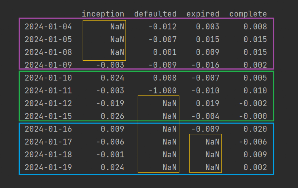
Let’s create price data for four hypothetical assets over 13 days:

• inception: Asset with a later inception date.

• defaulted: Asset that defaulted.

• expired: Asset that expired.

• complete: Asset with a complete price history.

We’ll convert these prices to returns and split the dataset into 3 rebalancing periods of 4 days each.

import datetime as dt

import matplotlib.image as mpi
import matplotlib.pyplot as plt
import numpy as np
import pandas as pd
from sklearn import set_config
from sklearn.impute import SimpleImputer
from sklearn.model_selection import GridSearchCV
from sklearn.pipeline import Pipeline

from skfolio.model_selection import WalkForward, cross_val_predict
from skfolio.optimization import EqualWeighted
from skfolio.pre_selection import SelectComplete, SelectNonExpiring
from skfolio.preprocessing import prices_to_returns


def generate_prices(n: int) -> list[float]:
    # Just for example purposes
    return list(100 * np.cumprod(1 + np.random.normal(0, 0.01, n)))


prices = pd.DataFrame(
    {
        "inception": [np.nan] * 3 + generate_prices(10),
        "defaulted": generate_prices(6) + [0.0] + [np.nan] * 6,
        "expired": generate_prices(10) + [np.nan] * 3,
        "complete": generate_prices(13),
    },
    index=pd.date_range(start="2024-01-03", end="2024-01-19", freq="B"),
)

X = prices_to_returns(prices, drop_inceptions_nan=False, fill_nan=False)

img = mpi.imread("../images/incomplete_dataset.png")
fig, ax = plt.subplots(figsize=(10, 6.327))
ax.imshow(img)
ax.axis("off")
plt.subplots_adjust(left=0, right=1, top=1, bottom=0)

Pipeline

Our Pipeline will handle the following cases:

When we train our optimization model on the first period (magenta box), we want to exclude the “inception” asset.

When testing on the second period (green box), we want to capture the loss on the “defaulted” asset (the -100% on 2024-01-11) without failing on the subsequent NaNs.

Then, when we train on the second period, we want to include the “inception” asset, exclude the defaulted asset, and also exclude the “expired” asset that will expire in the next test period (blue box).

set_config(transform_output="pandas")

model = Pipeline(
    [
        ("select_complete_assets", SelectComplete()),
        (
            "select_non_expiring_assets",
            SelectNonExpiring(
                expiration_dates={"expired": dt.datetime(2024, 1, 16)},
                expiration_lookahead=pd.offsets.BusinessDay(4),
            ),
        ),
        ("zero_imputation", SimpleImputer(strategy="constant", fill_value=0)),
        ("optimization", EqualWeighted()),
    ]
)

The transformer SelectComplete handles the “inception” and “defaulted” assets, while SelectNonExpiring excludes assets close to expiration. SimpleImputer replaces NaNs with 0s on the “defaulted” asset in the test period.

Walk-Forward Cross-Validation

Now, we pass this pipeline model into cross_val_predict using WalkForward:

pred = cross_val_predict(model, X, cv=WalkForward(train_size=4, test_size=4))

As expected, the pipeline correctly applies our rules to each period:

df = pred.composition
df.columns = ["Period 2 (green)", "Period 3 (blue)"]
df

	Period 2 (green)	Period 3 (blue)
asset
defaulted	0.333333	0.0
expired	0.333333	0.0
complete	0.333333	0.5
inception	0.000000	0.5

And from the out-of-sample returns, we can see that the default event was captured on 2024-01-11:

df = pred.returns_df
df

2024-01-10    0.000883
2024-01-11   -0.319223
2024-01-12    0.002128
2024-01-15   -0.005024
2024-01-16   -0.007138
2024-01-17    0.000097
2024-01-18   -0.002757
2024-01-19   -0.003622
Name: returns, dtype: float64

Step-by-Step Fitting with WalkForward

Let’s break down the cross_val_predict by calling fit and predict on each period:

print("Rebalancing Period 1")
model.fit(X.iloc[:4])
portfolio = model.predict(X.iloc[4:8])
print(portfolio.composition)
print(portfolio.returns)

print("Rebalancing Period 2")
model.fit(X.iloc[4:8])
portfolio = model.predict(X.iloc[8:])
print(portfolio.composition)
print(portfolio.returns)

Rebalancing Period 1
           EqualWeighted
asset
defaulted       0.333333
expired         0.333333
complete        0.333333
[ 0.00088251 -0.31922336  0.00212848 -0.00502352]
Rebalancing Period 2
           EqualWeighted
asset
inception            0.5
complete             0.5
[-7.13803938e-03  9.68108599e-05 -2.75703615e-03 -3.62232125e-03]

Hyper-Parameter Tuning

The Pipeline model can also be passed to GridSearchCV to find the optimal hyperparameters for a specified score (by default, the out-of-sample average Sharpe ratio). For example, we could use it to find the optimal exit time before a bond expires:

grid_search = GridSearchCV(
    estimator=model,
    cv=WalkForward(train_size=4, test_size=4),
    param_grid={
        "select_non_expiring_assets__expiration_lookahead": [
            pd.offsets.BusinessDay(i) for i in range(20)
        ],
    },
)
grid_search.fit(X)
model = grid_search.best_estimator_