Backtesting and Evaluation#

In skfolio, portfolio construction methods produce target weights that specify the allocation selected at each rebalancing date. Evaluating these allocations over subsequent observations involves two separate modelling choices:

whether to compute portfolio returns at fixed target weights throughout each holding period or at weights that evolve with asset returns between rebalances
whether to sum the resulting portfolio returns arithmetically or compound them into a wealth index

The choice of weights determines the portfolio return series, while the accumulation method determines cumulative returns and drawdown measures. The same target allocations can therefore produce different performance statistics under these conventions. The appropriate settings depend on the evaluation objective:

Allocation skill (ex-ante). Estimate the expected return and risk attributable to the target allocations selected by the portfolio construction process. The aim is to evaluate the allocation decisions themselves, independently of subsequent changes in weights caused by relative asset returns.
Expected performance of the implemented strategy. Estimate the expected return and risk of rebalancing to the target weights at scheduled dates and allowing the resulting holdings to evolve with asset returns between those rebalances. Turnover and transaction costs are computed relative to the previous period’s ending weights, including drift, rather than its target weights.
Relative strategy performance. Estimate the difference in expected performance between portfolio strategies. The appropriate implementation convention depends on whether the comparison concerns the target allocation decisions or the strategies as they would be implemented between rebalances. When strategies are evaluated on the same out-of-sample dates, common biases may cancel and positively correlated sampling errors can reduce the uncertainty of the difference.
Historical realization (ex-post). Reconstruct the holdings, trades, wealth and drawdowns that would have occurred along the observed return path under the stated implementation assumptions.

The first three objectives involve estimating expected performance from out-of-sample returns. The observed history is one finite realization of the process generating returns, so these estimates may be biased and are subject to sampling uncertainty.

In an ex-post evaluation, holdings, trades, wealth and drawdowns are reconstructed along the observed return path under the stated implementation assumptions. A more accurate reconstruction does not necessarily improve estimates of expected performance on another sample of returns.

In skfolio two parameters control these modelling choices:

weight_drift determines the weights used to compute each observation’s return. With False, returns are computed at the target weights (no drift), which remain constant within each holding period. With True, each holding period starts at the target weights, but the weights used for subsequent observations evolve with asset returns until the next scheduled rebalance. Returns are therefore computed from drifted weights.
compounded determines how the resulting portfolio returns are accumulated. With False, cumulative returns are an arithmetic sum. With True, they form a compounded wealth index. This setting affects drawdown measures, but leaves the underlying return series unchanged.

Both default to False. The default therefore evaluates allocation skill (ex-ante) at target weights, consistent with the optimizer’s linear portfolio return definition, and accumulates returns arithmetically.

Choosing the settings#

weight_drift and compounded are independent, and all four combinations are valid. The table gives suggested settings for each evaluation objective.

Suggested starting points#
Objective	`weight_drift`	`compounded`
Allocation skill (ex-ante), before transaction costs	`False`: target weights (no drift)	`False`
Expected performance of the implemented strategy	`True`: drifted weights	`False`
Relative strategy performance	`False`: target weights (no drift). `True`: drifted weights.	`False`
Historical realization (ex-post): wealth and percentage drawdowns	`True`: drifted weights	`True`

compounded changes cumulative returns, drawdown measures and ratios based on drawdowns. Measures computed from individual returns, such as mean return, variance, VaR, CVaR, and the Sharpe and Sortino ratios, are unchanged, as are their sampling variances.

weight_drift changes the underlying returns and can change both the bias and sampling variance of performance estimates for the chosen evaluation objective.

Reconstructing holdings and trades more accurately does not necessarily improve estimates of expected performance. An evaluation at target weights can have lower mean squared error if its reduction in sampling variance outweighs its squared bias. See Estimating expected return.

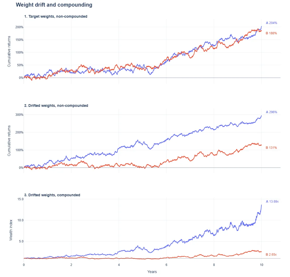
The figure below compares the effects of weight drift and compounding on two illustrative ten-year paths from the same asset return model. The simulations use equal target weights and annual rebalancing, with identical target allocations across settings. The paths were selected to illustrate the differences. The observed gaps do not estimate the typical effect of drift or compounding.

Two simulated portfolio paths evaluated with target weights, drifted weights, and drifted weights with compounding

How weight drift changes returns#

Let \(r_t\) be the vector of asset returns during observation \(t\), and \(w_k\) the target weights set at rebalancing date \(t_k\). The holding period runs from \(t_k\) to just before \(t_{k+1}\). The equations in this section describe returns before transaction costs and fees.

Target weights (no drift)#

With weight_drift=False, every observation within the holding period uses the same target weights:

\[r^{target}_t = w_k \cdot r_t, \qquad t_k \le t < t_{k+1}.\]

It is consistent with the optimizer’s linear portfolio definition and is the default convention for evaluating allocation skill: the expected return and risk of the target allocations are assessed independently of subsequent holdings drift. Economically, it is equivalent to restoring the target weights after every observation without charging for those within-period trades.

Drifted weights#

With weight_drift=True, let \(u_t\) be the weights held at the start of observation \(t\). Each position grows with its asset’s return:

\[r^{drifted}_t = u_t \cdot r_t, \qquad u_{t+1} = \frac{u_t \circ (1 + r_t)}{1 + u_t \cdot r_t}, \qquad u_{t_k} = w_k,\]

where \(\circ\) denotes element-wise multiplication. The weights reset to the next targets at \(t_{k+1}\).

For example, starting with 50% in each of two assets, if the first asset gains 10% and the second is unchanged, the portfolio gains 5%. The next observation then starts with weights of 52.38% and 47.62% under weight_drift=True, whereas an evaluation at target weights continues to use 50% and 50% again.

If the first asset outperforms again, the portfolio with holdings drift has a higher return than the target-weight portfolio because it now has greater exposure to that asset. If relative performance reverses, it has a lower return. Momentum and reversal can therefore affect the performance of the strategy under the two modelling conventions.

The drift equation is self-financing, with changes in weights arising from asset returns rather than from external cash entering the portfolio. A portfolio that is rebalanced to its target weights can also be self-financing, since purchases can be funded by sales of other assets. The conventions differ in whether target weights are restored within the holding period.

Portfolio raises an error when wealth becomes non-positive because the weights for the next observation are then undefined. This can occur, for example, in leveraged or short portfolios following sufficiently large adverse returns.

Turnover and transaction costs#

At each scheduled rebalancing, turnover is computed from the difference between the new target weights and either the previous target weights or the drifted ending weights, depending on the evaluation convention.

Let \(\tilde w_k\) denote the weights held at the end of holding period \(k\). The two conventions give

\[\text{target turnover} = \|w_{k+1}-w_k\|_1, \qquad \text{executed turnover} = \|w_{k+1}-\tilde w_k\|_1.\]

With weight_drift=False, previous_weights contains the previous portfolio’s target weights. Target turnover measures the change between successive target allocations.

With weight_drift=True, previous_weights contains the weights held at the end of the previous holding period. Executed turnover measures the trades required to move from these holdings to the new target allocation.

Drift reduces turnover when relative asset returns move the existing holdings toward the next target and increases it when they move the holdings away from that target. This can reduce trading for momentum strategies and increase it for reversal strategies.

For any given pair of targets, the triangle inequality gives

\[|\text{executed turnover} - \text{target turnover}| \le \|\tilde w_k-w_k\|_1.\]

With a sequential splitter, cross_val_predict passes each successful portfolio’s ending_weights as previous_weights to the next fit when previous holdings are needed. With drift disabled, ending_weights contains the target weights. With drift enabled, it contains the weights held at the end of the period. Transaction costs and turnover constraints are computed from these previous weights. Enabling drift therefore makes the folds run sequentially and propagates ending weights even without costs or a turnover constraint. When fits are independent, previous weights are assigned to the predicted portfolios afterward for turnover and cost calculations.

When asset selection changes between rebalances, turnover and transaction costs are calculated assuming full liquidation of positions in assets absent from the new universe. In a pipeline, set_output(transform="pandas") preserves the asset names needed to match previous holdings to the new selection. For assets absent from X, transaction_costs must be a single rate applied to all assets or a dictionary keyed by asset name.

For a direct predict call, transaction costs use the supplied previous_weights under either drift setting.

The following example rebalances every five observations, applies a one-off cost rate of 10 basis points on traded notional, and limits turnover in each asset to 30% of portfolio value at each rebalance:

from skfolio.optimization import MeanRisk

holding_period = 5
tc_rate = 0.001
model = MeanRisk(
    transaction_costs=tc_rate / holding_period,
    max_turnover=0.3,
)
pred = cross_val_predict(
    model,
    X,
    cv=WalkForward(train_size=252, test_size=holding_period),
    portfolio_params={"weight_drift": True, "compounded": False},
    entry_rebalancing_params={"max_turnover": None},
)

max_turnover=0.3 is a per-asset constraint. Total portfolio turnover can exceed 30%. entry_rebalancing_params removes this constraint for the initial trade from cash. The constraint applies from the second rebalance onward. This limit does not apply to the assumed liquidation of positions outside the investment universe.

With transaction costs or turnover constraints, the next target allocation can also differ depending on whether the optimization uses the previous target weights or the portfolio weights at the end of the holding period. Evaluating the same sequence of targets under both settings isolates the effect of holdings drift on returns and turnover.

Transaction cost convention#

The optimizer expresses expected returns per observation, while transaction costs are paid once when a rebalance occurs. To express the two quantities on the same basis, a one-off transaction cost is divided by the expected holding period to obtain a cost per observation. Portfolio evaluation uses the same convention. See periodicity convention for the rationale and conversion examples.

For a one-off transaction cost rate \(c\) and an intended holding period of \(n\) observations, set transaction_costs to \(c/n\), as in the example above.

If turnover is \(q_k\), each observation in that period is reduced by \(cq_k/n\). Over exactly \(n\) observations, these deductions sum to \(cq_k\) in arithmetic-return units.

Charging the full transaction cost on the trade date would produce a different observation-level return series and, after compounding, a different wealth path. It would also change tail-risk and drawdown measures.

Both weight conventions use the same transaction-cost convention. If the actual holding period contains \(m\) observations, a fixed input \(c/n\) deducts a total of \(mcq_k/n\) in arithmetic-return units. This matters for calendar-based rebalancing and incomplete periods, where the number of observations varies.

ending_weights are the portfolio weights at the end of the holding period. With weight_drift=False, they equal the target weights. With weight_drift=True, they reflect the effect of asset returns through the final observation. They are calculated before transaction costs and management fees because those costs reduce reported portfolio returns but are not deducted from a modelled cash balance or individual position.

Management fees remain based on the target weights selected for the holding period rather than on subsequent changes in weights caused by asset returns.

Return aggregation and compounding#

For a given portfolio return series \(r^{ptf}_t\), arithmetic accumulation is

\[A_T = \sum_{t=1}^T r^{ptf}_t.\]

Compounding produces a wealth index, expressed per unit of starting capital:

\[W_T = \prod_{t=1}^T(1+r^{ptf}_t).\]

skfolio reports the compounded series as this wealth index. Its total return is \(W_T-1\).

Use compounded=True for measures based on compounded wealth, including compounded total return and percentage drawdown. This applies to both out-of-sample estimation and historical reconstruction.

Changing compounded does not change the optimizer’s objective or the underlying observation-level portfolio returns.

See Data Preparation for the discussion of simple and logarithmic returns.

For fixed targets within one holding period, before costs and fees, compounding gives

\[W^{target} = \prod_t(1+w_k\cdot r_t), \qquad W^{drifted} = \sum_i w_{k,i}\prod_t(1+r_{i,t}) + 1-\sum_i w_{k,i}.\]

The first expression describes restoring the target weights after every observation. The second describes implementing the target allocation and holding the resulting positions until the next scheduled rebalance. The final term is the implicit zero-return cash position when the explicit asset weights do not sum to one.

Changing the order of asset returns within this holding period leaves both terminal wealth values unchanged, provided wealth stays positive. At target weights, it also leaves mean return and variance unchanged. With holdings drift, the portfolio return series can change because holdings depend on earlier returns. Intermediate wealth and drawdowns depend on return order in both settings.

Configuring an evaluation#

For a direct call to an optimizer’s predict, set the options in the optimizer’s portfolio_params. For cross_val_predict and online_predict, pass them in the function’s portfolio_params.

The following example applies three combinations of the settings to the same historical data, with rebalancing every 21 observations. X contains asset returns in decimal form, ordered by date, with one column per asset.

from skfolio.datasets import load_sp500_dataset
from skfolio.model_selection import WalkForward, cross_val_predict
from skfolio.optimization import EqualWeighted
from skfolio.preprocessing import prices_to_returns

prices = load_sp500_dataset()
X = prices_to_returns(prices)

model = EqualWeighted()
cv = WalkForward(train_size=252, test_size=21)

target_evaluation = cross_val_predict(model, X, cv=cv)

drifted = cross_val_predict(
    model, X, cv=cv, portfolio_params={"weight_drift": True, "compounded": False}
)

compounded_wealth = cross_val_predict(
    model, X, cv=cv, portfolio_params={"weight_drift": True, "compounded": True}
)

target_evaluation evaluates the target weights and accumulates the resulting returns arithmetically. drifted starts each holding period at the same target weights but allows the holdings to evolve with asset returns until the next rebalance. Its returns are also accumulated arithmetically. compounded_wealth uses the same holdings-based return construction as drifted and compounds those returns into a wealth index.

The example illustrates the settings on historical data. It does not reproduce the simulated figure. With daily equity data, 21 observations approximate a month. Use calendar-based splits when rebalancing must occur on specific dates.

Each walk-forward call returns a MultiPeriodPortfolio containing one Portfolio per test period. weight_drift applies to each child portfolio. compounded applies to both the children and the resulting MultiPeriodPortfolio. Function-level values override the optimizer’s portfolio_params. Omitted values are inherited. See Cross-Validation Prediction for the complete routing rules.

compounded can also be changed after construction. To compound the existing drifted return series without repeating the evaluation, use:

drifted.compounded = True
drifted.plot_cumulative_returns()

This changes the aggregate object’s cumulative returns and drawdown measures. Each child portfolio has its own compounded setting. weight_drift is fixed at construction because changing it would change the portfolio return series.

Holding periods and validation#

A direct predict(X) call treats all of X as one holding period. With drift enabled, the portfolio starts at its target weights and positions are held throughout that window. In a walk-forward evaluation, each test period starts at its predicted target weights. The length of the test period therefore sets the interval between scheduled rebalances.

Different validation schemes can represent different types of evaluation path:

WalkForward produces one sequential path.
online_predict builds a path from a single stateful estimator updated with partial_fit. See Online Learning.
MultipleRandomizedCV runs walk-forward evaluations on randomly selected asset subsets and, optionally, contiguous time windows.
CombinatorialPurgedCV evaluates combinations of test blocks and can train on observations later than a given test block. Its reconstructed paths therefore do not represent strictly forward historical simulations.

See Cross-Validation Prediction for purging, embargoing and supported splitters.

Estimating expected return#

The sample means of the portfolio returns, computed with and without weight drift, are two estimators of expected return. For the same target allocations, the bias introduced by the choice of weights depends on the evaluation objective.

Before transaction costs, the return contribution from drift at observation \(t\) is

\[d_t = r^{drifted}_t-r^{target}_t = (u_t-w_k)\cdot r_t.\]

Its expected contribution to the sample mean over \(T\) observations is \(\bar d = \frac{1}{T}\sum_{t=1}^T\mathbb{E}[d_t]\). The expected transaction cost difference per observation, \(b\), is the expected cost of executed turnover minus the expected cost of target turnover.

Allocation skill (ex-ante). Before transaction costs, weight_drift=False evaluates the target allocations directly and introduces no bias from subsequent holdings drift. weight_drift=True introduces drift contribution \(\bar d\).
Expected performance of the implemented strategy. For expected net return, weight_drift=True includes both holdings drift and the transaction costs associated with executed turnover. weight_drift=False introduces bias \(b-\bar d\).

The expected gross-return difference between the two settings can be negligible with frequent rebalancing. In two illustrative simulations, it is about 0.2 bp p.a. for a diversified 50-asset portfolio rebalanced weekly and about 2% p.a. for a concentrated four-asset high-volatility portfolio rebalanced quarterly.

These are stylized simulations, not empirical estimates for particular asset classes. They use equal target weights and geometric Brownian asset prices. The calculation appendix gives the assumptions and formulas.

The sample means also vary from one sample to another. Their sampling variances measure this variability. In the same examples, drift increases the sampling variance of the estimated gross mean by less than 0.01% for the diversified portfolio and about 3% for the concentrated high-volatility portfolio. Serial correlation also affects sampling variance. A long-run variance estimate [1] accounts for dependence between observations.

Mean squared error (MSE) combines squared bias with sampling variance. \(V_{\mathrm{target}}\) and \(V_{\mathrm{drifted}}\) denote the sampling variances of the two estimated net means. When the drifted mean is unbiased for the implemented strategy’s expected net return under the return model, the MSEs are

\[\operatorname{MSE}_{\mathrm{target}}=(b-\bar d)^2+V_{\mathrm{target}}, \qquad \operatorname{MSE}_{\mathrm{drifted}}=V_{\mathrm{drifted}}.\]

The estimate at target weights has lower MSE when its reduction in sampling variance exceeds its squared bias. Including holdings drift can also reduce sampling variance, in which case the drifted estimate has lower MSE.

For the concentrated high-volatility example, a portfolio volatility of 66% p.a. gives a standard error of about 30% for the annualized target-weight mean over five years (\(66\%/\sqrt{5}\)). When estimating the implemented strategy’s expected gross return, its squared bias is only about 0.45% of its sampling variance. Its MSE is therefore close to that of the drifted estimate. With longer samples, sampling variance decreases while a persistent bias remains.

Appendix: Calculation details#

The illustrative examples assume \(N\) equally weighted assets, rebalanced every \(n\) observations, with \(A\) observations p.a. Asset prices follow geometric Brownian motions with equal exposure to a common market factor and independent asset-specific shocks. Returns are independent across observations, and transaction costs are excluded.

Let \(\sigma_p\) be the annual portfolio volatility at target weights, \(\sigma_\epsilon\) the annual asset-specific volatility, and \(s\) the standard deviation of annualized expected arithmetic asset returns. With \(h=(n-1)/A\), the annualized expected gross drift contribution \(\bar d_{\mathrm{ann}}\) and relative change in sampling variance \(\gamma\) are, to leading order,

\[\bar d_{\mathrm{ann}} \approx \frac{h s^2}{2}, \qquad \gamma \approx \frac{h(N-1)\sigma_\epsilon^4}{2N^2\sigma_p^2}.\]

The variance change \(\gamma\) is measured relative to the sampling variance of the estimated gross mean at target weights.

Diversified weekly-rebalancing example. \(N=50\), \(n=5\), \(A=252\), \(\sigma_p=15\%\), \(\sigma_\epsilon=21\%\) and \(s=5\%\).
Concentrated high-volatility quarterly-rebalancing example. \(N=4\), \(n=91\), \(A=365\), \(\sigma_p=66\%\), \(\sigma_\epsilon=87\%\) and \(s=40\%\).

References